Statistical interpretation of the daily variation of urban water consumption in Beijing, China

Abstract

The efficient planning and design of water networks, as well as the management and strategies of existing water supply systems, require accurate short-term water demand forecasts. In this study, a statistical model for the estimation of daily urban water consumption was developed. The model was applied to analyse and forecast the daily water consumption in the main district of Beijing, China, from 2006 to 2010. The model exhibited good performance with a coefficient of determination, R², greater than 0.9 in both the calibration and validation periods. The results indicate that: (a) the 7-day moving average temperature is an efficient variable that can be used to depict water-use variation in a year; (b) a daily maximum temperature of 31.1°C and the occurrence of precipitation are two thresholds of water-use behaviour; and (c) the current day’s water consumption has a strong correlation with the consumption of one, two and seven days ago.

Editor Z.W. Kundzewicz; Associate editor D. Yang

Citation Zhang, D.W., et al., 2013. Statistical interpretation of the daily variation of urban water consumption in Beijing, China. Hydrological Sciences Journal, 59 (1), 181–192.

Résumé

La planification efficace et la conception des réseaux d’eau, ainsi que la gestion et les stratégies des systémes d’approvisionnement en eau existants, nécessitent des prévisions de la demande en eau précises à court terme. Dans cette étude, un modéle statistique pour l’estimation de la consommation d’eau quotidienne urbaine a été élaboré. Le modéle a été appliqué pour analyser et prévoir la consommation d’eau quotidienne dans le quartier principal de Beijing en Chine, de 2006 à 2010. Le modéle présente de bonnes performances avec un coefficient de détermination R² supérieur à 0,9 à la fois pour les périodes d’étalonnage et de validation. Les résultats indiquent que (a) la moyenne mobile à 7 jours de la température est une variable efficace qui peut ètre utilisée pour représenter la variation de l’utilisation de l’eau sur une année; (b) une température maximale quotidienne de 31,1°C et la survenue de précipitations sont deux seuils de comportement de l’utilisation de l’eau, et (c) la consommation d’eau du jour courant a une forte corrélation avec la consommation d’eau, un, deux et sept jours plus tôt.

Key words:

• daily urban water consumption
• time series analysis
• statistical regression
• threshold model
• Beijing, China

Mots clefs:

• consommation quotidienne de l’eau urbaine
• analyse des séries chronologiques
• régression statistique
• modéle de seuil
• Beijing, Chine

INTRODUCTION

Nowadays, urban population has outnumbered rural population. The world has 26 metropolitan areas, each with more than 10 million inhabitants. Nearly 500 conurbations surround these metropolitan areas, each with a population in excess of 1 million (Kowalczak and Kundzewicz 2011). The continuous growth of population and urbanization is expected to result in a significant increase in water demand in the first half of the 21st century (Richard and Parker 2009). Efficiently managing water resources in a highly urbanized region has become imperative. Analysing daily urban water consumption and forecasting future demand tendency have become essential for the advanced planning, design, operation and management of water networks.

In China, since the reform and open-up policy of the late 1970s, the country has undergone an era of rapid urbanization. At the end of 2009, the urban population in China comprised over 620 million, with an urbanization rate of 46.4%. This rate is forecast to reach 60% in 2015 (CASS 2010). Nearly 400 of the 669 medium to large cities in China are facing water scarcity; even worse, 110 cities are in a severe situation. Urban water shortage results in an annual economic loss of more than 200 billion RMB and affects approximately 40 million people.

As the capital city of China, Beijing is undergoing a rapid socio-economic development and a population explosion. Water resources per capita, including both groundwater and surface water, were only approx. 100 m³ for the year 2009. Moreover, the groundwater level is lowering at a speed of 1.1 m per year because of continuous over-abstraction (Beijing Water Authority 2009). Water availability has become a bottleneck to economic development, as well as a focus in ecological environment improvement. A single-resource supply system is no longer sufficient for Beijing’s water supply. A system of multiple water sources, that are surface water, groundwater, reclaimed water and diverted water, has become the main trend. Furthermore, the efficient operation and management of such a complex water supply system requires accurate short-term urban water-use forecasting, which, to our knowledge, has not yet been carefully studied in Beijing.

Characterized by complex interactions between human and natural variables at multiple spatial and temporal scales, urban water use reflects a coupled human and natural system (House-Peters and Chang 2011). The strength of the feedback and implications of nonlinear responses have not been fully revealed because of the complexity of such responses. Water demand forecasting can generally be classified into two types: short term and long term. Short-term water demand forecasting refers to daily, weekly or monthly forecasting, whereas long-term forecasting means annual forecasting or longer. Insufficient data and complicated mechanisms cause most studies to focus on urban water consumption based on annual or monthly data, with only a few dealing with daily water consumption.

Maidment et al. (1985) developed a short-term forecasting model for Austin, Texas, USA, based on the Box–Jenkins time series analysis using daily data on water use and the corresponding weather. Maidment and Miaou (1986) applied the model to nine American cities located in Florida, Pennsylvania and Texas for the same analysis period. They concluded that a nonlinear relationship exists between water consumption and temperature. Moreover, the model performance is limited by the endogenous randomness of the water consumption in small cities.

Zhou et al. (2000) also conducted a time series analysis for Melbourne, Australia. In their analysis, daily water consumption is considered as the sum of trend and seasonal use, with the latter being further divided into seasonal, climatic and persistent components. Evaporation, antecedent precipitation index and some other climatic factors were employed as regression variables. The model yielded a coefficient of determination, R², value of 90% in a test run using a cross-validation procedure and an independent data set for the summer period from 1 December 1996 to 31 January 1997.

Bougadis et al. (2005) compared short-term water consumption forecasting models using regression, time series analysis and artificial neural network techniques. The models were run on data from the city of Ottawa, Ontario, Canada, with the conclusion that current and future water use are highly correlated with daily precipitation, maximum temperature and historical water consumption.

Gato et al. (2007) studied the daily urban water demand of East Doncaster, Victoria, Australia, indicating that base consumption can be rather weather insensitive. They also suggested that the day of the week affects base consumption and that seasonal water use is reduced due to precipitation.

Wong et al. (2010) analysed the daily water consumption of Hong Kong from 1 December 1990 to 31 January 2007. In the study, the holiday effect was introduced, including that of Chinese traditional holidays, and the contribution of each factor to the water consumption was analysed. The model performed well with a R² value of 76%.

In the aforementioned studies, urban water use is divided into base and seasonal components, and different mathematical formulations are proposed by employing various climate and holiday factors, among others. However, the focus of these studies is limited to cities with a relatively stable condition in developed countries. Whether this statistical framework can be introduced to interpret the daily variation in urban water consumption in Beijing, a rapidly developing metropolitan area, remains unknown. Meanwhile, different components of urban water consumption in Beijing call for more precise descriptions. Moreover, the factors that are most relevant to these components and unique to Beijing should be discovered to aid more efficient urban water-use forecasting and management.

This article aims to develop a statistical model of daily water use in the main district of Beijing. The model has the potential to: (a) study the inter-annual trend of Beijing water use as a result of socio-economic development; (b) investigate daily water-use pattern response to climate variation; (c) confirm the effect of the day of the week on water-use persistence, and (d) forecast future water use in Beijing. The findings of this study may improve the understanding of daily urban water consumption and contribute to the efficient operation of the urban water supply system in Beijing.

STUDY AREA AND DATA

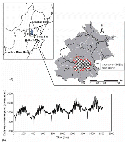
Located in the northwest of the North China Plain, Beijing, covers an area of 16 808 km², 62% of which is mountainous. Beijing has a semi-arid and semi-humid continental monsoon climate. The annual average temperature is 14.0°C, ranging from –4°C in January to 26°C in July. Annual precipitation is approximately 595 mm and is unevenly distributed, with about 80% occurring between June and August.

In 2009, the total water consumption of Beijing was 3.55 billion m³; the shares of the domestic, industrial, agricultural and environmental sectors accounted for 41, 15, 34 and 10%, respectively. In terms of water sources, reservoirs contributed 13%, groundwater 62%, reclaimed water 18% and water diverted from outside the city 7% (Beijing Water Authority 2009). Given that both the amount and the quality of water vary with different sources, accurate forecasting of water demand is necessary for the efficient and safe operation and management of the water supply system.

Beijing water supply region can be divided into the central urban and sub-urban areas. Established in 1999, Beijing Waterworks Group provides residential water for the six urban districts of Beijing, which cover a residential area of 1373 km². Only monthly water consumption data are available for the period 1999–2005. Daily water consumption data (m³ d^-1) from the Group is used in this study. The data set covers the period from 1 January 2006 to 31 December 2010, as shown in Fig. 1. A complete daily data set is available only for this period. The corresponding climate data sets, which include air temperature (°C), wind speed (m s^-1) and precipitation (mm), were obtained from the Beijing Climate Observatory, a national station with number 54 511. Moreover, holiday information for each day was collected. The data set for the first four years, that is 2006–2009, was used for model calibration, whereas the data set for the last year, 2010, was employed for model validation.

Fig. 1 (a) Location of the study area, Beijing main district and (b) daily urban water consumption in Beijing from 2006 to 2010.

METHODOLOGY

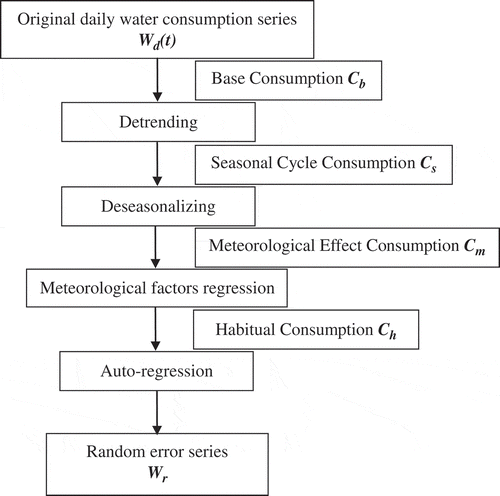
In this study, statistical techniques based on time series analysis were adopted to identify the characteristics of urban water consumption. Daily water consumption is decomposed into the base, seasonal and habitual components, which are mainly affected by long-term, annual and daily factors, respectively, as shown schematically in Fig. 2. Daily water consumption is expressed as follows:

(1)

Fig. 2 Daily water consumption analysis model of Beijing main district.

where W_d(t) is the daily water consumption series and is the random error series expected to exhibit normal distribution after transformation. The first three items on the right-hand side of equation (1), namely, base, seasonal cycle and habitual consumption, can be treated as inter-annual, inner-annual and weekly time scales, respectively.

To simplify the analysis, we assume that these three parts of water consumption are independent of one another and are linearly additive, although they may have a certain intrinsic correlation and may be a nonlinear system in actual situations.

Base component

The base component reflects the long-term water-use trend of a city, which fluctuates with the synthesized effects of socio-economic factors, such as population, household income and gross domestic product (GDP), as well as water price and other policy restrictions. Efforts have been made to find a robust response function of water consumption to these factors at different time scales, but to date it remains a challenging task (Brookshire et al. 2002, Dalhuisen et al. 2003, Arbues and Villanua 2006, Worthington and Hoffman 2008). In this study, we assume the minimum daily water consumption in each year, mainly occurring in winter, as the base consumption and obtain the trend by regressing directly against the time in days when the lowest water use occurs. Considering that the registered floating population accounts for 40% of the total population in Beijing (CASS 2011), instead of daily per capita consumption, total daily water consumption is adopted to represent the base consumption. The base component can be formulated as:

(2)

where C_b(d) denotes base water use; hereinafter, a caret (^) indicates estimated values; n is the order of the polynomial function; β₀, β₁, β₂, …, β_n, are the coefficients; d is the time (in days) and d = 1 corresponds to the first daily observation.

Seasonal component

The seasonal component is the part of urban water use that mainly varies in a seasonal pattern and weather conditions over the past few days. Therefore, the seasonal component, S_d, is further divided into two parts: , which changes according to the seasonal weather fluctuation pattern, and , which changes based on the recent daily weather conditions. These two parts make up seasonal consumption, which is expressed as:

(3)

Seasonal cycle

Average air temperature is usually taken as a representative variable of seasonal weather variation. Various methods can be adopted to characterize seasonal water consumption variation:

1. a heat function that is a linear regression of against a seasonal cycle factor, such as average temperature;

2. an auto-regressive model of with coefficients reflecting seasonality;

3. a discrete Fourier transformation (DFT) of .

Of these methods, the DFT is simple and performs well. Thus, DFT is widely used. However, DFT is only a mathematical transformation, and so the Fourier series do not reflect the physical mechanism in an explicit manner, and the effect of average temperature variation on seasonal water consumption cannot be revealed under extreme climate conditions. In this study, referring to the evident weekly water-use pattern, we employ the 7-day moving average temperature as an independent variable to describe the seasonal consumption variation, as follows:

(4)

where represents the 7-day moving average temperature for the most recent seven days.

Daily meteorological effect

Daily urban water consumption is sensitive to temperature and precipitation (Miaou 1990, Protopapas et al. 2000, Schleich and Hillenbrand 2009) in terms of maximum temperature, amount and duration of precipitation, and so on. In this study, the threshold model (Tong 1983) is employed to determine the relationships between daily water consumption and weather variables such as maximum temperature, maximum wind speed, precipitation amount and duration. Weather data of the present day and of the past few days are considered to allow us to identify the principal factors and determine the related threshold values. The threshold model adopted is as follows:

(5)

where x_i represents different kinds of weather data, and b is the threshold value of the most significant variable.

Habitual component

Water use is a process affected not only by physical, but also by habitual factors. For instance, most families prefer to conduct house cleaning and clothes washing on weekends. Habitual consumption reflects the water-use habit, which is characterized by external randomness but inner regularity. The habitual component is expressed by an auto-regression model:

(6)

where refers to habitual consumption; p is the order of the autoregressive procedure, AR(p); and φ₀, φ₁, φ₂, …, φ_p are the coefficients of AR(p).

Model performance

The performance of a mathematical model can be quantified by using many standard statistical parameters that describe the errors associated with the model forecasts. As an indication of the fitting result between observed and predicted values, the coefficient of determination (R²), the average absolute relative error (AARE) and the threshold statistic for a level of x% (TS_x) were calculated.

The coefficient of determination, R², is defined by:

(7)

where is the sum of square deviations from the mean value, called initial variance; is the mean of actual consumption; is the sum of square deviations from the estimated value, called residential variance, and is simulated water consumption. When the value of R² is close to unity, the model can perfectly reproduce the recorded consumption.

The AARE is a quantitative measure of the average error. A smaller value of AARE denotes better performance of the model; it is expressed as follows:

(8)

Finally, TS_x is a measure of the consistency of forecasting errors of a model and can be computed as:

(9)

where Y_x is the number of data points with an absolute relative error less than x% from the model, and N is the number of total data samples. A larger TS_x evidently indicates better performance of the model. The threshold statistics are calculated for several levels of absolute relative errors: 1, 3, 5, 10 and 15%.

RESULTS

Base component

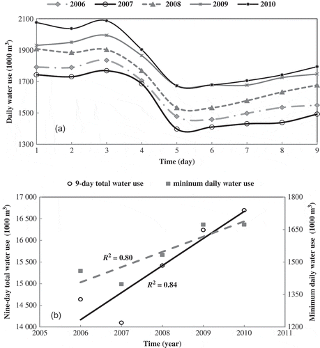
The day of the year with the minimum water consumption always falls on the Lunar New Year’s Eve, the most important day of the traditional Chinese Spring Festival holiday. During the associated holiday period, water consumption is remarkably lower than usual, and this variation pattern is identical every year (Fig. 3(a)). Given that a large population of non-local people working in Beijing go back to their hometowns and local people make excursions out of town during the Chinese Spring Festival, a significant decrease in water consumption is observed. In addition, other holidays such as National Day and Labour Day may have a similar effect on related water consumption, but are not considered in this article. Figure 3(b) shows that the daily minimum water use and the 9-day total consumption both increased linearly over the recent 5 years.

Fig. 3 (a) Daily water-use variation during the excluded 9-day period associated with the Chinese Spring Festival, 2006–2010 (the fifth day is the Lunar New Year’s Eve) and (b) linear increase in 9-day total water use and minimum daily water use.

To avoid the significant effect of Chinese traditional holidays, data on the nine days around the Lunar New Year’s Eve were excluded and the minimum daily water consumption selected as the base use from the remaining time series. The base consumption of Beijing in recent years shows an evident increasing trend, and a linear equation is obtained as:

(10)

where is the estimated daily base water use (in m³ d^-1), d = 1, 2, 3, … and d = 1 corresponds to 1 January 2006, which is the first daily observation of water use.

From 2006 to 2009, base consumption increased at a rate of approximately 280 m³ d^-1 because of the synthesized effects of population increase, socio-economic development, and so on. Base consumption is approx. 80% of the average daily water use in a year.

Seasonal component

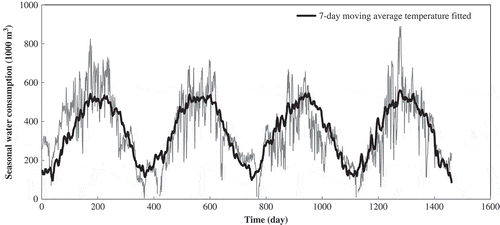
After subtracting the base water consumption, water consumption was regressed with the 7-day moving average temperature value, which can reduce the randomness of daily temperature and results in sinusoidal variation within 1 year, similar to seasonal water consumption. Therefore, the linear fitting formula between seasonal water use and the corresponding 7-day moving average temperature was adopted. The seasonal water consumption can be formulated as:

(11)

Seasonal consumption obtained through equation (11) comprises 16% of total water consumption and reflects more than 60% of seasonal variation, which indicates that taking the 7-day moving average temperature as an independent variable can capture the nature of the seasonal component, as shown in Fig. 4. Water consumption is found to linearly increase with average temperature at the rate of 12.9 × 10³ m³ per °C. We also adopted DFT to investigate this seasonal component, but the performance was poor. This poor performance can be attributed to the fact that the method used in this article can adjust the temperature pattern for each year, whereas DFT uses a fixed procedure for any year.

Fig. 4 The 7-day moving average temperature fitted and daily mean seasonal water consumption in Beijing (2006–2009).

Daily meteorological effect

A multivariate threshold regression model developed by Yan and Cao (1994) was introduced to describe the complex nonlinear correlation between daily meteorological data and water consumption. Daily maximum temperature and precipitation were considered, and the results indicate that the occurrence of precipitation has a more significant impact on this part of water use. The threshold value of precipitation of 0 mm (F-value: 281) and daily maximum temperature of 31.1°C (F-value: 187) are significant at the 5% level via the F-test. Moreover, the factor with a larger F-value indicates a more significant effect on water use. This component is mainly affected by the daily meteorological variation and can be formulated as:

(12)

Habitual component

The habitual consumption equation, derived via stepwise regression analysis with the p-value of every coefficient less than 1%, is expressed as follows:

(13)

where represents the habitual water consumption of the current day, and d – 1, d – 2 and d – 7, respectively, stand for 1, 2 and 7 d before the current day.

Validation of daily water consumption

Daily water consumption is estimated as the sum of the base, seasonal and habitual water components. From 2006 to 2009, the comparison between estimated and recorded data in terms of R², AARE and TS_x (x = 1, 3, 5, 10, 15) are listed in Table 1. Figure 5(a) shows the histogram of the relative errors of daily water-use estimation. We find that 82% of model estimates fall within the relative error band of ±3%, whereas 94% fall within ±5%. The normality in error estimates also indicates that the model performs well. The comparison between the estimated daily and observed total water consumption is shown in Fig. 5(b), and a very good match is obtained, with R² = 92.5%.

Fig. 5 (a) Relative errors of daily water consumption calibration in Beijing main district (2006–2009; dark-shaded bars are in the 3% error band) and (b) comparison between observed and estimated daily water consumption in Beijing main district (2006–2009).

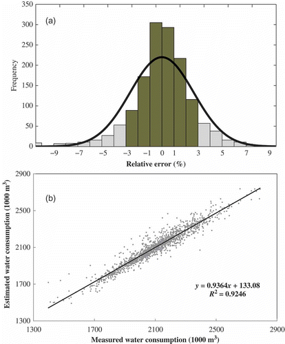
Table 1 Statistics in the calibration and validation periods (%).

	R^2	AARE	TS1	TS3	TS5	TS10	TS15
Calibration period	92.46	1.85	41.40	81.91	94.15	99.17	99.79
Validation period	90.16	1.80	41.06	84.08	95.25	98.88	99.72

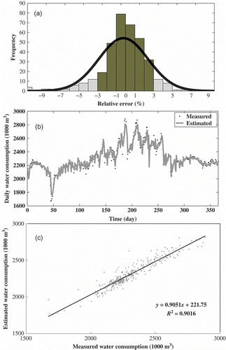
The forecasting capability of the developed model was tested using the data set from 1 January 2010 to 31 December 2010, including water-use information and observed weather data. As shown in Fig. 6(a), 84% of the daily estimates are within the error band ±3%, whereas 95% are within ±5%. Figure 6(b) and (c) indicates that the modelled daily urban water consumption matched the recorded water use well in terms of both amount and process.

Fig. 6 (a) Relative errors of daily water consumption validation in Beijing (2010; dark-shaded bars are in the 3% error band); (b) comparison of measured and estimated daily water consumption in Beijing from 1 January 2010 to 31 December 2010 and (c) comparison between measured and estimated daily water consumption in Beijing (2010).

DISCUSSION

This study focused on the modelling of daily water consumption of Beijing main district, and good performance was achieved for the period 2006–2009. A series of statistical models was adopted to interpret daily water-use variation in Beijing.

From the result of the base component, we note that base water consumption of Beijing increases at a rate as high as 280 m³ d^-1, which is approximately 2.6 times greater than that of Hong Kong (Wong et al. 2010). As previously mentioned, the base component can be attributed to a combination of social and economic factors. Quantifying the contributions of each factor to this component is difficult. However, by comparing the situations of Hong Kong and Beijing, we find that the GDP growth of the city is apparently in harmony with the increasing rate of base water use. From 1990 to 2001, the model period of the base component of Hong Kong, annual GDP growth was approx. 4.5%, excluding the impact of the Asian financial crisis of 1997 to 1998 (The World Bank 2012). Likewise, the annual GDP growth of Beijing was 11.6% during the model period of 2006–2009 (Beijing Municipal Bureau of Statistics 2011), which is approx. 2.6 times the growth of Hong Kong, and in agreement with the ratio of base water use increase rate between Beijing and Hong Kong. This agreement indicates the possibility of an essential contribution by GDP growth to base water consumption growth and that introducing the GDP growth factor may be more effective when estimating urban base water use.

The seasonal component reflects daily urban water consumption at the seasonal scale and varies as a result of local prevailing weather. The threshold regression model in equation (12) indicates that the occurrence of precipitation is more sensitive than the occurrence of maximum temperature. The occurrence of precipitation results in a step change in water-use response. Statistically, this component decreases by 3.52 × 10³ m³ with 1 mm precipitation increment, whereas the average 1°C rise in maximum temperature can result in approximately 1.6 × 10³ m³ more water consumption, regardless of whether a rainfall event occurs. This seasonal use pattern is consistent with Beijing’s climatic characteristics—semi-arid with less precipitation in recent years. We believe that a sizable part of seasonal water use is for outdoor purposes, such as garden watering, which decreases more sensitively when precipitation occurs compared with the decrease in maximum temperature. Therefore, although the magnitude may be low, sizable variation in local climatic conditions, such as less frequent but more intensive precipitation (Liu et al. 2005), has an effect on the local water demand pattern.

The effect of the day of week on water-use persistence is illustrated in the habitual component. People in cities have a weekly life and work cycle. Therefore, the 7-day period yields the habitual water-use pattern. The daily water use of one day, two days and a week ago has a more significant correlation with the current day’s water use than water use of any other days. The p-values of these three items’ coefficients are all at least three orders of magnitude smaller than others. The inertia of water-use behaviour is found for the previous two days, with the closer date having more significant persistence. Moreover, the major factor influencing the current day’s habitual use in Beijing is water use of one day ago, followed by seven days ago, as indicated by the magnitude of the coefficients in equation (13).

This analysis could potentially be improved if more daily water-use data were available and more reasonable assumptions were to be employed. The assumption that base water consumption increases linearly is worth reconsidering under a rapidly changing environment or long-term conditions. The substantial increase in water demand attributed to population growth and per-capita water use induced by economic development, in addition to the effects of climatic change on water availability, may be more appropriately described by a nonlinear relationship over time instead of a linear equation (Vairavamoorthy et al. 2008). The linear compromise was made considering only five years of recorded daily water consumption data. Another improvement could be made by dividing the study area into smaller districts in terms of spatial heterogeneities, when using such a tool (Sempewo et al. 2008).

CONCLUSIONS

In this study, a statistical model is proposed for the estimation of daily urban water consumption. Total water use is decomposed into the base, seasonal and habitual components; each component is mainly affected by various factors and estimated using different methods. The model was applied to analyse urban water consumption in the Beijing central urban area, and it achieved good performance. With the aid of this model, we can interpret the structure of daily urban water and its impact factors at different time scales, while also providing a real-time forecast of daily water use.

Although fairly good results were obtained in this study, future research efforts are recommended, including a model with a more physical mechanism to estimate base consumption and consideration of more factors in the multivariate and multi-threshold regression.

Acknowledgements

We thank the Beijing Water Authority and the Beijing Climate Observatory for the water use and meteorological data.

Funding

This research was supported by the National Natural Science Foundation of China [grant number 51190092), the Ministry of Science and Technology of China [Project no. 2011BAC09B07] and the Beijing Municipal Science and Technology Committee [Project no. D101106047210001].

REFERENCES

- Arbues, F. and Villanua, I., 2006. Potential for pricing policies in water resources management: estimation of urban residential water demand in Zaragoza, Spain. Urban Studies, 43 (13), 2421–2442.
- Beijing Municipal Bureau of Statistics, 2011. Beijing statistical yearbook. Beijing: China Statistics Press.
- Beijing Water Authority, 2009. Beijing water resources bulletin. Beijing: Beijing Water Authority.
- Bougadis, J., Adamowski, K., and Diduch, R., 2005. Short-term municipal water demand forecasting. Hydrological Processes, 19 (1), 137–148.
- Brookshire, D.S., et al., 2002. Western urban water demand. Natural Resources Journal, 42 (4), 873–898.
- CASS (Chinese Academy of Social Sciences), 2010. Annual report on urban development of China. Beijing: CASS.
- CASS (Chinese Academy of Social Sciences), 2011. Annual report on analysis of Beijing society-building. Beijing: CASS.
- Dalhuisen, J.M., et al., 2003. Price and income elasticities of residential water demand: a meta-analysis. Land Economics, 79 (2), 292–308.
- Gato, S., Jayasuriya, N., and Roberts, P., 2007. Temperature and precipitation thresholds for base use urban water demand modelling. Journal of Hydrology, 337 (3), 364–376.
- House-Peters, L.A. and Chang, H., 2011. Urban water demand modelling: review of concepts, methods, and organizing principles. Water Resources Research, 47 (5), W05401.
- Kowalczak, P. and Kundzewicz, Z.W., 2011. Water-related conflicts in urban areas in Poland. Hydrological Sciences Journal, 56 (4), 588–596.
- Liu, B., et al., 2005. Observed trends of precipitation amount, frequency, and intensity in China, 1960–2000. Journal of Geophysical Research, 110 (D8), D08103.
- Maidment, D.R., Miaou, S.P., and Crawford, M.M., 1985. Transfer function models of daily urban water use. Water Resources Research, 21 (4), 425–432.
- Miaou, S.P., 1990. A class of time-series urban water demand models with nonlinear climatic effects. Water Resources Research, 26 (2), 169–178.
- Miaou, S.P. and Maidment, D.R., 1986. Daily water use in nine cities. Water Resources Research, 22 (6), 845–851.
- Protopapas, A.L., Katchamart, S., and Platonova, A., 2000. Weather effects on daily water use in New York City. Journal of Hydrologic Engineering, 5 (3), 332–338.
- Richard, C.C. and Parker, A., 2009. Climate change, population trends and groundwater in Africa. Hydrological Sciences Journal, 54 (4), 676–689.
- Schleich, J. and Hillenbrand, T., 2009. Determinants of residential water demand in Germany. Ecological Economics, 68 (6), 1756–1769.
- Sempewo, J., Pathirana, A., and Vairavamoorthy, K., 2008. Spatial analysis tool for development of leakage control zones from the analogy of distributed computing. In: Proceedings of the 10th annual water distribution system analysis conference (WSDA 2008), 17–20 August. Kruger: American Society of Civil Engineers (ASCE), 676–690.
- The World Bank, 2012. GDP growth (annual %) [online]. Available from: http://data.worldbank.org.cn/indicator/NY.GDP.MKTP.KD.ZG [Accessed 27 February 2013].
- Tong, H., 1983. Threshold models in non-linear time series analysis. Lecture notes in statistics, No. 21. New York: Springer-Verlag.
- Vairavamoorthy, K., Gorantiwar, S.D., and Pathirana, A., 2008. Managing urban water supplies in developing countries—climate change and water scarcity scenarios. Physics and Chemistry of the Earth, Parts A/B/C, 33 (5), 330–339.
- Wong, J.S., Zhang, Q., and Chen, Y.D., 2010. Statistical modelling of daily urban water consumption in Hong Kong: trend, changing patterns, and forecast. Water Resources Research, 46 (3), W03506.
- Worthington, A.C. and Hoffman, M., 2008. An empirical survey of residential water demand modelling. Journal of Economic Surveys, 22 (5), 842–871.
- Yan, H. and Cao, J., 1994. Method of building a multivariate threshold regression model. Chinese Journal of Atmospheric Sciences, 18 (2), 194–199.
- Zhou, S.L., et al., 2000. Forecasting daily urban water demand: a case study of Melbourne. Journal of Hydrology, 236 (3), 153–164.