Projection of future world water resources under SRES scenarios: an integrated assessment

Abstract

Changes in water resources availability, as affected by global climate warming, together with changes in water withdrawal, could influence the world water resources stress situation. In this study, we investigate how the world water resources situation will likely change under the Special Report on Emissions Scenarios (SRES) by integrating water withdrawal projections. First, the potential changes in water resources availability are investigated by a multi-model analysis of the ensemble outputs of six general circulation models (GCMs) from organizations worldwide. The analysis suggests that, while climate warming might increase water resources availability to human society, there is a large discrepancy in the size of the water resource depending on the GCM used. Secondly, the changes in water-stressed basins and the number of people living in them are evaluated by two indices at the basin scale. The numbers were projected to increase in the future and possibly to be doubled in the 2050s for the three SRES scenarios A1b, A2 and B1. Finally, the relative impacts of population growth, water use change and climate warming on world water resources are investigated using the global highly water-stressed population as an overall indicator. The results suggest that population and socio-economic development are the major drivers of growing world water resources stress. Even though water availability was projected to increase under different warming scenarios, the reduction of world water stress is very limited. The principal alternative to sustainable governance of world water resources is to improve water-use efficiency globally by effectively reducing net water withdrawal.

Editor Z.W. Kundzewicz; Associate editor D. Gerten

Résumé

Les modifications de la disponibilité des ressources en eau dues au réchauffement climatique, ainsi que les modifications des prélèvements d’eau, pourraient influencer le stress des ressources en eau mondiales. Dans cette étude, nous examinons comment la situation des ressources en eau mondiales serait susceptible de changer dans le cadre du Rapport spécial sur les scénarios d’émissions (SRES) si l’on y intègre des projections de prélèvements d’eau. Tout d’abord, les changements potentiels de la disponibilité des ressources en eau ont été examinés par une analyse multi-modèle des sorties de l’ensemble de six modèles de circulation générale (MCG) de différentes organisations. L’analyse a suggéré que, si le réchauffement climatique pourrait accroître la disponibilité des ressources en eau pour les sociétés humaines, il y a de grandes différences sur cette disponibilité selon le MCG utilisé. En second lieu, les changements dans les bassins soumis au stress hydrique et le nombre de personnes vivant dans ces bassins ont été évalués par deux indices à l’échelle du bassin. Ces chiffres devraient augmenter à l’avenir et peut-être doubler dans les années 2050 pour les trois scénarios SRES A1b, A2 et B1. Enfin, les impacts relatifs de la croissance démographique, des modifications de l’utilisation de l’eau et du réchauffement climatique sur les ressources en eau mondiales ont été étudiés en prenant comme indicateur global la population mondiale soumise à un important stress hydrique. Les résultats suggèrent que l’importance de la population et le développement socio-économique sont les principaux moteurs de l’accroissement du stress hydrique à travers le monde. Même si la disponibilité de l’eau devait augmenter selon différents scénarios de réchauffement, la réduction du stress hydrique dans le monde serait très limitée. La principale stratégie permettant de réaliser une gouvernance durable des ressources en eau mondiales consiste à améliorer l’efficacité de l’utilisation de l’eau à l’échelle mondiale en réduisant effectivement les prélèvements d’eau nets.

Key words:

• climate warming
• water resources availability
• water stress
• GCM
• SRES
• climate warming impacts
• population and economic development impacts
• global

Mots clefs:

• réchauffement climatique
• disponibilité des ressources en eau
• stress hydrique
• MCG
• SRES
• effets du réchauffement climatique
• impacts de la population et de développement économique
• échelle mondiale

INTRODUCTION

For world water resources assessment, as well as the projection of water withdrawal in the future, it is important to forecast future water resources availability including their volume and variability in time and space. In addition to the pressure from societal demand, water resources systems are also affected by the pressure from climate change. There is common recognition that global warming due to accelerating greenhouse gases concentration in the atmosphere is likely to have significant effects on the hydrological cycle and water resources (e.g. Houghton et al. 1996, IPCC 2001, 2007).

Several studies have addressed the intensification of the global hydrological cycle and indicated that more water resources will be available to human society (e.g. Arnell 2004, Oki and Kanae 2006). More important than the increase in global runoff to water resources systems, however, is the uneven distribution of the potentially increased water resources across the world. The recent Assessment Reports of the Intergovernmental Panel on Climate Change (IPCC) warned that global warming is likely to lead to increases in both floods and droughts.

Generally, hydrologists translate the climate forecasts by general circulation models (GCM) to projections of the long-term availability of water resources in future. However, GCM forecasts of runoff change are largely dependent on the climate forcing, model dynamics and parameterization; e.g. one model may predict that a region will possibly become wetter, but another model may give the completely opposite forecast. Until now most studies on world water resources assessment have been based on specific, or a limited number of, GCMs (e.g. Vorosmarty et al. 2000, Oki et al. 2001, Alcamo et al. 2003, 2007). Recently, several attempts using multi-model ensemble analysis technologies to reduce the model-specific uncertainty in the evaluation of potential change in hydrological systems due to climate warming were reported (e.g. Nohara et al. 2006, Tebaldi et al. 2006). Murray et al. (2012) used a global vegetation model to evaluate the climate warming impacts on global water resources at the end of the 21st century. Based on an analysis of the extractions in four semi-arid to arid basins, Grafton et al. (2013)  pointed out that although climate change could bring more water resources to those basins, over extraction plays a determinant role in reducing the water system flow; therefore, they suggested that the water governance should be urgently changed to adapt to climate change.

In the context of world water resources assessment under the scenarios described in the Special Report on Emissions Scenarios (SRES) of IPCC (Nakicenovic and Swart 2000), Arnell (2004) used six GCMs to give an assessment of the future change in water resources and population living in water scarce basins by using the water scarcity index (Q/c, defined later in the “Water stress indices” section). Alcamo et al. (2007) used climate inputs from two European GCMs (ECHAM4 and HadCM3) to drive a global hydrological model and analysed the water stressed basins and population with three indicators for the SRES A2 and B2 scenarios.

In this study, we present an integrated assessment of the potential change in global water resources by integrating both the projections of future water withdrawal (Shen et al. 2008) and water resources availability using consistent climate and socio-economic scenarios, SRES. To enable comparisons with the above mentioned studies (Arnell 2004, Alcamo et al. 2007), we use the same time slices. Although Arnell (2004) presented the situation by using six GCMs he did not consider the impact of socio-economic development such as water withdrawal. Alcamo et al. (2007) evaluated water withdrawal effects using two models but only for two scenarios, and the two GCMs (ECHAM4 and HadCM3) employed show large differences in performance compared to other models in our investigation. Therefore, this study attempts to give a comprehensive assessment by overcoming the shortcomings of both the precedent studies.

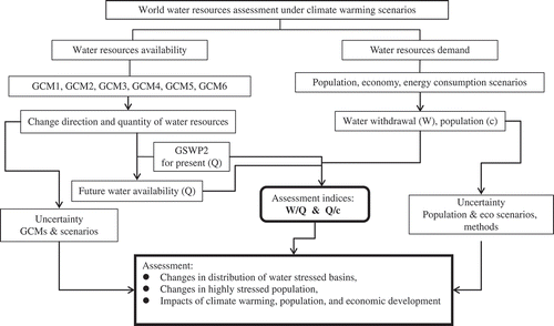
The paper presents the multi-GCM analysis of the potential change in water resources availability. The GCM outputs of runoff were calculated on a coarser grid (see Table 1) and linearly interpolated to a 0.5-degree resolution. Then we calculated the global and regional population declines in water-stressed basins, and evaluated the impacts of population, water use and climate warming on the water resources system. The primary aim of this paper is to provide and enhance information on future world water resources as part of the activities sponsored by the IPCC and to contribute to climate change assessment.

METHODOLOGY

Climate data and processing

The simulation results for three IPCC SRES scenarios, A1b, A2, and B1, produced by six GCM models from different organizations across the world were selected to analyse the freshwater resources availability due to climate warming. All of the GCM outputs are provided by the Program for Climate Model Diagnosis and Intercomparison (PCMDI). Due to the lack of the outputs for the SRES B2 scenario in the PCMDI data archive (at https://esg.llnl.gov:8443/index.jsp, last access 25/10/2006), we could not assess the water resources situation change for that scenario. Table 1 shows the details of the six GCM models, which were selected based on our previous investigation of their performances in the 20th century experiment simulation (20c3m, see IPCC 2007). We compared the global mean precipitation from 19 GCMs’ outputs with ground observation based data from the Global Precipitation Climatology Project (GPCP) and selected the six GCMs according to their deviations relative to the GPCP dataset. The various original spatial resolutions of the models outputs, i.e. total runoff, were interpolated linearly to global grid cells at 0.5-degree resolution.

Table 1 Descriptions of climate forecasting data used for water resources analysis.

Model name	Short name	Organization	Original resolution
Current (1986–1995)
Multi-model	GSWP2	GEWEX/GSWP2	1° × 1°
Future (2000–2100)
GISS-ER	GISSer	NASA/Goddard Institute for Space Studies, USA	5.0 × 4.0
MIROC3.2-Med	MIROC3	CCSR/NIES, Japan	T42L20
MPI-ECHAM5	ECHAM5	Max Planck Institute for Meteorology, Germany	T63L31
MRI-CGCM2.3.2a	CGCM2	Meteorological Research Institute, Japan	T42L30
NCAR-CCSM3.0	CCSM3	National Center for Atmospheric Research, USA	T85L26
UKMO-HadCM3	HadCM3	Hadley Centre for Climate Prediction and Research, MetOffice, UK	2.5 × 3.75L19

The outputs for runoff of the six GCMs were employed for estimating the future potential change in water resources supply. First, we averaged the 30-year GCM predictions at each time slice to minimize the inter-annual variability. The average of 1970–1999 was used for the present time slice, 2010–2039 for the 2020s, 2040–2069 for the 2050s, and 2060–2089 for the 2070s. Then, the differences of annual runoff simulated by each GCM for the 0.5-degree grids in the 2020s, 2050s and 2070s, relative to the present time slice, were treated as the change of water resources due to global warming. To obtain the spatial distribution of future runoff, these changes are then added to the 10-year mean runoff data of the Global Soil Wetness Project 2 (GSWP2) multi-model products, which were generated by an ensemble mean of 13 land surface models (LSMs) from various worldwide organizations using a unique forcing dataset (see Diemeyer et al. 2006). The multi-model product of GSWP2 has been widely used for analysing global hydrological cycles and water balance (Oki et al. 2005) and is treated as the water availability in the present time slice.

Multi-model analysis of potential change in available freshwater resources

Through multi-model analysis we can enhance our confidence regarding the regions/basins showing consistency in the change directions of water supply among different GCMs and, at the same time, understand the regions with largely uncertain change directions and their problems.

The method of multi-model analysis is simple. We first calculated the basic statistical parameters of each grid, such as the simple ensemble mean, standard deviation and coefficient of variation (Cv) of the 30-year mean runoff, with bias correction, in future time slices of the six ensemble members. For the bias correction, we calculated the difference of each GCM’s output between the future time slice and the reference time slice, i.e. 1970–1999, and added this difference or “change” to the results of GSWP2 to obtain the bias-corrected future water availability. Then the grid-scale variability of runoff among the six GCMs was evaluated by Cv to identify the grids where the consistency of the forecast runoff simulated by the six GCMs was significant or insignificant. In other words, if the Cv of one grid is larger than a threshold value (set at 0.1), the consistency of future runoff simulated by the six models at that grid will be insignificant or of low confidence, and vice versa. Finally, we calculated the change rate of the simple ensemble mean of future runoff against the current runoff, presented by the GSWP2 multi-model dataset, of each grid and classifed the results into four categories: increase with high confidence, decrease with high confidence, no-change with high confidence, and change amplitude/direction uncertain. The classification criterion is 5% change against the current runoff. If the increase (or decrease) in runoff is more than 5%, the grid is classified as increase (or decrease) with high confidence; if the change in runoff is less than 5%, the grid is classified as no-change with high confidence or change subtle. The change amplitude/direction for grids where the result is uncertain are not classified.

The detailed description of the method in mathematical form can be seen in the Appendix to this paper.

Development of datasets of population and water withdrawal for different scenarios

We separately developed gridded datasets for global population (Bengtsson et al. 2006b) and water withdrawal (Shen et al. 2008) under the socio-economic conditions prescribed in SRES scenarios. The population dataset was created based on the current distribution of rural and urban population projected by the UN and the population growth rate of each country projected by SRES. The total water withdrawal was obtained by integrating the separate estimations of agricultural, domestic and industrial withdrawals (see Shen et al. 2008 for details). Agricultural withdrawal was estimated through multiplying the irrigated land area by irrigation intensity. The irrigated land was assumed to be proportionally related to population change of each country and limited by geomorphologic factors and the necessary residential land occupied in each grid. Domestic withdrawal was estimated by analysing the relationship of per capita GDP and per capita daily domestic water use, and extrapolating the relationship to the future using the population data and GDP projections in SRES. Industrial withdrawal was estimated by scaling the present industrial use with the growth rate of industrial electricity consumption and an improvement coefficient of industrial water-use efficiency, which was assumed equal to the improvement coefficient of energy use for unit GDP (Shen et al. 2008).

Since its publication, the water withdrawal dataset has been much used by researchers worldwide in different fields, such as ecological conservation (FitzHugh et al. 2012), electricity generation demand (Davies et al. 2013), environmental flow (Deitch et al. 2012) and climate adaptation cost (Martín-Ortega 2011).

Water stress indices

We assess the world water resources situation from the perspective of water stress, which usually reflects the overall pressure put on water resources. Two water stress indices are widely used. One popular is the so-called withdrawal-to-availability ratio, defined as the annual water withdrawal divided by annual water availability at the basin scale, W/Q, where the W is annual freshwater off-stream withdrawal for agricultural, industrial and domestic sectors, and Q is annual renewable freshwater resources (e.g. Falkenmark et al. 1989, WMO 1997, Vorosmarty et al. 2000). Usually, the extent of water stress is categorized as no-stress (W/Q < 0.1), low stress (0.1 < W/Q < 0.2), moderate stress (0.2 < W/Q < 0.4), and high stress (W/Q > 0.4). This classification was used by WMO (1997), Vorosmarty et al. (2000), Alcamo et al. (2003, 2007), Cosgrove and Rijsberman (2000), and Oki et al. (2001). This index has the advantage of reflecting the integrated effects of both the pressure from human society (the demand side) and hydrological system (the supply side).

Another widely used indicator is the water scarcity index, defined as per capita water availability (Q/c, annual freshwater resource Q divided by population, c, at river basin scale, in m³ c^-1 year^-1 ). The water scarcity index Q/c is the inverse of the original Falkenmark water crowding indicator (the number of people sharing one flow unit of blue water, Falkenmark and Rockström 2004). We adopt the commonly used classification of water stress extent: no stress (Q/c > 1700 m³ c^-1 year^-1), moderate stress (1000 < Q/c < 1700 m³ c^-1 year^-1), and high stress (Q/c < 1000 m³ c^-1 year^-1). Sometimes, a river basin with Q/c less than 500 m³ c^-1 year^-1 is classed as being under extreme stress. Many studies have used these criteria (e.g. Arnell 1999, 2004, Alcamo et al. 2003, 2007, UNEP 2004, Oki and Kanae 2006, Arnell et al. 2011, Parish et al. 2012). The advantage of the Q/c index is its simplicity; it needs only population and water availability, but it cannot reflect other factors influencing the water resources situation, e.g. water use and management technologies.

In this study, we assess the extent of water stress globally using these two indices at the basin scale. We can quickly obtain a rough impression of change in water resources status using Q/c and compare with existing studies, e.g. Arnell (2004), even though it cannot reflect the influence of economic development well. Through the W/Q index we can analyse the more detailed effects of population and economic development on the water resources system. Some uncertainty will definitely be raised due to the methodology for withdrawal estimation, but it has the advantage of providing insight to the effects of different population, economics and climate factors.

The demand data used were from our former estimation of the global distributions of population (Bengtsson et al. 2006b) and water withdrawal (Shen et al. 2008), which were combined with the water availability projections to make the assessment. Figure 1 shows the technical routing of the data used and the calculation method for water resources assessment.

Fig. 1 Schematic of technical routing and data processing in this study.

WATER RESOURCES AVAILABILITY

Present freshwater resources availability

The freshwater resources available at present are estimated by the multi-model ensemble products of GSWP2, as mentioned earlier. GSWP2 was an attempt to reconstruct the global hydrological cycle during 1986–1995 through 14 land surface schemes (LSMs) from various research organizations over the world (Dirmeyer et al. 2006). The present global hydrological cycle and water resources obtained using GSWP2’s multi-model dataset are presented by Oki and Kanae (2006).

The present water resources produced by GSWP2 are aggregated in different regions and compared with previous studies. The global total water resource in GSWP2 is 46 000 km³/year. This figure is slightly higher than that presented in Oki and Kanae (2006), 45 500 km³/year, because the latter excluded the amount of water flow into inland basins and only accounts for direct discharges to ocean. Table 2 shows the comparison with present water resources used by Shiklomanov (2000) and Vorosmarty et al. (2000) for eight regions and the world. In general, the world available water resource of GSWP2 is higher than the other two studies. A detailed evaluation of the different runoff datasets (Hanasaki 2006) shows that the water resource in high latitude regions of the Northern Hemisphere is greater in GSWP2 than the other two studies, whilst the water resource of other parts seems not largely different to the others. The later part of this paper illustrates that severely water stressed regions are distributed in the low- to mid-latitudes; therefore, we judged the GSWP2 runoff data to be applicable for this study.

Table 2 Comparison of the current water resources by GSWP2 with previous studies in eight regions and for the world (in km³/year).

Region	GSWP2	Shiklomanov (2000)	Vorosmarty et al. (2000)
N. America	8 000	6 800	5 900
L. America	11 400	13 100	11 700
Europe	3 800	2 900	2 800
M. East + N. Africa	470	500
Sub-Saharan Africa	5 200	4 000
CIS	6 500	3 400	18 200
Asia	9 100	9 700
Oceania	1 600	2 400	700
World	46 070	42 800	39 300

Change direction of available freshwater resources in future

At the global scale, the annual water availability will be likely to increase due to climate warming; the differences between the six models’ results at the global scale range from 3000 to 5000 km³/year, which accounts for 7–11% of the total terrestrial runoff.

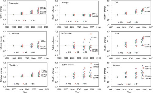
At the regional scale the change trends of water resource forecasts by the six GCMs show large differences (Fig. 2). All six models project that water resources in Northern America and the CIS (Commonwealth of Independent States) will be likely to increase and the range of increase among the GCMs is 5–10%. However, for other regions, some models predict the water resource will increase, while other models predict a decreasing trend (Fig. 2), particularly in Latin America, the Middle East and Africa. Most models suggest water resources availability is likely to decrease in Europe; while, in Asia, Oceania and Sub-Saharan Africa most models forecast that water resources will likely increase. The names of the GCMs that give the maximum or minimum forecast in each region are labelled in Fig. 2.

Fig. 2 Projected changes in water resources availability in eight regions and the world by the six GCMs. The names of the models giving highest and lowest projections are marked next to the points for the 2070s.

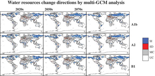
Figure 3 shows the spatial distributions of water resource change direction by multi-model analysis for the three SRES scenarios in the 2020s, 2050s, and 2070s, respectively. Most areas with significant increasing trends are distributed in the boreal regions, central Africa, India, South China and Indonesia. The eastern USA, most of Europe, and some parts of South America show subtle change in annual runoff in future. The European countries near the Mediterranean Sea are likely to become drier in future compared to the present. There are large areas in the semi-arid to arid regions of North China, central Asia, the Middle East, Sahel, East and South Africa, western USA, and inland Australia that show higher uncertainty in the change directions, i.e. different models give completely different change directions.

Fig. 3 Potential change directions of available water resources (total runoff) under A1b, A2 and B1 SRES scenarios as simulated by the 6 GCM models in 2020s, 2050s, and 2070s, respectively. SI indicates a significant increasing trend, SD a significant decreasing trend, and MC a subtle change. The area with UC or white shows large uncertainty in change directions among the different GCMs.

WATER STRESSED BASINS AND POPULATION

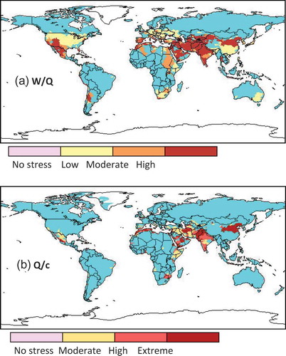
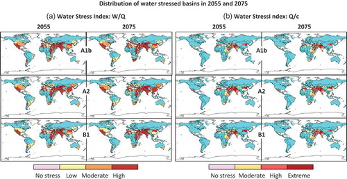
Figure 4 illustrates the present distribution of water stressed basins determined by the two indices. According to the W/Q index, the most water-stressed basins at present are in North China, Central to Western Asia, North Africa, most parts of India and Pakistan, South Africa, southwest USA, Mexico, Chile and southern Europe. The distribution of highly water-stressed basins measured by the Q/c index is less extensive than that by W/Q, indicating that water use and economic factors are definitely important in water resources assessment.

Fig. 4 Distributions of basins with various extents of water stress as defined by the two indices: (a) W/Q and (b) Q/c, in the present time slice.

The water-stressed basins defined by W/Q show an obvious trend of possible enlargement or becoming more severe in the 2050s and 2070s (Fig. 5(a)). The index of Q/c also shows an enlargement trend of highly water stressed basins in Western Asia and Africa, whilst the extent of water scarcity in North China is likely to be mitigated in scenarios A1b and B1 (Fig. 5(b)). This indicates that the increase of population in China is slower than the increase of water resources due to climate warming.

Fig. 5 Distribution of future water stressed basins as defined by W/Q and Q/c in the 2050s and 2075s. The multi-model ensemble mean of discharge was used as the water resource availability (Q).

We calculated the population living in highly water-stressed basins and its change in different regions and the whole world. Our analysis shows that the present population with severe water shortage problems is about 1.75 billion worldwide, as measured by index Q/c (less than 1000 m³ c^-1 year^-1). This figure will likely increase to 3.08–3.66 billion in the 2020s, 3.59–6.22 in 2050s, and 2.73–7.39 billion in the 2070s depending on the different scenarios and climate models. Note that, the highly water-stressed population for the A1b and B1 scenarios will decrease in the 2070s compared to the the 2050s due to population decrease and water resource increase by climate warming, but this is not so for the A2 scenario.

If socio-economic factors are accounted for, the population living in highly water-stressed basins is currently 2.53 billion according to the index W/Q (as greater than 0.4 at basin scale). This figure will also be likely to increase to 3.62–4.76 billion in the 2020s, 4.16–7.58 billion in 2050s, and 3.80–8.91 billion in the 2070s. The highly-stressed population in the 2070s for scenario B1 is also lower than that in the 2050s depending on the scenario and climate model.

Figure 6 illustrates changes in the ratio of world population living in highly water-stressed basins by the two indices. According to the W/Q index, the percentage of highly water-stressed population in the world is currently 41% and will likely reach 54%, 64% and 49% in 2070s under the A1b, A2 and B1 scenarios, respectively. These percentages show the simple ensemble means of the six GCMs. Note that the range between the different GCMs varies from 5% to 10%, depending on the scenario (Fig. 6(a)). The percentages of highly water-stressed population illustrated by the Q/c index are lower than those by W/Q, and likely to change from the current 29% to 40%, 52% and 43% in 2070s for scenarios A1b, A2 and B1, respectively. However, the range amongst different GCM models is fairly large and especially for scenario A1b.

Fig. 6 Current and future projections of highly water-stressed population ratio in the world for scenarios A1b, A2 and B1 measured by (a) W/Q and (b) Q/c. The error bars shows the range caused by water resource projections of different GCMs.

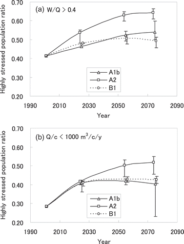
Comparing the A1b and B1 scenario curves for the different indices may help understanding of how the socio-economic factor affects the water supply–demand balance. The highly water-stressed population of the world for B1 is generally larger than that for A1b as measured by the Q/c index (Fig. 6(b)), indicating the freshwater resource projected by the climate models with the B1 scenario is less than for the A1b scenario (note the population is identical for the two scenarios). However, the highly water-stressed population ratio measured by W/Q will likely be higher in scenario A1b than in B1 (Fig. 6(a)) in the 2050s and 2070s. This implies that, even though the water resource in B1 is projected to be less than that in A1b, the significant reduction of water withdrawals globally in the B1 scenario (Shen et al. 2008) works to reduce the water-stressed population.

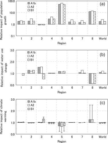
The highly water-stressed population according to index W/Q in each region and the world at present is illustrated in Fig. 7. Asia shares about 73% of the world total, accounting for 1.8 billion people, whilst the numbers for sub-Saharan Africa and Oceania are only 7 and 2 million, respectively. Figure 8 shows the relative change of highly water-stressed population in each region and the world under the three scenarios. The population with severe water scarcity problems in most regions is projected to increase in the future, except for Europe, under scenario B1. Sub-Saharan Africa, the Middle East, North Africa and Latin America show a rapid increase of the highly water-stressed population (Fig. 8), whilst Europe and CIS show a slow increase or even a decrease under scenario B1. The highly water-stressed population in the Middle East and North Africa is likely to increase by three to five fold by the 2070s, depending on scenario.

Fig. 7 The highly water-stressed population of eight regions and the world total at present measured by index W/Q. The numbers above each bar illustrate the total population living in highly water-stressed basins in each region. (1: North America; 2: Latin America; 3: Europe; 4: Middle East & North Africa; 5: sub-Saharan Africa; 6: CIS; 7: Asia; 8: Oceania).

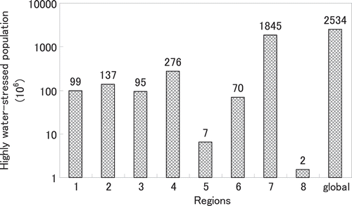
Fig. 8 The relative change of highly water-stressed population against 2000 in three future time slices for different regions and globally. The bar graph illustrates the average of the six GCM models; the error bar shows the range amongst the GCMs. (1: North America; 2: Latin America; 3: Europe; 4: Middle East & North Africa; 5: sub-Saharan Africa; 6: CIS; 7: Asia; 8: Oceania. For Region 5, the change rate was scaled by 0.1).

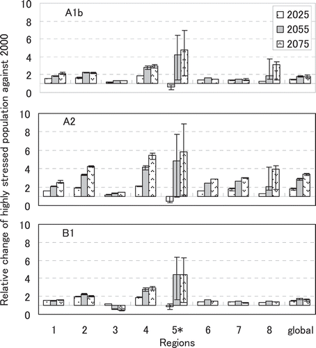
Sub-Saharan Africa shows a decreasing trend in the 2020s and a dramatic increase thereafter, and the ensemble-averaged population with high water stress is projected to be around 40–60 times the present, 7 million by the 2070s. However, the range amongst different GCMs is very large. For example, in the 2070s, under scenario A1b, the highly water-stressed population of sub-Saharan Africa is projected to increase 20-fold by NCAR-CCSM3.0 and 70-fold by the MPI-ECHAM5 model. Large variance amongst GCMs can also be seen in Oceania for the A1b and A2 scenarios (Fig. 8). The future highly-stressed population in Asia is likely to be more than 1.5 times the present number. The world total highly water-stressed population in the 2070s is projected to be less than twice the present number under scenarios A1b and B1, but more than three times that number under scenario A2.

EFFECTS OF CLIMATE WARMING AND SOCIO-ECONOMIC DEVELOPMENT

The change in population living in highly water-stressed basins of the world is a result of the changes in population, water use and climate. To evaluate the effects of these three factors, we calculated the water stress index W/Q and world highly water-stressed population for the following three cases:

• Case 1 represents the population change according to SRES scenarios; both the quantity and distribution of water-use (as withdrawal per capita) and climate conditions (as water resource availability) are fixed at the present status, i.e. without climate and economic change.

• Case 2 represents population and water-use changes but the climate is fixed to the present status, i.e. without climate change. The water-use changes in Case 2 are accounted for by the changes in water withdrawal intensity, which is considered to reflect the changes in economic development.

• Case 3 represents the situation of population, water use (withdrawal) and climate conditions change as prescribed in the SRES scenarios.

The difference between Case 1 and Case 2 can be interpreted as the effect of water use or economic development on water stress, whilst the difference between Case 2 and Case 3 may account for the effect of climate warming.

Population growth and economic development will generally lead to water use increase. However, the net water withdrawal for some countries (especially developed countries) might begin to reduce when water-use intensity reaches its saturation level, or if recycling technology is extensively used (Alcamo et al. 2003). With regard to the effects of climate change, as discussed earlier, the global water resource will likely increase due to climate warming under the A1b, A2 and B1 scenarios. This implies that, at the annual scale, climate warming may make more water available for human society use. As a consequence, water stress might be mitigated at the global scale relative to the situation without climate warming.

Worldwide highly water-stressed population

Table 3 shows the changes in the worldwide highly water-stressed population for the three cases. In the case of population change only, depending on the population growth scenario, the highly-stressed population in the 2020s will increase to 3.5–3.9 billion from 2.5 billion in 2000. The population in highly-stressed basins will account for 45% of the total world population. By the 2050s, the worldwide highly stressed population will be 4.4–6.3 billion, i.e. 47–54% of the world population.

Table 3 Effects of population, socio-economic and climatic changes on worldwide population living in highly water-stressed basins.

			Case 1^a		Case 2		Case 3^d
		World population (10^6)	HSP^b (10^6)	%^c	HSP (10^6)	%	HSP (10^6)	%
2000		6133	2534	41.3	2534	41.3	2534	41.3
2025	A1^b	7935	3593	45.3	3706	46.7	3684	46.4
	A2	8724	3972	45.5	4744	54.4	4653	53.3
	B1	7935	3593	45.3	3789	47.8	3822	48.2
	B2	8042	3644	45.3	3703	46.0	−	−
2055	A1^b	8718	4417	50.7	4764	54.6	4571	52.4
	A2	11791	6330	53.7	7567	64.2	7350	62.3
	B1	8718	4417	50.7	4556	52.3	4423	50.7
	B2	9544	4493	47.1	4776	50.0	−	−
2075	A1^b	8317	4120	49.5	4657	56.0	4495	54.0
	A2	13556	7451	55.0	9011	66.5	8635	63.7
	B1	8317	4120	49.5	4239	51.0	4092	49.2
	B2	10065	5213	51.8	5436	54.0	−	−

^aCase 1 represents the situation with population change only, socio-economic (as water withdrawal intensity) and climatic conditions are fixed to the current level; Case 2 is the situation with population and socio-economic changes but the climate is fixed; Case 3 represents the situation with all the population, socio-economic, and climatic changes.

^bHSP means highly-stressed population.

^cThe columns illustrate what percentage of the increased population against year 2000 will live in highly-stressed basins.

^dThe numbers for Case 3 refer to the multi-GCM ensemble mean.

In Case 2, which considers economic development and consequent change in water withdrawal intensity (withdrawal per capita), the highly-stressed population will generally be greater than that in Case 1, e.g. in the 2050s, 50–64% of the world population will live in basins with severe water scarcity.

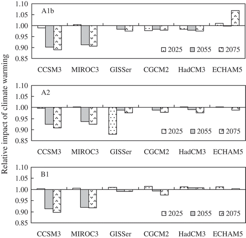
Comparing the number of people living in highly water-stressed basins in cases 2 and 3 suggests that climate warming can generally mitigate the water stress situation to a certain extent, but the absolute population in highly water-stressed basins is still greater than in Case 1. Since the quantity and distribution of water resources forecast by different GCMs show large discrepancies, it is necessary to investigate the performances of the six different GCMs. Figure 9 illustrates how the relative impact of climate warming on water stress varies amongst the different GCMs from the viewpoint of highly-stressed population. For scenario A1b, except for ECHAM5, which forecasts that climate warming will increase the highly water-stressed population across the world (hereafter, we call this a negative effect), the other five GCMs show climate warming could reduce the size of the highly water-stressed population (hereafter, positive effect). For scenario A2, most GCMs forecast a likely positive effect of climate warming. For scenario B1, the HadCM3 and ECHAM5 models see slightly negative effects of climate warming on water stress in the future, whilst the other models see a positive effect after the 2020s. Generally, the CCSM3.0 and MIROC3.2 models show that climate warming could reduce the worldwide highly water-stressed population by around 10% in the 2050s and 2070s for all scenarios; the other models illustrate that the effect of climate warming is rather limited, except for GISS-ER, which projects a significant positive effect in the 2020s for scenario A2, and ECHAM5, which predicts a large negative effect in the 2070s for the A1b scenario. In short, as indicated by the different projections for the number of people living in highly water-stressed basins, the effects of climate warming on water resources are very different depending on GCM. Some models, e.g. CCSM3 and MIROC3, show larger effects at the global scale, but others show smaller effects.

Fig. 9 Relative impact of climate warming on the world population living in highly water-stressed basins by six GCMs in different future time slices. The y-axis denotes the ratio of highly-stressed population in Case 3 to that in Case 2. The ratio of highly-stressed population globally calculated using the present and future water availability for each GCM, and the population and water withdrawal vary according to the scenarios and time slices.

On a regional basis, population growth shows the most significant impacts on water stress extent, as indicated by the number of people living in highly water-stressed basins (Fig. 10(a)). Except for Europe, where the negative population growth has the effect of reducing the highly-stressed population, other regions show large increases in stressed population, especially in sub-Saharan Africa and Oceania, where the highly-stressed population in the 2050s will, respectively, be more than 50 and 10 times the present number. The relative impacts of water use are generally to increase water stress in most regions, except for Oceania where the water-use intensity shows likely significant reductions in the future (Fig. 10(b)). For scenario B1, the water-use changes in North America and Europe also show a large effect of mitigating water stress extent. For the climate warming, a large positive effect (reducing highly-stressed population) is only seen in sub-Saharan Africa; at the same time, significant negative effects (increasing highly-stressed population) are forecast in Europe for scenario B1 and Oceania for scenarios A1b and A2. In the other regions, climate warming shows a very limited effects on the change in population living in highly water-stressed basins (Fig. 10(c)).

Fig. 10 Relative impacts of (a) population, (b) water use and (c) climate on the number of people living in highly water-stressed basins in different regions and the world in 2050s under three different scenarios. Relative impacts are calculated by the ratio of highly-stressed population in Case 1 and 2000; by the ratio of Case 2 and Case 1; and by the ratio of Case 3 and Case 2. (1: North America; 2: Latin America; 3: Europe; 4: Middle East & North Africa; 5: sub-Saharan Africa; 6: CIS; 7: Asia; 8: Oceania).

Water stress extent

Figure 11 shows the impacts of population, water use and climate warming on the water stress extent of world basins in the 2050s. The maps labelled “population only” show the effect of population change on water stress relative to 2000; the water withdrawal per capita per year at each 0.5° grid is relative to the level in 2000. Therefore, the decrease or increase of water stress is completely due to population change. Water stress in the countries of East and South Europe, Russia, China and Japan are mitigated under the A1b and B1 scenarios; in Germany and North European countries there will be no change; and the other countries will suffer increasing water stress due to population increase. For scenario A2, most countries will see increased water stress, except for some European countries and Japan, where the population might not change or even decrease.

Fig. 11 Impacts of population, water use and climate warming on water stress level in the 2050s. Background water stress maps represent the situation after the changes in population, water use and climate change based on index W/Q in the 2050s. By comparing any map with the map to its left, readers can understand which basin will be likely to deteriorate or be mitigated from one class of stress level to another due to the changes in water use or climate warming.

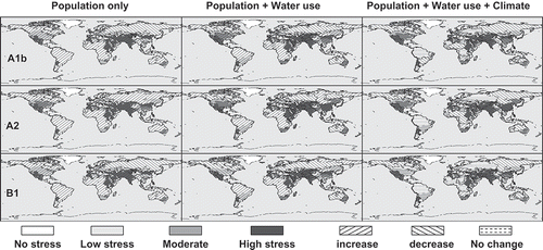
Replacing the water-use intensity (water withdrawal per capita per year) of each grid with the projected value produces the maps labelled “Population + Water use”. Comparing them with those generated by “population change only” one can evaluate the effect of water use (as an integrated result of socio-economic development) on water stress extent. For scenario A1b, the basins in Canada, Russia, Japan, Australia and even Pakistan see a decrease of water stress due to improvement in water-use efficiency. Some basins in southern Canada, Europe, and the southeast of Australia seem unlikely to change much. The water stress situation in the rest of the world is likely to increase due to increasing water use. Some basins in North America, South Africa and East China may change from low to moderate stress. For scenario A2, the trend is nearly the same as for A1b. However, the likely decrease of water stress in Pakistan and East Africa (the Nile basin) might be caused by the substantial decrease of per capita GDP due to fast population increase, which results in per capita water withdrawal decreasing to a level lower than in 2000. As a result, the total water withdrawal in these basins is less than calculated in Case 1. Due to extreme population growth in scenario A2, many basins join the highly-stressed list in the 2050s. The USA seems not to change much. For scenario B1, the water stress of all the developed countries will likely decrease due to improvement of water-use efficiency. The situation in countries in Asia, Africa and Latin America is likely to become more severe due to the increased water use.

The impacts of climate warming are a main concern; however, as discussed earlier, the future climate forecasts are largely dependent on the GCMs’ dynamics and parameterization. At the macro scale, even though most models forecast positive effects of climate warming in reducing the highly stressed population, some models still forecast a future with a slightly deteriorated situation (Fig. 9). Therefore, it is necessary to investigate where and how the climate warming affects the water resources budget. The maps in the right column of Fig. 11 show the simple ensemble mean of the six GCMs, but their forecasts are largely divergent in some regions (see Fig. 3). In other words, there is large uncertainty in the projection of future water resources availability in those areas.

Using the six-GCM ensemble projection, the water stress extents of basins in northern Canada, East Russia, China, India, East Africa and Australia are likely to decrease due to climate warming, whilst those located in the western USA and Mexico, southern South America, around the Mediterranean Sea and in South Africa seem likely to increase. In the remaining areas, the change seems minor. However, most basins seem unlikely to change from one water stress class to another, e.g. from moderate to high stress or vice versa, except for some small basins in the western USA, which will join the highly water-stressed basins group, and the basins in Ethiopia will be likely to become moderate stress from high stress under all three climate warming scenarios. The Brahmaputra basin will likely change from moderate stressed basin to low stress under scenario A1b. This suggests that very few basins will likely change their water stress classification due to climate warming.

The discussions above indicate that population and socio-economic development are the major drivers causing the worldwide water scarcity situation to become more severe. Vorosmarty et al. (2000) proposed a similar argument on this point. Although climate warming might make more water resources available to human society, most basins will be unlikely to change their water stress extent dramatically. In this sense, one of the biggest challenges for human society still is to improve water-use efficiency globally for effective reduction of net water withdrawal.

DISCUSSION

Uncertainty

Water stress is an integrated result of both the water resource and human society systems. The effects of climate warming on the water resource system are a topic of concern. Although a number of studies have reported that climate warming will lead to a likely to increase in the annual amount of world water resources (e.g. Arnell 1999, 2004, Oki and Kanae 2006, Alcamo et al. 2007), the uneven distribution of water resources in time and space will cause the system to become more complicated. GCM and global hydrological modelling skills have advanced in the last decade; however, the GCM-specific variability in some regions is still large, e.g. the large variability in precipitation or runoff quantity amongst different GCM models even though they show similar change trends. This directly results in uncertainty of the forecast of available water resources amount, or even in the direction of change, especially in semi-arid regions. As a consequence, the projected water stress extent will also vary greatly amongst GCMs. In this study, we analysed the future water resources through multi-GCM analysis using the output of six GCMs. We also identified the regions with high uncertainty. In those regions/basins, the large range between the different studies can help in understanding the difficulties in foreseeing a convergent water resources situation in future; the most important thing is to first reduce the uncertainty of the forecasts.

However, the uncertainty in water demand projection still remains and is due to at least three aspects: (1) socio-economic scenarios, (2) the availability and consistency of statistical data in relation to water use, and (3) the methodology and assumptions of water use development. Even for the SRES scenarios, frequent societal adaptations will possibly change the world from its development prescribed in SRES; nevertheless emergent events could swiftly take society in a completely different direction. Other factors, such as population growth, urbanization, technology evolution/adaptation or water legislation, can also affect the projections of water demand. All of these factors contribute to the uncertainty in water-use forecasts and, thus, the water stress situation. Furthermore, for some countries there is a lack of detailed and reliable information on water withdrawal statistics even for the present, and the statistical data consistency amongst countries, e.g. the definition of urban population, varies (Bengtsson et al. 2006b). In this sense, the range of results from different studies may provide more information to help us understand the future water resources situation in different ways (through the different assumptions and methodologies of the studies).

Number of people living in highly water-stressed basins

The number of people living in highly water-stressed basins has been used as an indicator to assess water resources under the SRES scenarios by Arnell (1999, 2004) and Alcamo et al. (2007). Tables 4 and 5 compare the projections of the worldwide highly water-stressed population with the results presented in Arnell (2004) and Alcamo et al. (2007). Table 4 lists the population living in highly water-stressed basins in the world with and without climate warming by the Q/c index. Table 5 shows the results measured by the W/Q index. According to index Q/c, our estimation of the current highly water-stressed population in the world, 1755 million, is greater than the estimates by Arnell (2004) and Alcamo et al. (2007). This is mainly caused by the different distribution of current population and water resources. Because we failed to find detailed descriptions on the methods for projection of population in Arnell (2004) and Alcamo et al. (2007), the reason for the differences could not be fully considered. But our investigation illustrated that even for the domestic sector water use can be very different owing to the consideration of urbanization (Bengtsson et al. 2006a). We believe our population projection presents the newest and best distribution by inter-comparing with other projections using completely different methods (Bengtsson et al. 2006b). The population numbers measured by index W/Q shows our projections are higher than the estimates by Alcamo et al. (2007). This is mainly caused by the higher estimation of future water withdrawals in our projection, and detailed discussion on the difference was presented in the first part of this study (see Shen et al. 2008). The two water stress indices we used, Q/c and W/Q, show different numbers for highly water stressed population. Q/c can provide a rough scope of the water resources availability. While W/Q can provide more detailed information by considering the effects of economic development, but may include more uncertainty because of the methods used to estimate water withdrawal. Although they have their respective pros and cons, combining the two indices could give a better comparative analysis with the earlier results (Arnell 2004, Alcamo et al. 2007).

Table 4 Comparison of water stressed population in the world with other studies using the indicator Q/c (<1000 m³ c^-1 year^-1) (in million persons).

		CC			NCC		CC-NCC
		This study	Arnell (2004)	Alcamo et al. (2007)	This study	Arnell (2004)	This study	Arnell (2004)
Current		1755	1368	1601	1755	1368	0	0
2025	A1b	3081–3315	2938	−	3283	2882	−202 ~ 433	56
	A2	3546–3660	2564–3478	3576–4286	3641	3320	−95 ~ 19	−756 ~ 158
	B1	3203–3323	2368	−	3283	2882	−80 ~ 40	−514
	B2	−	2306–2994	3208–3727	3351	2883	−	−577 ~ 111
2055	A1b	3587–3765	2512	−	3740	3400	−153 ~ 25	−888
	A2	5488–6215	4351–5747	6432–6920	6158	5596	−670 ~ 57	−1245 ~ 151
	B1	3681–3850	2757	−	3740	3400	−59 ~ 110	−643
	B2	−	2766–3958	4909–5166	4243	3988	−	−1222 ~ −30
2075	A1b	2733–3595	1667	−	3550	2860	−817 ~ 45	−1193
	A2	6489–7389	5966–8066	7842–8096	7400	8065	−911 ~ −11	−2099 ~ 1
	B1	3471–3686	2225	−	3550	2860	−79 ~ 136	−635
	B2	−	3234–4634	4617–5962	5047	4530	−	−1296 ~ 104

Note: CC means the situation with climate change (warming); NCC is without climate change.

Table 5 Comparison of water stressed population in the world with other studies using the indicator W/Q (>0.4) (in million persons).

		CC		NCC	Effect of climate warming (CC-NCC)
		This study	Alcamo et al. (2007)	This study
Current		2534	2278	2534	0
2025	A1b	3618–3744	−	3706	−88 ~ 38
	A2	4165–4761	4004–4138	4744	−579 ~ 17
	B1	3800–3838	−	3789	11 ~ 49
	B2	−	3755–3888	3703	−
2055	A1b	4301–4754	−	4764	−463 ~ −10
	A2	6991–7578	6657–6806	7567	−576 ~ 11
	B1	4163–4591	−	4556	−393 ~ 35
	B2	−	5147–5241	4776	−
2075	A1b	4146–4971	−	4657	−511 ~ 314
	A2	8181–8913	6879–8030	9011	−830 ~ −98
	B1	3799–4267	−	4239	−440 ~ 28
	B2	−	5650–5962	5436	−

Note: CC means the situation with climate change (warming); NCC is without climate change.

Seeking “right” solutions to sustainable water management

Earlier, we discussed the impacts of population, water use and climate warming on the water stress situation. The results suggest that population growth and economic development are the major drivers of the significant increase of the world’s highly water-stressed population. Therefore, improvement of water-use efficiency globally is the only way to adapt to the increasingly thirsty world.

Vorosmarty et al. (2000) proposed a similar conclusion, i.e. that population and economic development will affect the water supply/demand situation much more than climate change in the next two decades. The findings of our studies based on multi-GCM analysis proved this again and showed that for subsequent decades societal actions involving global cooperation on social, economic and environmental issues could help mitigate the water shortage and manage the limited water resources for longer. The situation in some countries with severe water scarcity can be mitigated through improving their ability for water supply such as through construction of water storage facilities, e.g. for inter-basin regulation; others may manage their water more efficient through a soft path (e.g. Gleick 2003, Rijsberman 2006) such as using water saving technology, legislation or policies.

Table 6 lists the world’s top 20 most thirsty countries according to the highly water-stressed population at present, as defined by index W/Q (greater than 0.4 at the basin scale). The national averaged water withdrawal intensity (national mean W/c, as average withdrawal per capita per year within the national border), national mean of per capita internally-generated renewable freshwater resource (national mean Q/c), and the national mean of withdrawal-to-availability (national W/Q) are also listed in Table 6. The solutions for these countries may be categorized as: (1) improvement of water-use efficiency (soft path); (2) increase of water supply facilities (hard path); and (3) both the soft and hard paths. India and China are “population-driven” water scarcity countries. They have lower water withdrawal intensity due to high population density, and the major solution is the soft path with supplemental hard path to improve the water-use efficiency. The other countries with national mean W/Q greater than 0.5, such as Pakistan, Iran, Uzbekistan, Egypt, Iraq, Afghanistan, Morocco and Saudi Arabia, are mostly located in semi-arid to arid regions. The highly water-stressed population in many of these countries is close to 100%, so they are classed as having “resources-limited” water scarcity, i.e. a physical water shortage. Hence, the solution should be only the soft path. Indonesia, Turkey and Peru have many internally generated water resources; however, the water facilities for regulating these seem insufficient. So, they can be categorized as having “technology-limited” water scarcity and can adapt by the hard path, especially by regulating water supply to the large cities located in coastal areas. Other countries, such as Japan and Italy, have the mixed-type of water scarcity. The USA is an exception, having low water resource availability in only the western states, but the national average water withdrawal intensity is very high and overall the country is in the same class as central Asian countries. There is large room for water saving in USA.

Table 6 List of the 20 most water-stressed countries at present according to population living in water-stressed basins by index W/Q > 0.4 (The percentage shows the share of highly water-stressed population in the total population).

Rank	Country	Water stressed population (10^6)	National mean W/c (m^3 c^-1 year^-1)	National mean Q/c (m^3 c^-1 year^-1)	National W/Q
1	India	774.9 (77%)	639	1198	0.53
2	China	562.0 (43%)	488	1638	0.30
3	Indonesia	146.7 (69%)	390	10701	0.04
4	Pakistan	144.5 (98%)	1160	499	2.33
5	USA	98.6 (35%)	1712	13173	0.13
6	Iran	63.6 (86%)	995	1335	0.75
7	Mexico	60.9 (61%)	780	2292	0.34
8	Japan	50.4 (40%)	697	3223	0.22
9	Turkey	34.0 (51%)	557	3513	0.16
10	Spain	29.6 (74%)	890	2934	0.30
11	Thailand	27.8 (45%)	1399	5342	0.26
12	Italy	25.8 (45%)	772	2224	0.35
13	Uzbekistan	25.1 (99%)	2299	863	2.66
14	Egypt	24.1 (35%)	988	199	4.97
15	Iraq	23.5 (100%)	1803	600	3.00
16	Afghanistan	23.2 (100%)	1009	1584	0.64
17	Morocco	22.6 (75%)	420	431	0.98
18	Saudi Arabia	19.9 (93%)	806	663	1.22
19	Viet Nam	19.8 (25%)	893	3520	0.25
20	Peru	19.5 (75%)	780	23999	0.03

Effects of climate warming

The effects of climate warming on water resource systems are very wide. In this study, we have only discussed the aspect of annual water resource availability. From the viewpoint of highly water-stressed population, just comparing the numbers of highly-stressed population under climate warming scenarios with those without climate warming (Tables 4 and 5), we cannot conclude whether or not climate warming will lead to effective reduction of the world highly-stressed population. For example, the population change in highly-stressed basins in the 2050s changes, due to climate warming, from –576 to +35 million globally depending on the scenarios measured by the index W/Q. The results are highly dependent on the GCM model used, which determines the water resource increase and its spatial distribution. The change of global highly-stressed population projected by different GCMs and measured by the index Q/c is even larger, ranging from –670 to +110 million in the 2050s. Similar results can be found in Arnell’s projections (Arnell 2004; see Table 4). But Fig. 9 shows that most of the selected GCMs indicate that climate warming is likely to reduce the number of highly water-stressed population globally by the 2050s; some models predict that the number will likely increase (e.g. HadCM3) or not change (ECHAM5). The multi-GCM ensemble results (Table 3 and Fig. 11) suggest that climate warming might bring more water available to human society annually, but could not reduce the water stress extent significantly. Only a limited number of basins could benefit sufficiently from climate warming to lower their water stress level.

However, the effects of climate warming on water resources systems are far beyond what was investigated at the annual scale in this study. Its impacts on the changes in patterns of precipitation (e.g. Nohara et al. 2006), flood and drought frequency (e.g. Hirabayashi et al. 2008), crop water requirement schemes (e.g. Hanasaki et al. 2008), extreme events (e.g. Tebaldi et al. 2006), and so on, always manifest at finer scales, e.g. temporally at intra-seasonal or daily and spatially, and at sub-basin, grid, or sub-grid scales. Further studies at monthly and daily scales are urgently needed to explore the climate warming effects. Thus, it is the role of coupled models of climate−land surface processes and river hydrology involving reservoir operation (Hanasaki et al. 2006), and interactive climate−agricultural process models to provide comprehensive assessments of world water resources at finer scales so as to transfer more detailed and plausible information and potential solutions to policymakers for more efficient water resources management. For example, through a new water stress index (Hanasaki 2006), our new generation coupled model clearly identifies the regions with seasonal stress, especially for regions/basins under Savannah climate, where the conventional annual-scale indices are “blind” to the seasonal water stress due to the large annual precipitation and runoff. We expect that more plausible and comprehensive messages could be transferred to the public using these kinds of coupled models.

CONCLUSIONS

The key conclusions of this study can be summarized as follows:

1. Climate warming increases world water resources at the macro scale, but the forecasted range and spatial distribution amongst different GCMs is fairly large. Our analysis suggests that large uncertainty remains in water availability projections by different GCMs and scenarios. However, the uncertainty in population and withdrawal projections also affect the assessment. Generally, socio-economic factors have larger impacts on the future water demand/supply situation than climate warming.

2. The current world population living in highly water-stressed basins, as measured by indices Q/c and W/Q, is 1.75 and 2.53 billion, respectively. This figure will likely continue to increase in the coming decades and, in the 2050s, will possibly amount to 3.59–6.22 billion (Q/c index) and 4.16–7.58 billion (W/Q index), depending on the GCM and climate scenario. But in the A1b and B1 scenarios, the highly stressed population will likely decrease after the 2050s. Asian countries (South Asia and China) will continue to face severe water scarcity. The highly-stressed populations in sub-Saharan Africa and Oceania will likely have the highest increase in the future.

3. Impacts of population and economic development on the water resource system are significant and dominate the future water supply/demand situations. Although climate warming might make more water resources available, the effects on mitigating water stress extent are limited. Most basins are projected as unlikely to change their water stress classification to a lower level as a consequence of climate warming, except in eastern Africa. Thus, population growth and economic development are the major drivers causing more severe water scarcity in the future.

4. Therefore, the soft path of adaptation, such as use of water saving technology, water legislation and advanced water management, is important in solving water shortage problems. Comparing the change of highly water-stressed population under the B1 scenario with that under scenario A1b, there is a clear message that societal actions involving global cooperation in social, economic and environmental issues can significantly reduce the water stress extent from the perspective of populations living in highly water-stressed basins.

Funding

The authors acknowledge the support by the CREST project of Japan Science and Technology Agency (JST) and the research projects “S-5” and “S-10” supported by the Ministry of the Environment, Japan.

Acknowledgements

We gratefully acknowledge the Program for Climate Model Diagnosis and Intercomparison (PCMDI) for providing GCM outputs. The authors very much appreciate the assistance of Prof. Joseph Alcamo at Kassel University, Germany, for his kindness in sharing their early results and his suggestions on the method and results presentation.

APPENDIX

Method of analysis of the confidence of change in runoff simulated by multi-GCM

1. Calculating the statistical parameters among the six GCMS:

   (A1)
   (A2)
   (A3)

   where M_Ro, STD_Ro and Cv_Ro are the simple arithmetic mean, standard deviation and coefficient of variation of runoff in future, respectively; Ro refers to the future 30-year mean runoff after bias correction in each time slice; (s,l) indicates the geographic position of the grid cell being calculated; n is the number of GCM ensemble members, in this study n = 6.

2. Screening the grids with high confidence in the forecast of future runoff

The significance of the forecast consistence in future runoff by multi-GCMs are evaluated using the indicator of Cv at grid scale as follows:

If Cv(s,l) > 0.1 then

Ro(s,l) is insignificant in the forecast consistency of runoff GCM members (or high uncertainty in forecast)

else

Ro(s,l) is significant in the forecast consistency of runoff among GCM members (or low uncertainty in forecast)

End

3. Calculating the change rate of runoff against GSWP2 and classifying the globe according to change directions

The change direction is calculated by the ratio between the average of future runoff simulated by the six GCMs and the present runoff (i.e. GSWP2 multi-model products):

(A4)

where chg(s,l) is relative change rate against the present; RGSWP2 is the runoff presented by GSWP2’s multi-model dataset.

The grids with high uncertainty are categorized as Change direction uncertain. For the grids with low uncertainty (or high consistency in forecasted water resource amongst the six GCMs), if the relative change rate chg(s,l) is greater than 5%, then the grid is classified as increase with high confidence (or significant increase); if chg smaller than −5%, decrease with high confidence (or significant decrease); and if chg is between −5% to 5%, then the grid is classified as no-change with high confidence (or significantly no change).

REFERENCES

- Alcamo, J., et al., 2003. Global estimates of water withdrawals and availability under current and future ‘business-as-usual’ conditions. Hydrological Sciences Journal, 48, 339–348. doi:10.1623/hysj.48.3.339.45278
- Alcamo, J., Flörke, M., and Märker, M., 2007. Future long-term changes in global water resources driven by socio-economic and climatic changes. Hydrological Sciences Journal, 52, 247–275. doi:10.1623/hysj.52.2.247
- Arnell, N.W., 1999. Climate change and global water resources. Global Environmental Change, 9, S31–S49. doi:10.1016/S0959-3780(99)00017-5
- Arnell, N.W., 2004. Climate change and global water resources: SRES emissions and socio-economic scenarios. Global Environmental Change, 14, 31–52. doi:10.1016/j.gloenvcha.2003.10.006
- Arnell, N.W., van Vuuren, D.P., and Isaac, M., 2011. The implications of climate policy for the impacts of climate change on global water resources. Global Environmental Change, 21, 592–603. doi:10.1016/j.gloenvcha.2011.01.015
- Bengtsson, M., Shen, Y., and Ohtaki, M., 2006a. A global simulation of the impact of urbanization on domestic water use. In: Proceedings of the 2nd ESSP open science conference on global environmental change: regional challenges, 9–12 November 2006 Beijing.
- Bengtsson, M., Shen, Y., and Oki, T., 2006b. A SRES-based gridded global population dataset for 1990–2100. Population and Environment, 28, 113–131. doi:10.1007/s11111-007-0035-8
- Cosgrove, W. and Rijsberman, F.R., 2000. World water vision: making water everybody’s business. World Water Council, London: Earthscan Publications, 108.
- Davies, E.G., Kyle, P., and Edmonds, J.A., 2013. An integrated assessment of global and regional water demands for electricity generation to 2095. Advances in Water Resources, 52, 296–313. doi:10.1016/j.advwatres.2012.11.020
- Deitch, M.J. and Mathias Kondolf, G., 2012. Consequences of variations in magnitude and duration of an instream environmental flow threshold across a longitudinal gradient. Journal of Hydrology, 420–421, 17–24. doi:10.1016/j.jhydrol.2011.11.003
- Dirmeyer, P., 2006. GSWP-2: multimodel analysis and implications for our perception of the land surface. Bulletin of the American Meteorological Society, 87, 1381–1397. doi:10.1175/BAMS-87-10-1381
- Falkenmark, M., Lundqvist, J., and Widstrand, C., 1989. Macro-scale water scarcity requires micro-scale approaches: aspects of vulnerability in semi-arid development. Natural Resources Forum, 13, 258–267. doi:10.1111/j.1477-8947.1989.tb00348.x
- Falkenmark, M. and Rockstrom, J., 2004. Balancing water for humans and nature. London: Earthscan Publications, 247.
- FitzHugh, T., et al., 2012. Balancing human and ecosystem needs for water in urban water supply planning. In: J.C. Ingram, F. DeClerck, and C. Rumbaitis del Rio, eds. Integrating ecology and poverty reduction: ecological dimensions. New York: Springer, 127–150.
- Gleick, P.H., 2003. Global freshwater resources: soft-path solutions for the 21st century. Science, 302, 1524–1528. doi:10.1126/science.1089967
- Grafton, R.Q., et al., 2013. Global insights into water resources, climate change and governance. Nature Climate Change, 3, 315–321. doi:10.1038/nclimate1746
- Hanasaki, N., 2006. Development of a global water cycle model considering anthropogenic activities and estimation of temporal variation in global water resources. Thesis (PhD). The University of Tokyo, 136.
- Hanasaki, N., et al., 2008. An integrated model for the assessment of global water resources- Part 2: applications and assessments. Hydrology and Earth System Sciences, 12, 1027–1037. doi:10.5194/hess-12-1027-2008
- Hanasaki, N., Kanae, S., and Oki, T., 2006. A reservoir operation scheme for global river routing models. Journal of Hydrology, 327, 22–41. doi:10.1016/j.jhydrol.2005.11.011
- Houghton, J.T., et al., eds., 1996. Climate change 1995: the science of climate change. Cambridge University Press. 584.
- Hirabayashi, Y., et al., 2008. Global projections of changing risks of floods and droughts in a changing climate. Hydrological Sciences Journal, 53, 754–772. doi:10.1623/hysj.53.4.754
- IPCC (Intergovernmental Panel on Climate Change), 2001. Climate change 2001: the synthesis report. Cambridge University Press.
- IPCC (Intergovernmental Panel on Climate Change), 2007. Climate change 2007: the synthesis report. Contribution of Working Group I, II and III to the Fourth Assessment Report of the Intergovernmental Panel on Climate Change [Core writing Team, R.K. Pachauri, and A. Reisinger, eds.]. Geneva: IPCC, 104pp.
- Martín-Ortega, J., 2011. Costs of adaptation to climate change impacts on freshwater systems: existing estimates and research gaps. Economía Agraria y Recursos Naturales (Agricultural and Resource Economics), 11 (1), 5–28.
- Murray, S.J., Foster, P.N., and Prentice, I.C., 2012. Future global water resources with respect to climate change and water withdrawals as estimated by a dynamic global vegetation model. Journal of Hydrology, 448–449, 14–29. doi:10.1016/j.jhydrol.2012.02.044
- Nakicenovic, N. and Swart, R., eds., 2000. Special report on emissions scenarios: a special report of working group III of the Intergovernmental Panel on Climate Change. Cambridge University Press. 612.
- Nohara, D., et al., 2006. Impact of climate change on river discharge projected by multimodel ensemble. Journal of Hydrometeorology, 7 (5), 1076–1089. doi:10.1175/JHM531.1
- Oki, T., et al., 2001. Global assessment of current water resources using total runoff integrating pathways. Hydrological Sciences Journal, 46 (6), 983–995. doi:10.1080/02626660109492890
- Oki, T., et al., 2005. Global water balance estimated by land surface models participated in the GSWP2. In: Proceedings of the 85th AMS Annual Meeting, 9–13 January 2005. San Diego, CA: American Meteorological Society-Combined Reprints, 1731–1736.
- Oki, T. and Kanae, S., 2006. Global hydrological cycles and world water resources. Science, 313, 1068–1072. doi:10.1126/science.1128845
- Parish, E.S., et al., 2012. Estimating future global per capita water availability based on changes in climate and population. Computers & Geosciences, 42, 79–86. doi:10.1016/j.cageo.2012.01.019
- Rijsberman, F.R., 2006. Water scarcity: fact or fiction? Agricultural Water Management, 80, 5–22.
- Shen, Y., et al., 2008. Projection of future world water resources under SRES scenarios: water withdrawal. Hydrological Sciences Journal, 53, 11–33. doi:10.1623/hysj.53.1.11
- Shiklomanov, I.A., 2000. World water resources and water use: present assessment and outlook for 2025. In: F.R. Rijsberman, eds. World water scenarios: analysis global water resources and use. London: Earthscan Publications, 160–203.
- Tebaldi, C., et al., 2006. Going to the extremes: an intercomparison of model-simulated historical and future changes in extreme events. Climatic Change, 79, 185–211. doi:10.1007/s10584-006-9051-4
- UNEP, 2004. Global environmental outlook scenario framework. Kenya: Nairobi.
- Vorosmarty, C.J., et al., 2000. Global water resources: vulnerability from climate change and population growth. Science, 289, 284–288. doi:10.1126/science.289.5477.284
- World Meteorological Organisation, 1997. A comprehensive assessment of the freshwater resources of the world. WMO: Geneva.