Review of methods used to estimate catchment response time for the purpose of peak discharge estimation

Abstract

Large errors in peak discharge estimates at catchment scales can be ascribed to errors in the estimation of catchment response time. The time parameters most frequently used to express catchment response time are the time of concentration (T_C), lag time (T_L) and time to peak (T_P). This paper presents a review of the time parameter estimation methods used internationally, with selected comparisons in medium and large catchments in the C5 secondary drainage region in South Africa. The comparison of different time parameter estimation methods with recommended methods used in South Africa confirmed that the application of empirical methods, with no local correction factors, beyond their original developmental regions, must be avoided. The T_C is recognized as the most frequently used time parameter, followed by T_L. In acknowledging this, as well as the basic assumptions of the approximations T_L = 0.6T_C and T_C ≈ T_P, along with the similarity between the definitions of the T_P and the conceptual T_C, it was evident that the latter two time parameters should be further investigated to develop an alternative approach to estimate representative response times that result in improved estimates of peak discharge at these catchment scales.

Editor Z.W. Kundzewicz; Associate editor Qiang Zhang

Résumé

Les fortes erreurs d’estimations du débit de pointe à l’échelle des bassins versants peuvent être attribuées à des erreurs dans l’estimation du temps de réponse du bassin versant. Les paramètres de temps le plus souvent utilisés pour caractériser le temps de réponse d’un bassin sont le temps de concentration (TC), le temps de réponse (TL) et le temps de montée au pic (TP). Cet article présente une revue des méthodes d’estimation des paramètres temporels utilisées dans le monde, illustrée de quelques comparaisons sur des bassins versants de moyenne et grande taille de la région de drainage secondaire C5 en Afrique du Sud. La comparaison de différentes méthodes d’estimation des paramètres de temps avec les méthodes qu’il est conseillé d’utiliser en Afrique du Sud, a confirmé que l’application des méthodes empiriques, qui ne présentent aucun facteur local de correction, doit être évitée en dehors des régions où elles ont été développées. TC est reconnu comme le paramètre de temps le plus fréquemment utilisé, suivi par TL. En reconnaissant cela, ainsi que les hypothèses de base des approximations TL = 0,6TC et TC » TP, et la similitude entre les définitions de TP et du paramètre conceptuel TC, il était évident que ces deux derniers paramètres de temps devraient être davantage étudiés pour développer une approche alternative d’estimation de temps de réponse représentatifs permettant de meilleures estimations du débit de pointe à l’échelle de ces bassins.

Key words:

• runoff
• floods
• catchment response time
• time variables
• time parameters
• time of concentration
• lag time
• time to peak
• peak discharge
• South Africa

Mots clefs:

• ruissellement
• crues
• temps de réponse du bassin versant
• variables temporelles
• paramètres de temps
• temps de concentration
• temps de réponse
• temps de montée au pic
• débit de pointe
• Afrique du Sud

1 INTRODUCTION

The estimation of design flood events, i.e. floods characterized by a specific magnitude–frequency relationship, at a particular site in a specific region is necessary for the planning, design and operation of hydraulic structures (Pegram and Parak 2004). Both the spatial and temporal distribution of runoff, as well as the critical duration of flood-producing rainfall, are influenced by the catchment response time. However, the large variability in the runoff response of catchments to storm rainfall, which is innately variable in its own right, frequently results in failures of hydraulic structures in South Africa (Alexander 2002). A given runoff volume may or may not represent a flood hazard or result in possible failure of a hydraulic structure, since hazard is dependent on the temporal distribution of runoff (McCuen 2005).

Consequently, most hydrological analyses of rainfall and runoff to determine hazard or risk, especially in ungauged catchments, require the estimation of catchment response time parameters as primary input. In essence, time variables describe the individual events defined on either a hyetograph or hydrograph, while a time parameter is defined by the difference between two interrelated time variables. Time parameters serve as indicators of both the catchment storage and the effect thereof on the temporal distribution of runoff. The catchment response time is also directly related to, and influenced by, climatological variables (e.g. meteorology and hydrology), catchment geomorphology, catchment variables (e.g. land cover, soils and storage), and channel geomorphology (Schmidt and Schulze 1984, Royappen et al. 2002, McCuen 2005).

The most frequently used time parameters are the time of concentration (T_C), lag time (T_L) and time to peak (T_P), which are normally defined in terms of the physical catchment characteristics and/or distribution of effective rainfall and direct runoff (USDA NRCS 2010). However, frequently there is no distinction between these time parameters in the hydrological literature; hence, the question whether they are true hydraulic or hydrograph time parameters, remains unrequited, while some methods, as a consequence, are presented in a disparate form.

The majority of time parameters are estimated using either empirically- or hydraulically-based methods (McCuen et al. 1984, McCuen 2005), although analytical or semi-analytical methods are also sometimes used. In the empirical methods, these time parameters are related to the geomorphological and climatological parameters of a catchment using stepwise multiple regression analysis by taking both overland and main watercourse/channel flows into consideration (Kirpich 1940, Watt and Chow 1985, Papadakis and Kazan 1987, Sabol 1993). The hydraulically-based T_C estimates are limited to the overland flow regime, which is best presented by either uniform flow theory or basic wave (dynamic and kinematic) mechanics (Heggen 2003).

In South Africa, unfortunately, none of the empirical T_C estimation methods recommended for general use were developed and verified using local data. In small, flat catchments with overland flow being dominant, the use of the Kerby equation (Kerby 1959) is recommended, while the empirical United States Bureau of Reclamation (USBR) equation (USBR 1973) is used to estimate T_C as channel flow in a defined watercourse (SANRAL 2013). Both the Kerby and USBR equations were developed and calibrated in the USA for catchment areas less than 4 and 45 ha, respectively (McCuen et al. 1984). Consequently, practitioners in South Africa commonly apply these “recommended methods” outside their bounds, in terms of both areal extent and their original developmental regions, without using any local correction factors.

The empirical estimates of T_L used in South Africa are limited to the family of equations developed by the Hydrological Research Unit, HRU (Pullen 1969): the United States Department of Agriculture Natural Resource Conservation Service (USDA NRCS), formerly known as the USDA Soil Conservation Service SCS (USDA SCS 1985) and SCS-SA (Schmidt and Schulze 1984) equations. Both the HRU and Schmidt-Schulze T_L equations were locally developed and verified. However, the use of the HRU methodology is recommended for catchment areas less than 5000 km², while the Schmidt-Schulze (SCS-SA) methodology is limited to small catchments (up to 30 km²).

McCuen (2009) highlighted that, due to differences in the roughness and slope of catchments (overland flow) and main watercourses (channel flow), T_C estimates, such as those based on the USBR equation which considers only the main watercourse characteristics, are underestimated on average by 50%. Consequently, the resulting peak discharges will be overestimated by between 30% and 50% (McCuen 2009). Bondelid et al. (1982) indicated that as much as 75% of the total error in peak discharge estimates could be ascribed to errors in the estimation of time parameters. In addition, McCuen (2005) highlighted that there is, in general, no single time parameter estimation method that is superior to all other methods under the wide variety of climatological, geomorphological and hydrological response characteristics that are encountered in practice.

This paper provides preliminary insight into the consistency of the various methods used in South Africa and internationally to estimate catchment response times. The objectives of the study are discussed in the next section, followed by an overview of the location and characteristics of the pilot study area. Thereafter, the methods used to estimate catchment response time are reviewed. The methodologies involved in assessing the objectives are then expanded on in detail, followed by the results, discussion and conclusions.

2 OBJECTIVES OF STUDY

The objectives of this study are: (a) to review the catchment response time estimation methods currently used nationally and internationally, with emphasis on the inconsistencies introduced by the use of different time parameter definitions when catchment response times and design floods are estimated; (b) to compare a selection of overland flow T_C methods using different slope–distance classes and roughness parameter categories; (c) to compare time parameter estimation methods in medium and large catchment areas in the C5 secondary drainage region in South Africa, in order to provide preliminary insight into the consistency between methods; and (d) to translate the time parameter estimation results to design peak discharges, in order to highlight the impact of these over- or under-estimations on prospective hydraulic designs, while attempting to identify the influence of possible source(s) that might contribute to the differences in the estimation results.

Taking into consideration that this comparative study, in the absence of observed time parameters at this stage, would primarily only highlight biases and inconsistencies in the methods, the identification of the most suitable time parameters derived from observed data for improved estimation of catchment response time and peak discharge would not be possible at this stage. However, when translating these identified inconsistent time parameter estimation results to design peak discharges, the significance thereof would be at least appreciated. Therefore, this is not regarded as a major deficit at this stage, since such important comparisons between the existing and/or newly derived empirical methods and observed data are to be addressed during the next phase of the study.

In this study, it was firstly hypothesized that the equations used to estimate catchment response time in South Africa have a significant influence on the resulting hydrograph shape and peak discharge as estimated with different design flood estimation methods. Secondly, it was hypothesized that the most appropriate and best performing time variables and catchment storage effects are not currently incorporated into the methods generally used in the C5 secondary drainage region of South Africa.

3 STUDY AREA

South Africa is demarcated into 22 primary drainage regions, which are further delineated into 148 secondary drainage regions. The pilot study area is situated in primary drainage region C and comprises the C5 secondary drainage region (Midgley et al. 1994). As shown in Fig. 1, the pilot study area covers 34 795 km² and is located between 28°25′ and 30°17′S and 23°49′ and 27°00′E and is characterized by 99.1% rural areas, 0.7% urbanization and 0.2% water bodies (DWAF 1995). The natural vegetation is dominated by Grassland of the Interior Plateau, False Karoo and Karoo. Cultivated land is the largest human-induced land-cover alteration in the rural areas, while residential and suburban areas dominate the urban areas (CSIR 2001).

Fig. 1 Location of the pilot study area (C5 secondary drainage region).

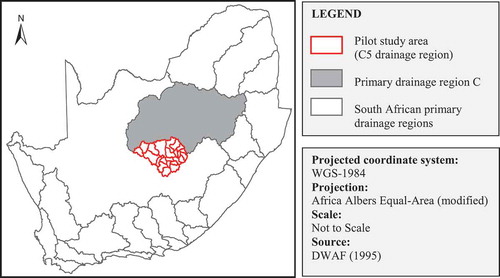
The topography is gentle with slopes of between 2.4 and 5.5% (USGS 2002), while water tends to pond easily, thus influencing the attenuation and translation of floods. The average mean annual precipitation (MAP) for the C5 secondary drainage region is 424 mm, ranging from 275 mm year^-1 in the west to 685 mm year^-1 in the east (Lynch 2004), and rainfall is characterized as highly variable and unpredictable. The rainy season starts in early September and ends in mid-April, with a dry winter. The Modder and Riet rivers are the main river reaches and discharge into the Orange-Vaal River drainage system (Midgley et al. 1994).

4 REVIEW OF CATCHMENT REPSONSE TIME ESTIMATION METHODS

It is necessary to distinguish between the various definitions for time variables and time parameters (T_C, T_L and T_P) before attempting to review the various time parameter estimation methods available.

4.1 Time variables

Time variables can be estimated from the spatial and temporal distributions of rainfall hyetographs and total runoff hydrographs. To estimate these time variables, hydrograph analyses based on the separation of: (a) total runoff hydrographs into direct runoff and baseflow; (b) rainfall hyetographs into initial abstraction, losses and effective rainfall; and (c) the identification of the rainfall−runoff transfer function are required. A convolution process is used to transform the effective rainfall into direct runoff through a synthetic transfer function based on the principle of linear super-positioning, e.g. multiplication, translation and addition (Chow et al. 1988, McCuen 2005).

Effective rainfall hyetographs can be estimated from rainfall hyetographs in one of two different ways, depending on whether observed streamflow data are available or not. In cases where both observed rainfall and streamflow data are available, index methods such as: (i) the Phi-index method, where the index equals the average rainfall intensity above which the effective rainfall volume equals the direct runoff volume, and (ii) the constant-percentage method, where losses are proportional to the rainfall intensity and the effective rainfall volume equals the direct runoff volume, can be used (McCuen 2005). However, in ungauged catchments, the separation of rainfall losses must be based on infiltration methods, which account for infiltration and other losses separately. The SCS runoff curve number method is internationally the most widely used (Chow et al. 1988).

In general, time variables obtained from hyetographs include the peak rainfall intensity, the centroid of effective rainfall and the end time of the rainfall event. Hydrograph-based time variables generally include peak discharges of observed surface runoff, the centroid of direct runoff and the inflection point on the recession limb of a hydrograph (McCuen 2009).

4.2 Time parameters

Most design flood estimation methods require at least one time parameter (T_C, T_L or T_P) as input. In the previous sub-section it was highlighted that time parameters are based on the difference between two time variables, each obtained from a hyetograph and/or hydrograph. In practice, time parameters have multiple conceptual and/or computational definitions, and T_L is sometimes expressed in terms of T_C. Various researchers (e.g. McCuen et al. 1984, Schmidt and Schulze 1984, Simas 1996, McCuen 2005, Jena and Tiwari 2006, Hood et al. 2007, Fang et al. 2008, McCuen 2009) have used the differences between the corresponding values of time variables to define two distinctive time parameters: T_C and T_L. Apart from these two time parameters, other time parameters such as T_P and the hydrograph time base (T_B) are also frequently used.

In the following sub-sections the conceptual and computational definitions of T_C, T_L and T_P are detailed, and the various hydraulic and empirical estimation methods currently in use and their interdependency are reviewed. A total of three hydraulic and 44 empirical time parameter (T_C, T_L and T_P) estimation methods were found in the literature and evaluated. As far as possible, an effort was made to present all the equations in Système International d’Unités (SI) units. Alternatively, the format and units of the equations are retained as published by the original authors.

4.3 Time of concentration

Multiple definitions are used in the literature to define T_C. The most commonly used conceptual, physically-based definition of T_C is the time required for runoff, as a result of effective rainfall, with a uniform spatial and temporal distribution over a catchment, to contribute to the peak discharge at the catchment outlet, in other words, the time required for a “water particle” to travel from the catchment boundary along the longest watercourse to the catchment outlet (Kirpich 1940, McCuen et al. 1984, McCuen 2005, USDA NRCS 2010, SANRAL 2013).

Larson (1965) adopted the concept of time to virtual equilibrium (T_VE), i.e. the time when response equals 97% of the runoff supply, which is also regarded as a practical measure of the actual equilibrium time. The actual equilibrium time is difficult to determine due to the gradual response rate to the input rate. Consequently, T_C defined according to the “water particle” concept would be equivalent to T_VE. However, runoff supply is normally of finite duration, while stream response usually peaks before equilibrium is reached and at a rate lower than runoff supply rate. Pullen (1969) argued that this water particle concept, which underlies the conceptual definition of T_C, is unrealistic, since streamflow responds as an amorphous mass rather than as a collection of drops.

In using such a conceptual definition, the computational definition of T_C is thus the distance travelled along the principal flow path, which is divided into segments of reasonably uniform hydraulic characteristics, divided by the mean flow velocity in each of the segments (McCuen 2009). The current common practice is to divide the principal flow path into segments of overland flow (sheet and/or shallow concentrated flow) and main watercourse or channel flow, after which the travel times in the various segments are computed separately and totalled. Flow length criteria, i.e. overland flow distances (L_O) associated with specific slopes (S_O) are normally used as a limiting variable to quantify overland flow conditions, but a flow retardance factor (i_p), Manning’s overland roughness parameter (n) and overland conveyance factor (ϕ) are also used (Viessman and Lewis 1996, Seybert 2006, USDA NRCS 2010). Seven typical overland slope–distance classes, based on the above-mentioned flow length criteria and as contained in the National Soil Conservation Manual (NSCM) (DAWS 1986), are listed in Table 1. The NSCM criteria are based on the assumption that the steeper the overland slope, the shorter the length of actual overland flow before it transitions into shallow concentrated flow followed by channel flow. McCuen and Spiess (1995) highlighted that the use of such criteria could lead to less accurate designs and proposed that the maximum allowable overland flow path length criteria must rather be estimated as 30.48S_O^0.5n^-1. This criterion is based on the assumption that overland flow dominates where the flow depths are of the same order of magnitude as the surface resistance, i.e. roughness parameters in different slope classes.

Table 1 Overland flow distances associated with different slope classes (DAWS 1986).

Slope class, SO (%)	Distance, LO (m)
0–3	110
3.1–5	95
5.1–10	80
10.1–15	65
15.1–20	50
20.1–25	35
25.1–30	20

The commencement of channel flow is typically defined at a point where a regular, well-defined channel exists with either perennial or intermittent flow, while conveyance factors (default value of 1.3 for natural channels) are also used to provide subjective measures of the hydraulic efficiency, taking both the channel vegetation and degree of channel improvement into consideration (Heggen 2003, Seybert 2006).

The second conceptual definition of T_C relates to the temporal distribution of rainfall and runoff, where T_C is defined as the time between the start of effective rainfall and the resulting peak discharge. The specific computations used to represent T_C based on time variables from hyetographs and hydrographs are discussed in the next paragraph to establish how the different interpretations of observed rainfall−runoff distribution definitions agree with the conceptual T_C definitions in the paragraphs above.

Numerous computational definitions have been proposed for estimating T_C from observed rainfall and runoff data. The following definitions, as illustrated in Fig. 2, are occasionally used to estimate T_C from observed hyetographs and hydrographs (McCuen 2009):

1. the time from the end of effective rainfall to the inflection point on the recession limb of the total runoff hydrograph, i.e. the end of direct runoff; however, this is also the definition used by Clark (1945) to define T_L;

2. the time from the centroid of effective rainfall to the peak discharge of total runoff; however, this is also the definition used by Snyder (1938) to define T_L;

3. the time from the maximum rainfall intensity to the peak discharge; or

4. the time from the start of total runoff (rising limb of hydrograph) to the peak discharge of total runoff.

Fig. 2 Schematic diagram illustrative of the different time parameter definitions and relationships (after Heggen 2003, McCuen 2009).

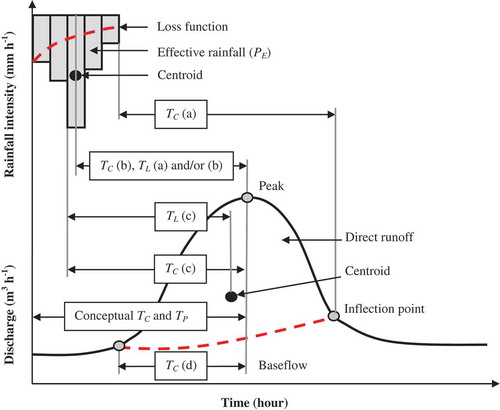
In South Africa, the South African National Roads Agency Limited (SANRAL) recommends the use of T_C definition (d) (SANRAL 2013), but in essence all these definitions are dependent on the conceptual definition of T_C, as described above. It is also important to note that all the definitions listed in (a)–(d) are based on time variables with an associated probability distribution or degree of uncertainty. The “centroid values” denote “average values” and are therefore considered to be more stable time variables representative of the catchment response, especially in larger catchments or where flood volumes are central to the design (McCuen 2009). In contrast to large catchments, the time variables related to peak rainfall intensities and peak discharges are considered to provide the best estimate of the catchment response in smaller catchments where the exact occurrence of the maximum peak discharge is of more importance. McCuen (2009) analysed 41 hyetograph-hydrograph storm event datasets from 20 catchment areas ranging from 1 to 60 ha in the USA. The results from floods estimated using the Rational and/or NRCS TR-55 methods indicated that the T_C based on the conceptual definition and principal flow path characteristics significantly underestimated the temporal distribution of runoff, and that T_C needed to be increased by 56% in order to correctly reflect the timing of runoff from the entire catchment, while the T_C based on T_C definition (b) proved to be the most accurate and was therefore recommended.

The hydraulically-based T_C estimation methods are limited to overland flow, which is derived from uniform flow theory and basic wave mechanics, e.g. the kinematic wave (Henderson and Wooding 1964, Morgali and Linsley 1965, Woolhiser and Liggett 1967), dynamic wave (Su and Fang 2004) and kinematic Darcy-Weisbach (Wong and Chen 1997) approximations. The empirically-based T_C estimation methods are derived from observed meteorological and hydrological data and usually consider the whole catchment, not the sum of sequentially computed reach/segment behaviours. Stepwise multiple regression analyses are generally used to analyse the relationship between the response time and geomorphological, hydrological and meteorological parameters of a catchment. The hydraulic and/or empirical methods commonly used in South Africa to estimate the T_C are discussed in the following paragraphs:

4.3.1 Kerby’s method

This empirical method (equation (1)) is commonly used to estimate T_C both as mixed sheet and/or shallow concentrated overland flow in the upper reaches of small, flat catchments. It was developed by Kerby (1959, cited by Seybert 2006) and is based on the drainage design charts developed by Hathaway (1945, cited by Seybert 2006). Therefore, it is sometimes referred to as the Kerby-Hathaway method. The South African Drainage Manual (SANRAL 2013) also recommends the use of equation (1) for overland flow in South Africa. McCuen et al. (1984) highlighted that this method was developed and calibrated for catchments in the USA with areas of less than 4 ha, average slopes of less than 1% and Manning’s roughness parameters (n) varying between 0.02 and 0.8. In addition, the length of the flow path is a straight-line distance from the most distant point on the catchment boundary to the start of a fingertip tributary (well-defined watercourse) and is measured parallel to the slope. The flow path length must also be limited to ±100 m.

(1)

where T_C1 is overland time of concentration (min), L_O is length of overland flow path (m), limited to 100 m, n is Manning’s roughness parameter for overland flow, and S_O is the average overland slope (m m^-1).

4.3.2 SCS method

This empirical method (equation (2)) is commonly used to estimate T_C as mixed sheet and/or concentrated overland flow in the upper reaches of a catchment. The USDA SCS (later NRCS) developed this method in 1962 for homogeneous, agricultural catchment areas of up to 8 km², with mixed overland flow conditions dominating (Reich 1962). The calibration of equation (2) was based on T_C definition (c) (see Section 4.3) and a T_C:T_L proportionality ratio of 1.417 (McCuen 2009). However, McCuen et al. (1984) showed that equation (2) provides accurate T_C estimates for catchment areas up to 16 km².

(2)

where T_C2 is overland time of concentration (min), CN is the runoff curve number, L_O is length of overland flow path (m), and S is average catchment slope (m m^-1).

4.3.3 NRCS velocity method

This hydraulic method is commonly used to estimate T_C both as shallow concentrated overland and/or channel flow (Seybert 2006). Either equation (3a) or (3b) can be used to express the T_C for concentrated overland or channel flow. In the case of main watercourse/channel flow, this method is referred to as the NRCS segmental method, which divides the flow path into segments of reasonably uniform hydraulic characteristics. Separate travel time calculations are performed for each segment based on either equation (3a) or (3b), while the total T_C is computed using equation (3c) (USDA NRCS 2010):

(3a)

(3b)

(3c)

where T_C3 is overland/channel flow time of concentration computed using the NRCS method (min), T_C3(i) is overland/channel flow time of concentration of segment i (min), k_s is Chézy’s roughness parameter (m), L_O,CH is length of flow path, either overland or channel flow (m), n is Manning’s roughness parameter, R is hydraulic radius which equals the flow depth (m), and S_O,CH is average overland or channel slope (m m^-1).

4.3.4 USBR method

Equation (4) was proposed by the USBR (1973) to be used as a standard empirical method to estimate the T_C in hydrological designs, especially culvert designs based on the California Culvert Practice (CPP 1955, cited by Li and Chibber 2008). However, equation (4) is essentially a modified version of the Kirpich method (Kirpich 1940) and is recommended by SANRAL (2013) for use in South Africa for defined, natural watercourses/channels. It is also used in conjunction with equation (1), which estimates overland flow time, to estimate the total travel time (overland plus channel flow) for deterministic design flood estimation methods in South Africa. Van der Spuy and Rademeyer (2010) highlighted that equation (4) tends to result in estimates that are either too high or too low, and recommend the use of a correction factor (τ), as shown in equation (4a) and listed in Table 2.

(4)

(4a)

Table 2 Correction factors (τ) for T_C (Van der Spuy and Rademeyer 2010).

Area, A (km^2)	Correction factor, τ
<1	2
1–100	2−0.5 logA
100–5 000	1
5 000–100 000	2.42−0.385 logA
>100 000	0.5

where T_C4,4a is channel flow time of concentration (h), L_CH is length of longest watercourse (km), S_CH is average main watercourse slope (m m^-1), and τ is a correction factor.

In addition to the above-listed methods used in South Africa, Table A1 in the Appendix contains a detailed description of a selection of other T_C estimation methods used internationally. It is important to note that most of the T_C methods discussed above and listed in Table A1 are based on an empirical relationship between physiographic parameters and a characteristic response time, usually T_P, which is then interpreted as T_C.

4.4 Lag time

Conceptually, T_L is generally defined as the time between the centroid of effective rainfall and the peak discharge of the resultant direct runoff hydrograph, which is the same as the T_C definition (b) as shown in Fig. 2. Computationally, T_L can be estimated as a weighted T_C value when, for a given storm, the catchment is divided into sub-areas and the travel times from the centroid of each sub-area to the catchment outlet are established by the relationship expressed in equation (5). This relationship is also illustrated in Fig. 3 (USDA NRCS 2010).

(5)

Fig. 3 Conceptual travel time from the centroid of each sub-area to the catchment outlet (USDA NRCS 2010).

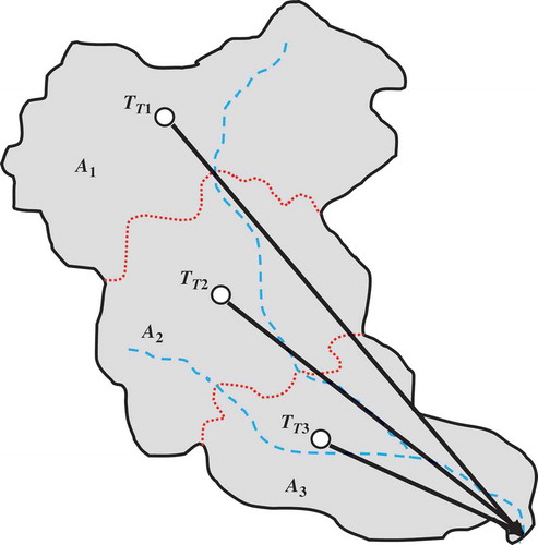
where T_L is lag time (h), A_i is incremental catchment area/sub-area (km²), Q_i is incremental runoff from A_i (mm), and T_Ti is travel time from the centroid of A_i to catchment outlet (h).

In flood hydrology, T_L is normally not estimated using equation (5). Instead, either empirical or analytical methods are used to analyse the relationship between the response time and meteorological and geomorphological parameters of a catchment. In the following paragraph, the meteorological parameters, as defined by different interpretations of observed rainfall−runoff distribution definitions are explored.

Scientific literature often fails to clearly define and distinguish between T_C and T_L, especially when observed data (hyetographs and hydrographs) are used to estimate these time parameters. The differences between time variables from various points on hyetographs to various points on the resultant hydrographs are sometimes misinterpreted as T_C. The following definitions, as illustrated in Fig. 2, are occasionally used to estimate T_L as a time parameter from observed hyetographs and hydrographs (Heggen 2003):

1. the time from the centroid of effective rainfall to the time of the peak discharge of direct runoff;

2. the time from the centroid of effective rainfall to the time of the peak discharge of total runoff; or

3. the time from the centroid of effective rainfall to the centroid of direct runoff.

As in the case of T_C, T_L is also based on uncertain, inconsistently defined time variables. However, T_L definitions (a)–(c) listed above use centroid values and are therefore considered likely to be more stable time variables that are representative of the catchment response in large catchments. Pullen (1969) also highlighted that T_L is preferred as a measure of catchment response time, especially due to the incorporation of storm duration in these definitions. Definitions (a)–(c) are generally used or defined as T_L (Simas 1996, Hood et al. 2007, Folmar and Miller 2008, Pavlovic and Moglen 2008), although T_L definition (b) is also sometimes used to define T_C.

Dingman (2002, cited by Hood et al. 2007) recommended the use of equation (6) to estimate the centroid values of hyetographs or hydrographs:

(6)

where C_P,Q is the centroid value of rainfall or runoff (mm or m³ s^-1), t_i is time for period i (h), N is sample size, and X_i is rainfall or runoff for period i (mm or m³ s^-1).

Owing to the difficulty in estimating the centroid of hyetographs and hydrographs, other T_L estimation techniques have been proposed. Instead of using T_L as an input for design flood estimation methods, it is rather used as input to the computation of T_C. In using T_L definition (c), T_C and T_L are normally related by T_C = 1.417T_L (McCuen 2009). In T_L definitions (a) and (b), the proportionality factor increases to 1.67 (McCuen 2009). However, Schultz (1964) established that for small catchments in Lesotho and South Africa, T_L ≈ T_C, which conflicts with these proposed proportionality factors. The empirical methods commonly used in South Africa to estimate T_L are discussed in the following paragraphs.

4.4.1 HRU method

This method was developed by the HRU (Pullen 1969) in conjunction with the development of synthetic unit hydrographs (SUHs) for South Africa (HRU 1972). The lack of continuously recorded rainfall data for medium to large catchments in South Africa forced Pullen (1969) to develop an indirect method to estimate T_L using only observed streamflow data from 96 catchment areas ranging from 21 to 22 163 km². Pullen (1969) assumed that the onset of effective rainfall coincides with the start of direct runoff, and that the T_P could be used to describe the time lapse between this mutual starting point and the resulting peak discharge. In essence, it was acknowledged that direct runoff is unable to recede before the end of effective rainfall; therefore the T_P was regarded as the upper limit storm duration during the implementation of the unit hydrograph theory using the S-curve technique. In other words, a hydrograph of 25 mm of direct runoff was initially assumed to be a T_P-hour unit hydrograph. However, due to non-uniform temporal and spatial runoff distributions, possible inaccuracies in streamflow measurements and non-linearities in catchment response characteristics, the S-curves fluctuated about the equilibrium discharge amplitude. Therefore, the analysis was repeated using descending time intervals of 1 h until the fluctuations of the S-curve ceiling value diminished to within a prescribed 5% range. After the verification of the effective rainfall durations, all the hydrographs of 25 mm of direct runoff were converted to unit hydrographs of relevant duration. To facilitate the comparison of these unit hydrographs derived from different events in a given catchment, all the unit hydrographs for a given record were then converted by the S-curve technique to unit hydrographs of standard duration (Pullen 1969).

Thereafter, the centroid of each unit hydrograph was determined by simple numerical integration of the unit hydrograph from time zero. The T_L values were then simply estimated as the time lapse between the centroid of effective rainfall and the centroid of a unit hydrograph (Pullen 1969). The catchment-index (L_HL_CS_CH^-0.5), as proposed by the US Army Corps of Engineers (USACE) (Linsley et al. 1988) was used to estimate the delay of runoff from the catchments. The T_L values (criterion variables) were plotted against the catchment indices (predictor variables) on logarithmic scales. Least-square regression analyses were then used to derive a family of T_L equations applicable to each of the nine homogeneous veld-type regions with representative SUHs in South Africa, as expressed by equation (7). The regionalization scheme of the veld-type regions took into consideration catchment characteristics, e.g. topography, soil type, vegetation and rainfall, which are most likely to influence catchment storage and therefore T_L.

(7)

where T_L1 is lag time (h), C_T is regional storage coefficient (Table 3), L_C is centroid distance (km), L_H is hydraulic length of catchment (km), and S_CH is average main watercourse slope (m m^-1).

Table 3 Generalized regional storage coefficients (HRU 1972).

Veld region	Veld-type description	CT1
1	Coastal tropical forest	0.99
2	Schlerophyllous bush	0.62
3	Mountain sourveld	0.35
4	Grassland of interior plateau	0.32
5	Highland sourveld and Dohne sourveld	0.21
5A	Zone 5, soils weakly developed	0.53
6	Karoo	0.19
7	False Karoo	0.19
8	Bushveld	0.19
9	Tall sourveld	0.13

4.4.2 SCS lag method

In sub-section 4.3.2 it was highlighted that this method was developed by the USDA SCS in 1962 (Reich 1962) to estimate T_C where mixed overland flow conditions in catchment areas of up to 8 km² exist. However, using the relationship T_L = 0.6T_C, equation (8) can also be used to estimate T_L in catchment areas of up to 16 km² (McCuen 2005).

(8)

where T_L2 is lag time (h), CN is the runoff curve number, L_H is the hydraulic length of the catchment (km), and S is the average catchment slope (m m^-1).

4.4.3 Schmidt-Schulze (SCS-SA) method

Schmidt and Schulze (1984) estimated T_L from observed rainfall and flow data in 12 agricultural catchments in South Africa and the USA, with catchment areas smaller than 3.5 km², by using three different methods to develop equation (9). This equation is used in preference to the original SCS lag method (equation (8)) in South Africa, especially when stormflow response includes both surface and subsurface runoff, as frequently encountered in areas of high MAP or on natural catchments with good land cover (Schulze et al. 1992).

(9)

where T_L3 is lag time (h), A is catchment area (km²), i₃₀ is 2-year return period 30-min rainfall intensity (mm h^-1), MAP is mean annual precipitation (mm), and S is average catchment slope (%).

The three different methods used to develop equation (9) are based on the following approach (Schmidt and Schulze 1984):

Initially, the relationship between peak discharge and volume was investigated by regressing linear peak discharge distributions (single triangular hydrographs) against the corresponding runoff volume obtained from observed runoff events to determine the magnitude and intra-catchment variability of T_L. Thereafter, the incremental triangular hydrographs were convoluted with observed effective rainfall to form compound hydrographs representative of the peak discharge and temporal runoff distribution of observed hydrographs. Lastly, the average time response between effective rainfall and direct runoff was measured in each catchment to determine an index of catchment lag time. It was concluded that intra-catchment T_L estimates in ungauged catchments can be improved by incorporating indices of climate and regional rainfall characteristics into an empirical lag equation. The 2-year return period 30-min rainfall intensity proved to be the dominant rainfall parameter that influences intra-catchment variations in T_L estimates (Schmidt and Schulze 1984).

In addition to the above-listed methods used in South Africa, Table A2 in the Appendix contains a detailed description of a selection of other T_L estimation methods used internationally.

4.5 Time to peak

The T_P, which is used in many hydrological applications, can be defined as the time from the start of effective rainfall to the peak discharge in a single-peaked hydrograph (McCuen et al. 1984, USDA SCS 1985, Linsley et al. 1988, Seybert 2006). However, this is also the conceptual definition used for T_C (see Fig. 2). The T_P is also sometimes defined as the time interval between the centroid of effective rainfall and the peak discharge of direct runoff (Heggen 2003); however, this is also one of the definitions used to quantify T_C and T_L using T_C definition (b) and T_L definition (c), respectively. According to Ramser (1927), T_P is regarded to be synonymous with T_C and both these time parameters are reasonably constant for a specific catchment. In contrast, Bell and Kar (1969) concluded that these time parameters are far from being constant; in fact, they may deviate between 40% and 200% from the median value.

The SCS-Mockus method (equation (10)) is the only empirical method occasionally used in South Africa to estimate T_P based on the SUH research conducted by Snyder (1938), while Mockus (1957, cited by Viessman et al. 1989) developed the SCS SUHs from dimensionless unit hydrographs, as obtained from a large number of natural hydrographs in various catchments with variable sizes and geographical locations. Only the T_P and Q_P values are required to approximate the associated SUHs, while the T_P is expressed as a function of the storm duration and T_L. Equation (10) is based on T_L definition (c), while it also assumes that the effective rainfall is constant with the centroid at P_D/2.

(10)

where T_P1 is time to peak (h), P_D is storm duration (h), and T_L is lag time based on equation (8) (h).

Table A3 in the Appendix contains a detailed description of a selection of other T_P estimation methods used internationally.

5 METHODOLOGY

To evaluate and compare the consistency of a selection of time parameter estimation methods in the pilot study area, the following steps were initially followed: (a) estimation of climatological variables (driving mechanisms), and (b) estimation of catchment variables and parameters (which act as buffers and/or responses to the drivers). The steps involved in (a) and (b) are discussed first, followed by the evaluation and comparison of the catchment response time estimation methods.

It is acknowledged that the empirical methods selected for comparison purposes are applied outside their bounds in terms of both areal extent and their original developmental regions. This is purposely done for comparison purposes, as well as to reflect the engineering practitioner’s dilemma in doing so, especially due to the absence of locally developed and verified methods at this catchment scale in South Africa.

5.1 Climatological variables

The average 2-year, 24-h rainfall depths, as required by the NRCS kinematic wave method (equation (A2)) of each catchment under consideration were obtained from Gericke and Du Plessis (2011), who applied the isohyetal method at a 25-mm interval using the Interpolation and Reclass toolset of the Spatial Analyst Tools toolbox in ArcGIS^TM 9.3, in conjunction with the design point rainfall depths as contained in the Regional L-Moment Algorithm SAWS n-day design point rainfall database (RLMA-SAWS) (after Smithers and Schulze 2000). The critical storm durations as required to estimate T_P were obtained from Gericke (2010) and Gericke and Du Plessis (2013), who applied the SUH method in all the catchments under consideration. In each case, user-defined critical storm durations based on a trial-and-error approach were used to establish the critical storm duration which results in the highest peak discharge.

5.2 Catchment geomorphology

All the relevant geographical information system (GIS) and catchment related data were obtained from the Department of Water Affairs (DWA, Directorate: Spatial and Land Information Management), which is responsible for the acquisition, processing and digitising of the data. The specific GIS data feature classes (lines, points and polygons) applicable to the study area and individual sub-catchments were extracted and created from the original GIS datasets. The data extraction was followed by data projection and transformation, editing of attribute tables and recalculation of catchment geometry (areas, perimeters, widths and hydraulic lengths). These geographical input datasets were transformed to a projected coordinate system using the Africa Albers Equal-Area projected coordinate system with modification (ESRI 2006).

The average slope of each catchment under consideration was based on a projected and transformed version of the Shuttle Radar Topography Mission (SRTM) digital elevation model (DEM) data for Southern Africa at 90-m resolution (USGS 2002). The catchment centroids were determined by making use of the Mean Center tool in the Measuring Geographic Distributions toolset contained in the Spatial Statistics Tools toolbox of ArcGIS^TM 9.3. Thereafter, all the above-mentioned catchment information was used to estimate the catchment shape parameters, circularity and elongation ratios, all of which may have an influence on the catchment response time.

5.3 Catchment variables

Both the weighted runoff curve numbers (CN), as required by equations (2), (8) and (A32), and weighted runoff coefficients, as required by equation (A4), were obtained from the analyses performed by Gericke and Du Plessis (2013). The catchment storage coefficients, as applicable to the HRU T_L estimation method (equation (7)), were obtained from Gericke (2010), while the catchment storage coefficients applicable to the T_L estimation methods of Snyder (1938) (equation (A16)), USACE (1958) (equation (A18)) and Bell and Kar (1969) (equation (A21)), were based on the default values as proposed by the original authors.

5.4 Channel geomorphology

The main watercourses in each catchment were firstly manually identified in ArcMap. Thereafter, a new shapefile containing polyline feature classes representative of the identified main watercourse was created by making use of the Trace tool in the Editor Toolbar using the polyline feature classes of the 20-m interval contour shapefile as the specified offset or point of intersection, to result in chainage distances between two consecutive contours. The average slope of each main watercourse was estimated using the 10–85 method (Alexander 2001, SANRAL 2013). The channel conveyance factors, as required by the Espey-Altman T_P estimation method (equation (A37)), were based on the default values proposed by Heggen (2003) for natural channels. However, in practice, detailed surveys and mapping are required to establish these conveyance factors more accurately.

5.5 Estimation of catchment response time

The current common practice of dividing the principal flow path into segments of overland flow and main watercourse or channel flow to estimate the total travel time, was acknowledged. However, since this study focuses on medium to large catchments in which the main watercourse, i.e. channel flow, presumably dominates, the overland flow T_C estimation methods were not evaluated for specific catchments, but were estimated for the seven different NSCM slope–distance classes (DAWS 1986), as listed in Table 1.

Six overland flow T_C estimation methods, equations (1), (2) and (A2)–(A4), (A6) from Table A1, with similar input variables were evaluated by taking cognisance of the maximum allowable overland flow path length criteria as proposed by McCuen and Spiess (1995). In addition, five different categories defined by specific, interrelated overland flow retardance (i_p), Manning’s roughness (n) and overland conveyance (ϕ) factors were also considered. The five different categories (i_p, n and ϕ) were based on the work done by Viessman and Lewis (1996), who plotted the ϕ values as a function of Manning’s n and i_p values. Typical ϕ values ranged from 0.6 (n = 0.02; i_p = 80%), 0.8 (n = 0.06; i_p = 50%), 1.0 (n = 0.09; i_p = 30%), 1.2 (n = 0.13; i_p = 20%) to 1.3 (n = 0.15; i_p = 10%). By considering all these factors, it was argued that both the consistency and sensitivity of the methods under consideration in this flow regime could be evaluated.

A selection of seven T_C (equations (4), (4a) and equations (A8–A10, A13, A15b) from Table A1), 15 T_L (equations (7), (8) and equations (A16–A18, A21, A23–A25, A27–A29, A31–A33) from Table A2) and five T_P (equation (10) and equations (A34–35, A37–A38) from Table A3) estimation methods were also applied to each sub-catchment under consideration using an automated spreadsheet developed in Microsoft Excel 2007. The selection of the methods was based on the similarity of catchment input variables required, e.g. A, CN, C_T, i_p, L_C, L_CH, L_H, S, S_CH and/or ϕ_CH (see Table 4).

Table 4 General catchment information. P₂: 2-year return period 24-h rainfall depth (mm); P_D: unit hydrograph critical storm duration (h); A: area (km²); A_C: circle-area (km²) with perimeter = catchment perimeter; P: perimeter (km); W: width (km); L_C: centroid distance (km); L_H: hydraulic length of catchment (km); L_M: max. length parallel to principal drainage line (km); L_S: max. straight-line catchment length (km); S: average catchment slope (m m^-1); F_S1: shape parameter; R_C1: circularity ratio; R_E: elongation ratio; i_p: imperviousness/urbanization factor (%); CN: weighted runoff curve number; C: weighted rational runoff coefficient; C_SDF: regional SDF runoff coefficient; C_T1: HRU regional storage coefficient; C_T2: Snyder’s storage coefficient; C_T3: USACE storage coefficient ; C_T4: Bell-Kar storage coefficient; L_CH: length of channel flow path (km); S_CH: average slope of channel flow path (m m^-1); ϕ_CH: channel conveyance factor; τ: USBR channel flow correction factor.

Catchment descriptors	C5R001	C5R002	C5R003	C5R004	C5R005	C5H003	C5H012	C5H015	C5H016	C5H018	C5H022	C5H054
Climatological variables
P2 (mm)	50	48	54	54	54	54	48	54	50	52	54	54
PD (h)	10	17	7	16	2	7	8	12	40	34	1.5	7
Catchment geomorphology
A (km^2)	922	10 260	937	6 331	116	1 650	2 366	6 009	33 277	17 360	38	688
AC (km^2)	2063	22 269	1 743	13 377	168	2 903	4 210	10 029	77 208	50 930	134	1 696
P (km)	161	529	148	410	46	191	230	355	985	800	41	146
W (km)	17	98	23	66	10	32	47	66	125	64	11	12
LC (km)	53	97	31	113	8	41	48	101	237	233	4	33
LH (km)	86	202	54	187	16	71	87	167	431	375	8	68
LM (km)	55	136	42	141	14	54	60	125	301	272	7	55
LS (km)	49	132	43	118	14	54	59	118	250	225	7	51
S (m m^-1)	0.03054	0.04369	0.05044	0.04186	0.05501	0.05044	0.04771	0.04186	0.03598	0.03211	0.05501	0.03659
FS1	2.6	1.7	2.0	2.2	1.7	1.8	1.5	2.3	1.9	2.9	1.3	3.8
RC1	1.5	1.5	1.4	1.5	1.2	1.3	1.3	1.3	1.5	1.7	1.9	1.6
RE	0.6	0.8	0.8	0.6	0.9	0.8	0.9	0.7	0.7	0.5	1.0	0.5
Catchment variables
ip (%)	5	8	5	5	8	5	10	5	5	5	8	5
CN	78	77.6	76.3	74.4	76.2	76.3	78.3	74.4	69.8	69.8	76.2	77.6
C (T = 2-year)	0.368	0.365	0.358	0.319	0.491	0.358	0.417	0.319	0.283	0.283	0.491	0.283
CSDF (T = 100-year)	0.600	0.600	0.600	0.600	0.600	0.600	0.600	0.600	0.600	0.600	0.600	0.600
CT1	0.268	0.221	0.320	0.317	0.320	0.320	0.194	0.317	0.246	0.246	0.320	0.291
CT2	1.350	1.350	1.500	1.600	1.500	1.500	1.350	1.600	1.600	1.600	1.500	1.500
CT3	0.249	0.268	0.278	0.266	0.327	0.278	0.273	0.266	0.254	0.254	0.327	0.259
CT4	0.05	0.05	0.05	0.05	0.05	0.05	0.05	0.05	0.05	0.05	0.05	0.05
Channel geomorphology
LCH (km)	86	202	54	187	16	71	87	167	431	375	8	68
SCH (m m^-1)	0.00229	0.00133	0.00273	0.00131	0.00895	0.00232	0.00269	0.00139	0.00078	0.00079	0.01687	0.00261
ϕCH	1.3	1.3	1.3	1.3	1.3	1.3	1.3	1.3	1.3	1.3	1.3	1.3
τ	1	0.876	1	0.956	1	1	1	0.965	0.679	0.788	1.210	1

5.6 Comparison of catchment response time estimation results

Taking into consideration that this study only attempts to provide preliminary insight into the consistency of the various time parameter estimation methods in South Africa, as well to provide recommendations for improving catchment response time estimation in medium to large catchments, the comparison of the methods is intended to highlight only biases and inconsistencies in the methods. Therefore, in the absence of observed time parameters at this stage of the study, the selected methods were compared to the generally “recommended methods” currently used in South Africa, e.g. overland flow T_C (Kerby’s method, equation (1)), channel flow T_C (USBR method, equation (4)), T_L (HRU method, equation (7)) and T_P (SCS-Mockus method, equation (10)). The mean error (difference in the average of the “recommended value” and estimated values in different classes/categories/sub-catchments) was used as a measure of actual bias. However, a method’s mean error could be dominated by errors in the large time parameter values; subsequently a standardized bias statistic (equation (11); McCuen et al. 1984) was also introduced. The standard error of the estimate was also used to provide another measure of consistency:

(11)

where B_S is the standardized bias statistic (%), T_X is the time parameter estimate based on the recommended methods (min or h), T_Y is the time parameter estimate using other selected methods (min or h), and z is the number of slope–distance categories or sub-catchments.

To appreciate the significance of the inconsistencies introduced by using the various time parameter estimation methods, the results were translated to design peak discharges. In order to do so, the 100-year design rainfall depths associated with the critical storm duration in each of the 12 sub-catchments (Gericke and Du Plessis 2011), along with the catchment areas and regional runoff coefficients (Table 4), were substituted into the Standard Design Flood (SDF) method to estimate design peak discharges. The SDF method (equation (12)) is a regionally calibrated version of the Rational method, and is deterministic-probabilistic in nature and applicable to catchment areas of up to 40 000 km² (Alexander 2002, Gericke and Du Plessis 2012, SANRAL 2013).

(12)

where Q_T is design peak discharge (m³ s^-1), A is catchment area (km²), C₂ is a 2-year return period runoff coefficient (15% for the pilot study area), C₁₀₀ is a 100-year return period runoff coefficient (60% for the pilot study area), I_T is average design rainfall intensity (mm h^-1), and Y_T is a log-normal standard variate (return period factor).

6 RESULTS

6.1 Review of catchment response time estimation methods

The use of time parameters based on either hydraulic or empirical estimation methods was evident from the literature review conducted. It was confirmed that none of these hydraulic and empirical methods are highly accurate or consistent in providing the true value of the time parameters, especially when applied outside their original developmental regions. In addition, many of these methods/equations proved to be in disparate forms and are presented without explicit unit specifications or suggested values for constants. For example, with the migration between dimensional systems, what seems to be a Manning’s roughness coefficient (n) value, is in fact a special-case roughness coefficient. Heggen (2003), who summarized more than 80 T_C, T_L and T_P estimation methods from the literature, confirmed these findings.

6.2 General catchment information

The general catchment information (e.g. climatological variables, catchment geomorphology, catchment variables and channel geomorphology) applicable to each of the 12 sub-catchments in the pilot study area is listed in Table 4. The influence of each variable or parameter listed in Table 4 will be highlighted where applicable in the subsequent sub-sections which focus on the time parameter estimation results.

6.3 Comparison of catchment response time estimation results

The results from the application of the time parameter estimation methods applicable to the overland flow and predominant channel flow regimes, as well as a possible combination thereof, are listed and discussed in the following sections.

6.3.1 Catchment time of concentration

The five methods used to estimate the T_C in the overland flow regime, relative to the T_C estimated using the Kerby equation (equation (1)), showed different biases when compared to this recommended method in each of the five different flow retardance categories and associated slope–distance classes. As expected, all the T_C estimates decreased with an increase in the average overland slope, while T_C gradually increases with an increase in the flow retardance factors (i_p, n and ϕ). Two of the methods (SCS and Miller) constantly underestimated T_C, except in Categories 1 and 2 for average overland slopes <0.05 m m^-1. The other three methods (NRCS, FAA and Espey-Winslow) overestimated T_C in all cases, with the poorest results demonstrated by the Espey-Winslow method (equation (A6)). These poor estimates could be ascribed to the use of default conveyance (ϕ) factors that might not be representative, since the latter method is the only method using ϕ as a primary input parameter. Significant biases, e.g. over- or under-estimations, also highlighted the presence of systematic errors.

Table 5 contains the overall average consistency measures based on the above-mentioned comparisons. In each case, the bias is summarized using equation (11), while the mean error represents the average difference between the mean recommended T_C and the mean estimated T_C values as established considering each of the afore-mentioned classes and categories.

Table 5 Consistency measures for the test of overland flow T_C estimation methods compared to the “recommended method” (equation (1)).

Method	Consistency measure
	Mean recommended TC (min)	Mean estimated TC (min)	Standard bias statistic (%)	Mean error (min)	Maximum error (min)	Standard error (min)
SCS, equation (2)	5.3	3.8	−30.6	−1.5	4.7	1.8
NRCS, equation (A2)	5.3	8.4	32.7	3.1	−17.6	0.5
Miller, equation (A3)	5.3	2.4	−57.3	−2.9	−6.0	1.1
FAA, equation (A4)	5.3	9.7	97.4	4.4	14.0	1.7
Espey-Winslow, equation (A6)	5.3	31.1	469.2	25.8	−81.5	1.8

On average, the SCS and NRCS kinematic wave methods provided relatively small biases (<35%), with mean errors of ≤3.1 min. Both the standardized bias (469.2%) and mean error (26 min) of the Espey-Winslow method (equation (A6)) were large compared to the other methods. The SCS method resulted in the smallest maximum absolute error of 5 min, while the Espey-Winslow method had a maximum absolute error of 82 min. The standard deviation of the errors provides another measure of consistency; only the NRCS kinematic wave method resulted in a standard error of <1 min.

Table 6 contains the NSCM flow length criteria (cf. Table 1, DAWS 1986) and the maximum allowable overland flow path length results based on the McCuen and Spiess (1995) criteria. The results differed significantly and could be ascribed to the fact that McCuen and Spiess (1995) associated the occurrence of overland flow with flow depths that are of the same order of magnitude as the surface resistance, while the NSCM criteria are based on the assumption that the steeper the overland slope, the shorter the length of actual overland flow before it transitions to shallow concentrated flow followed by channel flow. In applying the McCuen-Spiess criteria, the shorter overland flow path lengths were associated with flatter slopes and higher roughness parameter values. Although, the latter association with higher roughness parameter values seems to be logical in such a case, the proposed relationship of 30.48S_O^0.5n^-1 occasionally resulted in overland lengths of up to 835 m. It is important to note that most of the overland flow equations are assumed to be applicable up to ±100 m (USDA SCS 1985), which almost coincides with the maximum overland flow length of 110 m as proposed by the DAWS (1986).

Table 6 Comparison of maximum overland flow length criteria.

Average overland slope class (SO, m m^-1)		0.03	0.05	0.10	0.15	0.20	0.25	0.30
NSCM flow length criteria (LO, m)		110	95	80	65	50	35	20
McCuen-Spiess flow length criteria (LO, m)
Roughness parameters	0.02	264	341	482	590	682	762	835
	0.06	88	114	161	197	227	254	278
	0.09	59	76	107	131	151	169	185
	0.13	41	52	74	91	105	117	128
	0.15	35	45	64	79	91	102	111

The six methods used to estimate T_C, under predominant channel flow conditions, relative to the T_C estimated using the USBR equation (equation (4)), showed different biases when compared to this recommended method in each of the 12 sub-catchments of the study area, as illustrated in Fig. 4. As expected, all the T_C estimates increased with an increase in catchment size, although in the areal range between 922 km² (C5R001) and 937 km² (C5R003), the T_C estimates decreased despite the increase in area. This is most likely due to the steeper average catchment slope and shorter channel flow path characterizing the larger catchment area.

Fig. 4 T_C estimation results.

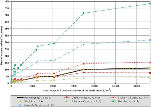
Table 7 contains the overall average consistency measures based on the comparisons depicted in Fig. 4. The Kirpich method (equation (A9)) showed the smallest bias and a mean error of zero; this was expected since equation (4) is essentially a modified version of the Kirpich method. The USBR (equation (4a), with correction factors) and Johnstone-Cross (equation (A10)) methods also provided relatively small negative biases (<–50%), but their associated negative mean errors were 5.5 h and 21.7 h, respectively. Both the standardized biases (315% and 538%) and mean errors (87 h and 172 h) of the Colorado-Sabol (equation (A15b)) and Sheridan (equation (13)) methods, respectively, were much larger when compared to the other methods.

Table 7 Consistency measures for the test of channel flow T_C estimation methods compared to the “recommended method”, equation (4).

Method	Consistency measure
	Mean recommended TC (h)	Mean estimated TC (h)	Standard bias statistic (%)	Mean error (h)	Maximum error (h)	Standard error (h)
USBR correction, equation (4a)	37.3	31.8	−4.4	−5.5	−35.7	6.4
Bransby-Williams, equation (A8)	37.3	54.9	57.8	17.6	43.5	1.4
Kirpich, equation (A9)	37.3	37.3	0.0	0.0	−0.1	0.0
Johnstone-Cross, equation (A10)	37.3	15.6	−5.0	−21.7	−71.0	3.0
Sheridan, equation (A13)	37.3	209.6	537.9	172.3	472.0	1.8
Colorado-Sabol, equation (A15b)	37.3	124.0	315.4	86.7	205.4	3.5

Most of the methods showed inconsistency in at least one of the 12 sub-catchments. The Kirpich method (equation (A9)) resulted in the smallest maxi-mum absolute error of –0.1 h in three sub-catchments, while Sheridan’s method had a maximum absolute error of 472 h in catchment C5H016. Typically, the high errors associated with Sheridan’s method could be ascribed to the fact that only one predictor variable (e.g. only main watercourse length) was used in attempt to accurately reflect the catchment response time, i.e. the criterion variable.

In translating these mean errors of between –15% and 462% to design peak discharges using the SDF method, their significance is truly appreciated. The underestimation of T_C is associated with the overestimation of peak discharges or vice versa, viz. the overestimation of T_C results in underestimated peak discharges. Typically, the T_C underestimations ranged between 20% and 65%, which resulted in peak discharge overestimations of between 30% and 175%, while T_C overestimations of up to 700% resulted in maximum peak discharge underestimations of 90%.

6.3.2 Catchment lag time

Figure 5 illustrates the results of the 14 methods used to estimate T_L relative to the T_L estimated using the HRU equation (equation (7)) in each of the 12 sub-catchments of the pilot study area. It is interesting to note that, as in the case of the T_C estimates, most of the methods based on (L_CHS_CH^-1)^X ratios as primary input, resulted in T_L estimates that decreased despite the increase in area. This was quite evident in catchments with a decreasing channel flow path length (L_CH) and increasing average channel slope (S_CH) associated with an increase in catchment size. In addition, these lower L_CH values contributed to shape parameter (F_S1, Table 4) differences of more than 0.5. This also confirms that catchment geomorphology and catchment variables play a key role in catchment response times.

Fig. 5 T_L estimation results.

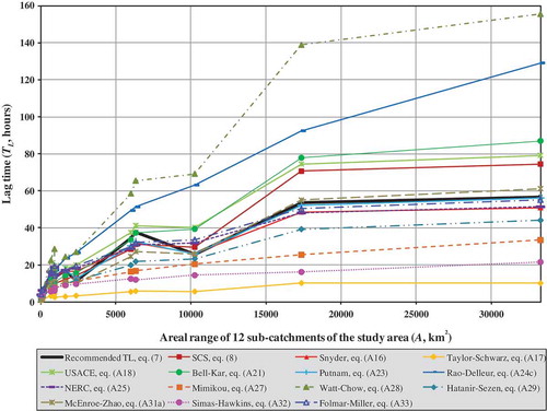
Table 8 contains the overall average consistency measures based on the comparisons depicted in Fig. 5.

Table 8 Consistency measures for the test of T_L estimation methods compared to the “recommended method”, equation (7).

Method	Consistency measure
	Mean recommended TL (h)	Mean estimated TL (h)	Standard bias statistic (%)	Mean error (h)	Maximum error (h)	Standard error (h)
SCS, equation (8)	23.9	25.6	–0.5	1.7	17.8	5.0
Snyder, equation (A16)	23.9	23.1	12.1	–0.8	–6.0	2.2
Taylor-Schwarz, equation (A17)	23.9	4.6	–78.3	–19.3	–46.6	4.2
USACE, equation (A18)	23.9	30.6	25.4	6.8	22.5	3.7
Bell-Kar, equation (A21)	23.9	29.1	5.2	5.2	30.3	4.7
Putnam, equation (A23)	23.9	23.7	4.4	–0.2	–5.2	2.3
Rao-Delleur, equation (A24c)	23.9	41.1	56.1	17.2	72.4	6.1
NERC, equation (A25)	23.9	23.8	15.0	–0.1	–7.0	4.0
Mimikou, equation (A27)	23.9	13.3	–38.3	–10.6	–28.1	6.1
Watt-Chow, equation (A28)	23.9	51.2	82.7	27.4	98.8	4.8
Haktanir-Sezen, equation (A29)	23.9	16.9	–29.8	–7.0	–15.9	4.4
McEnroe-Zhao, equation (A31a)	23.9	20.7	–24.8	–3.2	–10.5	4.2
Simas-Hawkins, equation (A32)	23.9	10.2	–40.0	–13.7	–37.4	7.3
Folmar-Miller, equation (A33)	23.9	24.9	20.2	1.0	8.2	4.3

The 14 T_L estimation methods (Table 8) proved to be less biased than the T_C estimation methods when compared to the recommended method (HRU, equation (7)), with standardized biases ranging from –78.3% to 82.7%. Five methods (e.g. SCS, Snyder, Putnam, NERC and Folmar-Miller) with similar predictor variables (e.g. L_H and S_CH) as used in the recommended method showed the smallest biases (<20%) and mean errors (<2 h). The USACE method (equation (A18)), which is essentially identical to the recommended method, apart from the different regional storage coefficients, proved to be less satisfactorily with mean errors up to 7 h. The latter results once again emphasise that these empirical coefficients represent regional effects. Hence, the use of these methods outside their region of original development without any adjustments is regarded as inappropriate. In addition, it was also interesting to note that comparing the “mean recommended T_C” (Table 7) estimates with the “mean recommended T_L” (Table 8) estimates, resulted in a proportionality factor of 0.64, which is in close agreement with the literature, i.e. T_L = 0.6T_C.

6.3.3 Catchment time to peak

The individual T_P estimation results (Fig. 6) and overall average consistency measures (Table 9) showed significantly different biases when compared to the recommended method (SCS-Mockus, equation (10)), with maximum absolute errors ranging from ±50 to 365 h. These errors might be ascribed to the fact that all these methods had only one predictor variable (L_H) in common with the recommended method, while the inclusion of predictor variables such as catchment area and conveyance factors (equations (A34) and (A37)) proved to be most inappropriate in this case.

Fig. 6 T_P estimation results.

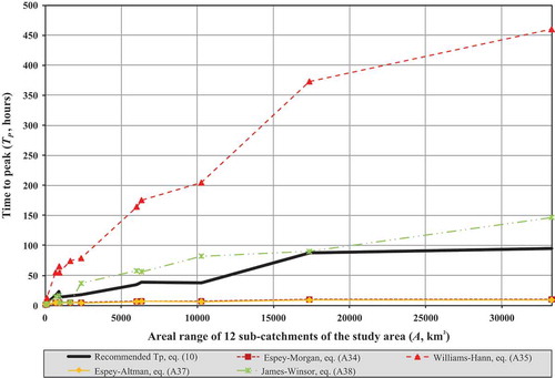
Table 9 Consistency measures for the test of T_P estimation methods compared to the “recommended method” (equation (10)).

Method	Consistency measure
	Mean recommended TP (h)	Mean estimated TP (h)	Standard bias statistic (%)	Mean error (h)	Maximum error (h)	Standard error (h)
Espey-Morgan, equation (A34)	32.3	5.4	–75.7	–26.9	–84.5	9.8
Williams-Hann, equation (A35)	32.3	143.5	295.9	111.1	365.6	4.3
Espey-Altman, equation (A37)	32.3	5.2	–74.9	–27.1	–85.4	10.5
James-Winsor, equation (A38)	32.3	42.8	9.1	10.4	52.2	11.5

Taking cognisance of the proportionality ratio between the T_C and T_L, as discussed in Section 6.3.2, it is also important to take note of the relationship between T_C, T_L and T_P by revisiting equation (10). In recognition of T_L = 0.6T_C and assuming that T_C represents the critical storm duration of which the effective rainfall is constant, while the centroid is at P_D/2, then equation (10) becomes:

(13)

where T_P is time to peak (h), and T_C is time of concentration (h).

Comparing the “mean recommended T_C” (Table 7) estimates with the “mean recommended T_P” (Table 9) estimates, resulted in a proportionality factor of 0.87, which is, in essence, almost the reciprocal of the proportionality ratio in equation (13). However, such a ratio difference, especially at a medium to large catchment scale, might imply and confirm that stream responses would most likely peak before equilibrium is reached and at a lower runoff supply rate. Consequently, this close agreement (ratio difference of 0.1) with Larson’s (1965) concept of virtual equilibrium, i.e. T_VE ≈ 0.97T_P is presumably not by coincidence. Therefore, the approximation of T_C ≈ T_P at this scale could be regarded as sufficiently accurate.

However, this relationship is based on the assumption that effective rainfall remains constant, with the critical storm duration under consideration being regarded as short; this is not the case in medium to large catchments. It is also important to note that T_P is normally defined as the time interval between the start of effective rainfall and the peak discharge of a single-peaked hydrograph, but this definition is also regarded as the conceptual definition of T_C (McCuen et al. 1984, USDA SCS 1985, Linsley et al. 1988, Seybert 2006). However, single-peaked hydrographs are more likely to occur in small catchments, while Du Plessis (1984) emphasised that T_P in medium to large catchments, could rather be expressed as the duration of the total net rise (excluding the recession limbs in-between) of a multiple-peaked hydrograph, e.g. T_P = t₁+ t₂+ t₃, if three discernible peaks are evident.

7 DISCUSSION

It was quite evident from the literature review that catchment characteristics, such as climatological variables, catchment geomorphology, catchment variables and channel geomorphology, are highly variable and have a significant influence on the catchment response time. Many researchers identified the catchment area as the single most important geomorphological variable, as it demonstrates a strong correlation with many flood indices affecting the catchment response time. Apart from the catchment area, other catchment variables, such as hydraulic and main watercourse lengths, centroid distance, average catchment and main watercourse slopes, also proved to be equally important and worth considering as predictor variables to estimate T_C, T_L and/or T_P at a medium to large catchment level.

In addition to these geomorphological catchment variables, the importance and influence of climatological and catchment variables on the catchment response time were also evident. Owing to the high variability of catchment variables at a large catchment level, the use of weighted CN values as representative predictor variables to estimate time parameters as opposed to site-specific values could be considered. Simas (1996) and Simas and Hawkins (2002), proved that CN values can be successfully incorporated to estimate lag times in medium to large catchments (see Table A2). However, weighted CN values are representative of a linear catchment response and, therefore, the use of MAP values as a surrogate for these values could be considered in order to present the nonlinear catchment responses better.

The inclusion of climatological (rainfall) variables as suitable predictors of catchment response time in South Africa has, to date, been limited to the research conducted by Schmidt and Schulze (1984), which used the two-year return period 30-min rainfall intensity variable in the SCS-SA method (equation (9)). Rainfall intensity-related variables such as this might be worth considering as catchment response time predictor variables in small catchments. However, in medium to large catchments, the antecedent soil moisture status and the quantity and distribution of rainfall relative to the attenuation of the resulting flood hydrograph as it moves towards the catchment outlet are probably of more importance than the relationship between rainfall intensity and the infiltration rate of the soil. Furthermore, the design accuracy of time parameters obtained from observed hyetographs and hydrographs depends on the computational accuracy of the corresponding observed input variables. The rainfall data in South Africa are generally only widely available at more aggregated levels, such as daily, and this reflects a paucity of rainfall data at sub-daily timescales, both in the number of rainfall gauges and length of the recorded series. Under natural conditions, especially in medium to large catchments, uniform effective rainfall seldom occurs, since both spatial and temporal variations affect the resulting runoff. Apart from the paucity of rainfall data and non-uniform distribution, time parameters for an individual event cannot always be measured directly from autographic records owing to the difficulties in determining the start time, end time and temporal and spatial distribution of effective rainfall. Problems are further compounded by poorly synchronized rainfall and runoff recorders which contribute to inaccurate time parameter estimates.

Apart from the afore-mentioned variables, the use of multiple definitions to define time parameters is regarded as also having a large influence on the inconsistency between different methods. The definitions of T_C introduced highlighted that T_C is a hydraulic time parameter, and not a true hydrograph time parameter. Hydrological literature, unfortunately, often fails to make this distinction. Time intervals from various points during a storm extracted from a hyetograph to various points on the resultant hydrograph are often misinterpreted as T_C. Therefore, these points derived from hyetographs and hydrographs should be designated as T_L or T_P. Some T_L estimates are interpreted as the time interval between the centroid of a hyetograph and hydrograph, while in other definitions the time starts at the centroid of effective rainfall, and not the total rainfall. It can also be argued that the accuracy of T_L estimation is, in general, so poor that differences in T_L starting and ending points are insignificant. The use of these multiple time parameter definitions, along with the fact that no “standard” method could be used to estimate time parameters from observed hyetographs and hydrographs, emphasises why the proportionality ratio of T_L to T_C could typically vary between 0.5 and 1 for the same catchment.

The comparison of the consistency of time parameter estimation methods in medium to large catchment areas in the C5 secondary drainage region in South Africa highlighted that, irrespective of whether an empirical time parameter estimation method (e.g. T_C, T_L or T_P) is relatively unbiased with insignificant variations compared to the recommended methods used in South Africa, the latter recommended methods would most likely also show significant variation from the observed catchment response times characterizing South African catchments. These significant variations could be ascribed to the fact that these methods have been developed and calibrated for values of the input variables (e.g. storage coefficients, channel slope, main watercourse length and/or centroid distances) that differ significantly from the pilot study area and with the values summarized in Table 4. Consequently, the use of these empirical methods must be limited to their original developmental regions, especially if no local correction factors are used, otherwise these estimates could be subjected to considerable errors. In such a case, the presence of potential observation, spatial and temporal errors/variations in geomorphological and meteorological data cannot be ignored.

However, in South Africa at this stage and catchment level, practitioners have no choice but to apply these empirical methods outside their bounds, since apart from the HRU (equation (7)) and Schmidt-Schulze (equation (9)) T_L estimation methods, none of the other methods have been verified using local hyetograph-hydrograph data. Unfortunately, not only the empirical time parameter estimation methods are used outside their bounds, but practitioners frequently also apply some of the deterministic flood estimation methods, e.g. the Rational method, beyond their intended field of application. Consequently, such practice might contribute to even larger errors in peak discharge estimation.

The inclusion or exclusion of predictor variables to establish calibrated time parameters representative of the physiographical catchment-indices influencing the temporal runoff distribution in a catchment should always be based on stepwise multiple regression analyses using the maximization of total variation and testing of statistical significance. In doing so, the temporal runoff distribution would not be condensed as a linear catchment response. Apart from the maximization of total variation and testing of statistical significance, is it also of paramount importance to take cognisance of which time parameters are actually required to improve estimates in medium to large catchments in South Africa. In design flood estimation, T_C is primarily used to estimate the critical storm duration of a specific design rainfall event used as input to deterministic methods; T_L is used in the SCS method, but the T_C could be used instead. Furthermore, calibrated T_L values are also used to re-scale the SUH method.

The estimation of either T_C or T_L from observed hyetograph-hydrograph data at a large catchment scale normally requires a convolution process based on the temporal relationship between averaged compound hyetographs (due to numerous rainfall stations) and hydrographs. Conceptually, such a procedure would assume that the volume of direct runoff is equal to the volume of effective rainfall, and that all rainfall prior to the start of direct runoff is initial abstraction, after which the loss rate is assumed to be constant. However, this simplification might ignore the “memory effect” of previous rainfall events. These compounded hyetographs also require that the degree of synchronization between point rainfall datasets be established first, after which, the conversion to averaged compound rainfall hyetographs could take place. These inherent procedural shortcomings, along with the difficulty in estimating catchment rainfall for large catchments due to the lack of continuously recorded rainfall data, as well as the problems encountered with the estimation of hyetographs and/or hydrographs centroid values at this catchment scale, emphasise that an alternative approach should be developed.

The approximation of T_C ≈ T_P could be used as basis for such an alternative approach, while the use thereof could be justified by acknowledging that, by definition, the volume of effective rainfall is equal to the volume of direct runoff/stormflow. Therefore, when separating a hydrograph into direct runoff and baseflow, the separation point could be regarded as the start of direct runoff which coincides with the onset of effective rainfall. In using such approach, the required extensive convolution process is eliminated, since T_P is directly obtained from observed streamflow data. However, it is envisaged that T_P derived from a miscellany of flood events would vary over a wide range. Consequently, factors such as antecedent moisture conditions and non-uniformities in the temporal and spatial distribution of storm rainfall have to be accounted for when flood events are extracted from the observed streamflow datasets. Upper limit T_P values and associated maximum runoff volumes would most probably be observed when the entire catchment receives rainfall for the critical storm duration. Lower limit T_P values would most likely be observed when effective rainfall of low average intensity does not cover the entire catchment, especially when a storm is centred near the outlet of a catchment.

8 CONCLUSIONS

The use of different conceptual definitions in the literature to define the interrelationship between two time variables to estimate time parameters, not only creates confusion, but also results in significantly different estimates in most cases. Evidence of such conceptual/computational misinterpretations also highlights the uncertainty involved in the process of time parameter estimation.

The parameter T_C is the most frequently used and required time parameter in flood hydrology practice, followed by T_L. In acknowledging this, as well as the basic assumptions of the approximations T_L = 0.6T_C and T_C ≈ T_P, along with the similarity between the definitions of T_P and the conceptual T_C, it is evident that the latter two time parameters should be further investigated to develop an alternative approach to estimate representative catchment response times using the most appropriate and best performing time variables and catchment storage effects.

Given the sensitivity of design peak discharges to estimated time parameter values, the use of inappropriate time variables resulting in over- or underestimated time parameters in South African flood hydrology practice highlights that considerable effort is required to ensure that time parameter estimations are representative and consistently estimated. Such over- or underestimations in the catchment response time must also be clearly understood in the context of the actual travel time associated with the size of a particular catchment, as the impact of a 10% difference in estimates might be critical in a small catchment, while being less significant in a larger catchment. However, in general terms, such under- or overestimations of the peak discharge may result in the over- or under-design of hydraulic structures, with associated socio-economic implications, which might render some projects as infeasible.

Funding

Support for this research by the National Research Foundation (NRF), University of KwaZulu-Natal (UKZN) and Central University of Technology, Free State (CUT FS) is gratefully acknowledged.

Acknowledgements

We wish to thank the anonymous reviewers for their constructive review comments, which have helped to significantly improve the paper.

APPENDIX

Table A1 Summary of T_C estimation methods used internationally.

Approach (Flow regime)	Method	Mathematical relationship	Comments
Hydraulic (Sheet overland flow)	Kinematic wave method (Morgali and Linsley 1965)	TC5 = (A1)	• This method is based on a combination of Manning’s equation and a kinematic wave approximation
		where: TC5 = time of concentration (min), i = critical rainfall intensity of duration TC (mm h^-1), LO = length of overland flow path (m), n = Manning’s roughness parameter for sheet flow (between 0.01 and 0.8), and SO = average overland slope (m m^-1).	• Assumes that the hydraulic radius of the flow path is equal to the product of travel time and rainfall intensity
			• The iterative use of this method is limited to paved areas
Hydraulic (Sheet overland flow)	NRCS kinematic wave method (Welle and Woodward 1986)	TC6 = (A2)	• This method was originally developed to avoid the iterative use of the original Kinematic wave method (equation (A1))
		where: TC6 = time of concentration (min), LO = length of overland flow path (m), n = Manning’s roughness parameter for sheet flow, P2 = 2-year return period 24-h design rainfall depth (mm), and SO = average overland slope (m m^-1).	• It is based on a power–law relationship between design rainfall intensity and duration
Empirical/Semi-analytical(Sheet overland flow)	Miller’s method (Miller 1951, ADNRW 2007)	TC7 = (A3)	• This method is based on a nomograph for shallow sheet overland flow as published by the Institution of Engineers, Australia (IEA 1977)
		where: TC7 = time of concentration (min), LO = length of overland flow path (m), n = Manning’s roughness parameter for overland flow, and SO = average overland slope (m m^-1).
Empirical/Semi-analytical (Mixed sheet/concentrated overland flow)	Federal Aviation Agency (FAA) method (FAA 1970, McCuen et al. 1984)	TC8 = (A4)	• Commonly used in urban overland flow estimations, since the Rational method’s runoff coefficient (C) is included
		where: TC8 = time of concentration (min), LO = length of overland flow path (m), C = Rational method runoff coefficient, and SO = average overland slope (m m^-1).
Empirical/Semi-analytical (Concentrated overland/ channel flow)	Eagleson’s method (Eagleson 1962, McCuen et al. 1984)	TC9 = (A5)	• This method provides an estimation of TL, i.e. the time between the centroid of effective rainfall and the peak flow rate of a direct runoff hydrograph
		where: TC9 = time of concentration (min), LO,CH = length of flow path, either overland or channel flow (m), n = Manning’s roughness parameter, R = hydraulic radius which equals the flow depth (m), and SO,CH = average overland or channel slope (m m^-1).	• A conversion factor of 1.67 was introduced to estimate TC in catchment areas smaller than ±20 km^2
			• The variables that were used during the development and calibration were based on the characteristics of a sewer system
Empirical/Semi-analytical(Concentrated overland/ channel flow)	Espey-Winslow method (Espey and Winslow 1968)	TC10 = (A6)	• According to Schulz and Lopez (1974, cited by Fang et al. 2005), this method was developed by Espey and Winslow (1968) for 17 catchments in Houston, USA
		where: TC10 = time of concentration (min), ip = imperviousness factor (%), LO,CH = length of flow path, either overland or channel flow (m), ϕ = conveyance factor, and SO,CH = average overland or channel slope (m m^-1).	• The catchment areas varied between 2.6 and 90.7 km^2 while 35% of the catchments were predominantly rural
			• Imperviousness (ip) and conveyance (ϕ) factors were introduced
			• The imperviousness factor (ip) represents overland flow retardance, while the conveyance factor (ϕ) measures subjectively the hydraulic efficiency of a watercourse/channel, taking both the condition of channel vegetation and degree of channel improvement into consideration
			• Typical ϕ values vary between 0.8 (concrete lined channels) to 1.3 (natural channels) (Heggen 2003)
Empirical/Semi-analytical (Concentrated overland/ channel flow)	Kadoya-Fukushima method (Kadoya and Fukushima 1979, Su 1995)	TC11 = (A7)	• This method is based on the kinematic wave theory and geomorphological characteristics of the slope-channel network in catchment areas between 0.5 and 143 km^2
		where TC11 = time of concentration (h), A = catchment area (km^2), CT = catchment storage coefficient (typically between 190 and 290), and iE = effective rainfall intensity (mm h^-1).	• It is physically-based with the catchment area and effective rainfall intensity incorporated to estimate TC
Empirical (Channel flow)	Bransby-Williams method(Williams 1922, Li and Chibber 2008)	TC12 = (A8)	• The use of this method is limited to rural catchment areas less than ±130 km^2 (Fang et al. 2005, Li and Chibber 2008)
		where: TC12 = time of concentration (h), A = catchment area (km^2), LCH = length of main watercourse/channel (km), and SCH = average main watercourse slope (m m^-1).	• The Australian Department of Natural Resources and Water (ADNRW 2007) highlighted that the initial overland flow travel time is already incorporated; therefore an overland flow or standard inlet time should not be added
Empirical (Channel flow)	Kirpich method (Kirpich 1940)	TC13 = (A9)	• Kirpich (1940) calibrated two empirical equations to estimate TC in small, agricultural catchments in Pennsylvania and Tennessee, USA
		where: TC13 = time of concentration (h), LCH = length of longest watercourse (km), and SCH = average main watercourse slope (m m^-1).	• The catchment areas ranged from 0.4 to 45.3 ha, with average catchment slopes between 3% and 10%
			• The estimated TC values should be multiplied by 0.4 (overland flow) and 0.2 (channel flow) respectively where the flow paths in a catchment are lined with concrete/asphalt
			• Although this method is proposed to estimate TC in main watercourses as channel flow, McCuen et al. (1984) highlighted that the coefficients used probably reflect significant portions of overland flow travel time, especially if the relatively small catchment areas used during the calibration are taken into consideration
			• The empirically-based coefficients represent regional effects, therefore the use thereof outside the calibration catchments must be limited
			• McCuen et al. (1984) also showed that this method had a tendency to underestimate TC values in 75% of the urbanized catchment areas smaller than 8 km^2, while in 25% of the catchments (8 km^2 < A ≤ 16) with substantial channel flow, it had the smallest bias
			• Pilgrim and Cordery (1993) also confirmed that the latter was also evident from studies conducted in Australia
Empirical (Channel flow)	Johnstone-Cross method (Johnstone and Cross 1949, Fang et al.  2008)	TC14 = (A10)	• This method was developed to estimate TC in the Scioto and Sandusky River catchments (Ohio Basin)
		where: TC14 = time of concentration (h), LCH = length of longest watercourse (km), and SCH = average main watercourse slope (m m^-1).	• The catchment areas ranged from 65 to 4206 km^2
			• It is primarily a function of the main watercourse length and average main watercourse slope
Empirical/Semi-analytical (Channel flow)	McCuen-Wong method (McCuen et al. 1984)	TC15 = (A11a)	• Two empirical equations were developed to estimate TC in 48 urban catchment areas less than 16 km^2
		TC15 = (A11b)	• Stepwise multiple regression analyses were used to select the predictor variables
		where: TC15 = time of concentration (h), i2 = 2-year critical rainfall intensity of duration TC (mm h^-1), LCH = length of longest watercourse (km), ϕ = conveyance factor, and SCH = average main watercourse slope (m m^-1).	• There was not a substantial difference in the goodness-of-fit (GOF) statistics of these equations
			• Equation (A11a) is preferred to estimate TC, except when the hydraulic characteristics of a main watercourse/channel differ substantially from reach to reach
			• In such cases, the conveyance factor (ϕ) should be estimated and used as input to equation (A11b)
Empirical/Semi-analytical (Channel flow)	Papadakis-Kazan method (Papadakis and Kazan 1987, USDA NRCS 2010)	TC16 = (A12)	• Data from 84 rural catchment areas smaller than ±12.4 km^2, as well as experimental data from the United States Army Corps of Engineers (USACE), Colorado State University and the University of Illinois, USA were analysed
		where: TC16 = time of concentration (h), i = critical rainfall intensity of duration TC (mm h^-1), LCH = length of longest watercourse (km), n = Manning’s roughness parameter, and SCH = average main watercourse slope (m m^-1).	• Stepwise multiple regression analyses were used to select the predictor variables from a total of 375 data points to estimate TC
Empirical (Channel flow)	Sheridan’s method (Sheridan 1994, USDA NRCS 2010)	TC17 = (A13)	• Sheridan (1994) performed a study on nine catchment areas of between 2.6 and 334.4 km^2 in Georgia and Florida, USA
		where: TC17 = time of concentration (h), and LCH = length of longest watercourse (km).	• Multiple regression analyses were performed using geomorphological catchment parameters to estimate TC
			• The main watercourse/channel length proved to be the overwhelming characteristic that correlated with TC
			• On average, the coefficient of determination (r^2) equalled 0.96
Empirical (Channel flow)	Thomas-Monde method (Thomas et al. 2000)	TC18 = (A14)	• Thomas et al. (2000) estimated average TC values for 78 rural and urban catchment areas of 4 to 1280 km^2 in three distinctive climatic regions (Appalachian Plateau, Coastal Plain and Piedmont) of Maryland, USA
		where: TC18 = time of concentration (h), AP = 1 if the catchment is in the Appalachian Plateau, otherwise 0, CP = 1 if the catchment is in the Coastal Plain, otherwise 0, FR = forest areas (%), ip = imperviousness factor (%), LCH = length of longest watercourse (km), SCH = average main watercourse slope (m km^-1), and WB = waterbodies (lakes and ponds) (%).	• It was developed by using stepwise multiple regression analyses, i.e. transforming TC and the catchment characteristics (area, main watercourse length and average slope, %-distribution of land use and vegetation, water bodies and impervious areas) to logarithms and fitting a linear regression model to the transformed data
			• This method was compared with the catchment lag times observed by the USGS and estimated with the SCS and Kirpich methods. It overestimated the USGS values by 5%, while the two other methods were consistently lower
Empirical (Channel flow)	Colorado-Sabol method (Sabol 2008)	Rocky Mountain/Great Plains/Colorado Plateau: TC19 = (A15a)	• Sabol (2008) proposed three different empirical TC methods to be used in drainage regions with distinctive geomorphological and land-use characteristics in the State of Colorado, USA
		Rural: TC19 = (A15b)	• Stepwise multiple regression analyses were used to select the predictor variables based on the catchment geomorphology and developmental variables
		Urban: TC19 = (A15c)	• Thereafter, the catchments were grouped as: (i) Rocky Mountains, Great Plains and Colorado Plateau, (ii) rural, and (iii) urban
		where: TC = time of concentration (h), A = catchment area (km^2), ip = imperviousness factor (%), LC = centroid distance (km), LCH = length of longest watercourse (km), and SCH = average main watercourse slope (m m^-1).

Table A2 Summary of T_L estimation methods used internationally.

Approach	Method	Mathematical relationship	Comments
Empirical/Semi-analytical	Snyder’s method (Snyder 1938)	(A16)	• Snyder (1938, cited by Viessman et al. 1989; Pilgrim and Cordery 1993, McCuen 2005) developed a SUH method derived from the relationships between standard unit hydrographs and geomorphological catchment descriptors
		where: TL4 = lag time (h), CT2 = catchment storage coefficient (typically between 1.35 and 1.65), LC = centroid distance (km), and LH = hydraulic length (km).	• The catchment areas evaluated varied between 25  and 25 000 km^2 and are located in the Appalachian Highlands, USA
			• The catchment storage coefficients (CT) were established regionally and include the effects of slope and storage
			• TL is defined as the time between the centroid of effective rainfall and the time of peak discharge
Empirical	Taylor-Schwarz method (Taylor and Schwarz 1952)	(A17) where: TL5 = lag time (h), LC = centroid distance (km), LH = hydraulic length of catchment (km), and S = average catchment slope (%).	• Taylor and Schwarz (1952, cited by Chow 1964) proved that the catchment storage coefficient (CT) as used in Snyder’s method (1938) is primarily influenced by the average catchment slope • Subsequently, a revised version of Snyder’s method was proposed
			• A total of 20 catchments in the North and Middle Atlantic States, USA were evaluated• According to Linsley et al. (1988), the United States Army Corps of Engineers (USACE) developed a general expression for TL in 1958 based on the Snyder (1938) and Taylor-Schwarz (1952) methods• In this method, the average catchment slope (S, %) was replaced with the average main watercourse slope (SCH, m m^-1)• Typical CT values proposed were: 0.24 (valleys; 0–10% slopes), 0.50 (foothills; 10–30% slopes) and 0.83 (mountains; >30% slopes)
Empirical/Semi-analytical	USACE method (Linsley et al. 1988)	TL6 = (A18) where: TL6 = lag time (h), CT3 = catchment storage coefficient, LC = centroid distance (km), LH = hydraulic length of catchment (km), and SCH = average main watercourse slope (m m^-1).
Empirical	Hickok-Keppel method (Hickok et al. 1959)	TL7 = (A19)	• Rainfall and runoff records for 14 catchment areas of between 27 and 1952 ha in Arizona, New Mexico and Colorado, USA were analysed
		where: TL7 = lag time (h), D = drainage density of entire catchment (km^-1), LCSA = centroid distance of source area (km), SSA = average slope of source area (%), and WSA = average width of source area (km).	• It was established that the runoff represented by unit hydrographs is related to the spatial distribution of effective rainfall and subsequently controlled the runoff source area by using possible sub-divided catchments
			• It was also found that the slope of the runoff source areas could be useful in TL estimations, while a runoff source area was defined as that portion of the catchment with the highest average catchment slope
			• The TL estimates are significant in relating the influences of catchment variables to the hydrograph shape, with the average catchment slope more correlated than the average main watercourse slope
			• The drainage density parameter reflects the proportion of channel versus overland flow and provided thus a measure of the hydraulic efficiency of a catchment
Empirical	Kennedy-Watt method (Kennedy and Watt 1967, Heggen 2003)	TL8 = (A20)	• This method takes into consideration the distribution and extent of waterbodies (lakes, marshes and ponds) in a catchment • Multiple regression analyses were used to establish the predictor variables from the catchment geomorphology and distribution of waterbodies in the upper two-thirds of the catchments
		where: TL8 = lag time (h), A = catchment area (km^2), AW = area of waterbodies in the upper two-thirds of the catchment (km^2), LH = hydraulic length of catchment (km), and SCH = average main watercourse slope (m m^-1).
Empirical/Semi-analytical	Bell-Kar method (Bell and Kar 1969)	TL9 = (A21)	• TL is primarily dependent on the geomorphological catchment characteristics
		where: TL9 = lag time (h), CT4 = catchment storage coefficient (typically between 1 and 3.4 × 10^-4), LH = hydraulic length of catchment (km), and SCH = average main watercourse slope (m m^-1).	• Critical TL values, which are arguably suitable representatives of the critical storm duration of design rainfall were used
			• This method is a modified version of the Kirpich method
Empirical/Semi-analytical	Askew’s method (Askew 1970)	TL10 = (A22)	• The variable temporal rainfall distributions had a little effect on TL, while TL can only be correlated with the weighted mean runoff rate in a catchment
		where: TL10 = lag time (h), A = catchment area (km^2), and QWM = weighted mean runoff rate (m^3 s^-1).	• The weighted mean runoff rate was defined as the mean ratio of the total runoff rate divided by the time of occurrence of direct runoff, weighted in proportion to the direct runoff discharge rate
			• A constant exponent was used as a fixed regression coefficient to develop a means of predicting the constant term in this method, which reflects a measure of a linear model’s estimation of TL
			• A high degree of association existed between the regression constant and the catchment area
Empirical	Putnam’s method (Putnam 1972)	TL11 = (A23)	• According to Haan et al. (1994), this method was developed by Putnam (1972) for 34 catchments in North Carolina, USA
		where: TL11 = lag time (h), ip = imperviousness factor (fraction), LCH = main watercourse length (km), and SCH = average main watercourse slope (m m^-1).	• Multiple regression analyses were used to establish the predictor variables from the catchment geomorphology and degree of urbanization
			• TL is defined as the time from the centroid of effective rainfall to the centroid of direct runoff
Empirical/Semi-analytical	Rao-Delleur method (Rao and Delleur 1974, Heggen 2003, Fang et al. 2005, ADNRW 2007)	TL12 = (A24a)	• It was established that average TL values (based on the time lapse between the centroid’s of effective rainfall and direct runoff) could not be used alone for runoff estimation, since it’s depending on various geomorphological and meteorological characteristics
		TL12 = (A24b)	• Three equations based on stepwise multiple regression analyses were developed with the predictor variables only related to catchment geomorphology and developmental variables.
		TL12 = (A24c)	• It was establish that equation (A24c), which included only the catchment area and imperviousness factor (ip), is as effective as equations (A24a and A24b), which include both the main watercourse length and average catchment slope
		TL12 = (A24d)	• An additional equation (A24d) was developed to take meteorological parameters (effective rainfall and duration) also into consideration
		where: TL12 = lag time (h), A = catchment area (km^2), DPE = duration of effective rainfall (h), ip = imperviousness factor (fraction), LCH = main watercourse length (km), PE = effective rainfall (mm), and SCH = average main watercourse slope (m m^-1).	• TL is not only a unique catchment characteristic, but varies from storm to storm
Empirical	NERC method (NERC 1975)	(A25)	• The United Kingdom Flood Studies Report (UK FSR) (NERC 1975) proposed the use of this method to estimate TL in ungauged UK catchments
		where: TL13 = lag time (h), LCH = main watercourse length (km), and SCH = average main watercourse slope (m km^-1).	• TL is primarily dependent on the geomorphological catchment characteristics, e.g. main watercourse length and average slope
Empirical/Semi-analytical	CUHP method Urban Drainage and Flood Control District (UDFCD 1984, cited by Heggen 2003)	TL14 = (A26)	• This method (Colorado Urban Hydrograph Procedure) is a modified version of Snyder’s method as used in urban catchment areas between 40 and 80 ha in the State of Colorado, USA
		where: TL14 = lag time (h), CT = aip^2+bip+c, imperviousness storage coefficients, ip = imperviousness factor (%), LC = centroid distance (km), LH = hydraulic length of catchment (km), and SCH = average main watercourse slope (m m^-1).	• This method was also commonly used to derive unit hydrographs for both urban and rural catchment areas ranging from 0.36  to 13 km^2 • In catchment areas larger than 13 km^2, it is recommended that the catchment be subdivided into sub-catchments of 13 km^2 or less
Empirical	Mimikou’s method (Mimikou 1984)	TL15 = (A27)	• This method was developed for catchment areas of between 202 and 5005 km^2 in the western and north western regions of Greece
		where: TL15 = lag time (h), and A = catchment area (km^2).	• TL and unit hydrograph peaks (QP) were estimated at the catchment outlets from unit hydrographs produced by 10 mm effective rainfall and 6-h storm durations
			• Storm durations of 6 h were used in all the catchments in order to avoid the effect of variable storm durations on the variation of TL and QP values from catchment to catchment. In other words, complex areal storms of various durations were delineated in 6-h intervals according to the well known multi-period technique described in the literature (Linsley et al. 1988)
			• It was established that TL and QP associated with specific storm durations, are increasing power functions of the catchment size
			• Mimikou (1984) also emphasised that the developed regional TL relationship is only applicable to the study area
Empirical	Watt-Chow method (Watt and Chow 1985)	TL16 = (A28)	• This method is based on geomorphological data from 44 catchment areas between 0.01 and 5840 km^2 across the USA and Canada
		where: TL16 = lag time (h), LCH = main watercourse length (km), and SCH = average main watercourse slope (m m^-1).	• The main watercourse slopes ranged between 0.00121 and 0.0978 m m^-1
Empirical	Haktanir-Sezen method (Haktanir and Sezen 1990, cited by Fang et al. 2005)	TL17 = (A29)	• SUHs based on two-parameter Gamma and three-parameter Beta distributions for 10 catchments in Anatolia were developed • Regression analyses were used to establish the relationships between TL and the main watercourse length
		where:
		TL17 = lag time (h), and
		LCH = main watercourse length (km).
Analytical	Loukas-Quick method (Loukas and Quick 1996)	TL18 = (A30) where: TL18 = lag time (h), B = catchment shape factor as a ƒ(k, LCH and regressed catchment parameters), iE = effective rainfall intensity (mm h^-1), KAvg = average saturated hydraulic conductivity of soil (mm h^-1), k = main watercourse shape factor, as a ƒ(channel side slopes and bed width), and SCH = average main watercourse slope (m m^-1).	• This method estimates TL in forested mountainous catchments where most of the flow is generated through subsurface pathways
			• The data acquired from field experiments were combined with the kinematic wave equation to describe the flow generation from steep, forested hillslopes
			• The hillslope runoff was used as input to the main watercourses, where the runoff movement in the channels was described by roughness parameters and slopes that vary from point to point along the main watercourse
			• The resulting equations were integrated to obtain this method, which relates the geomorphological characteristics, effective rainfall intensity and average saturated hydraulic conductivity of a catchment to its response time through an analytical mathematical procedure
			• This method provides reliable TL estimates, however, compared to existing empirical methods (Snyder 1938, NERC 1975, Watt-Chow 1985), it underestimated TL significantly in catchment areas ranging from 3 to 9.5 km^2 in Coastal British Columbia, Canada
Empirical	McEnroe-Zhao method (McEnroe and Zhao 2001)	TL19 = (A31a) TL19 = (A31b) where: TL19 = lag time (h), ip = imperviousness factor (fraction), LCH = main watercourse length (km), RD = road density (km^-1), and SCH = average main watercourse slope (m m^-1).	• TL was estimated utilizing geomorphological catchment characteristics
			• Individual and average TL values were estimated in gauged catchments from 85 observed rainfall and runoff events at 14 different sites in Johnson County, Kansas, USA
			• Two regression equations were developed through multiple regression analyses to estimate TL in urban and developing catchments
			• The catchment and channel geomorphology were obtained from DEMs and manipulated in an ArcGIS^TM environment
			• It was established that urbanization has a major impact on TL; in fully developed catchments, TL can be as much as 50% less than in a natural catchment
			• In small urban catchments with curb-and-gutter streets and storm sewers, the TL values can even be shorter
Empirical/Semi-analytical	Simas-Hawkins method (Simas 1996, Simas and Hawkins (2002))	TL20 = (A32) where: TL20 = lag time (h), A = catchment area (km^2), CN = runoff curve number, LH = hydraulic length of catchment (km), and S = average catchment slope (m m^-1).	• TL is defined as the time difference between the centroid of effective rainfall and direct runoff and was estimated from over 50 000 rainfall–runoff events in 168 catchment areas of between 0.1 and 1412.4 ha in the USA
			• The catchments were grouped into different geographical, catchment management practice, land- use and hydrological behaviour regions to explain the variation of TL between catchments
			• Multiple regression analyses were conducted to establish the most representative TL relationship
Empirical	Folmar-Miller method (Folmar and Miller 2008)	TL21 = (A33) where: TL21 = lag time (h), and LH = hydraulic length of catchment (km).	• Multiple regression analyses were performed on TL values obtained from 10 000 direct runoff events in 52 gauged catchment areas of between 1 and 4991 ha in eight different states throughout the USA
			• It was established that TL correlates strongly (r^2 = 0.89; N = 52) with the catchment hydraulic length (LH) and therefore only this parameter was used to develop this method
			• The inclusion of any other geomorphological catchment characteristics in the method did not improve its ability to predict TL
			• This method, as well as the NRCS methods, were used to estimate TL in all the catchments, after which the results were compared with the TL values obtained from observed hyetographs and hydrographs
			• Overall, this method and the NRCS methods underestimated the TL values by 65% and 62%, respectively

Table A3 Summary of T_P estimation methods used internationally.

Approach	Method	Mathematical relationship	Comments
Empirical	Espey-Morgan method (Espey et al. 1966, cited by Fang et al. 2005)	TP2 = (A34)	• Multiple regression analyses were used to establish TP for 11 rural and 24 urban catchments in Texas, New Mexico and Oklahoma, USA
		where: TP2 = time to peak (h), LCH = main watercourse length (km), and SCH = average main watercourse slope (m m^-1).	• This method is only applicable to the large, rural catchments used during this study
Empirical	Williams-Hann method (Williams and Hann 1973, cited by Viessman et al. 1989)	TP3 = (A35)	• This method is incorporated in the problem-oriented computer language for hydrological modelling (HYMO) to simulate surface runoff from catchments
		where: TP3 = time to peak (h), A = catchment area (km^2), LH = hydraulic length of catchment (km), SCH = average main watercourse slope (m m^-1), and W = width of catchment (km).	• Regional regression analyses were used to establish TP for 34 catchment areas between 1.3 and 65 km^2 in Texas, Oklahoma, Arkansas, Louisiana, Mississippi and Tennessee, USA
Empirical/Semi-analytical	NERC method (NERC 1975)	TP4 = (A36)	• TP was related to the climate, catchment and channel geomorphology and developmental variables by using stepwise multiple regression analyses
		where: TP4 = time to peak (h), Ci = climatic index of the flood runoff potential, ip = imperviousness factor (%), LCH = main watercourse length (km), and SCH = average main watercourse slope (m km^-1).	• The average main watercourse slope and degree of imperviousness were identified as the most important variables explaining the variance of TP
			• The main watercourse length was surprisingly less critical than the degree of imperviousness due to the significant inverse correlation of main watercourse length with average slope
			• The degree of imperviousness had a direct influence on the efficiency of drainage networks, flow velocities and the proportion of total runoff due to surface runoff
Empirical/Semi-analytical	Espey-Altman method (Espey and Altman 1978)	TP5 = (A37)	• A set of regional regression equations to represent 10-min SUHs from a series of effective rainfall events were developed
		where: TP5 = time to peak (h), ip = imperviousness factor (%), LH = hydraulic length of catchment (km), ϕ = conveyance factor, and SCH = average main watercourse slope (m m^-1).	• Forty-one catchment areas of between 4 and 3885 ha were analysed
			• This method is based on the concept of Snyder’s UHs (1938)
Empirical	James-Winsor method (James et al. 1987, cited by Fang et al. 2005)	Mild slope (<5%): TP6 = (A38a) Medium slope (5–10%): TP6 = (A38b)	• 283 rainfall events were analysed in catchment areas of between 0.7 and 62 km^2 in 13 states in the USA • The climate and geomorphology in these catchments were highly variable • Only 48 catchments (31 calibration catchments and 17 verification catchments) were used in the multiple regression analyses to relate the physical catchment characteristics to TP • Three empirical equations were developed for three distinctive slope classes: mild, medium and steep
		Steep slope (>10%): TP6 = (A38c)
		where: ip = imperviousness factor (%), LH = hydraulic length of catchment (km), ϕ = conveyance factor, and SCH = average main watercourse slope (m m^-1).
Empirical	Jena-Tiwari method (Jena and Tiwari 2006)	1-hour SUH: TP7 = (A39a)	• 1-h and 2-h SUHs were developed for two catchments (158 and 69 km^2) in India based on SUH parameters such as TP, QP and TB, which are all related to the catchment and channel geomorphology
		2-hour SUH: TP7 = (A39b)	• A correlation matrix between the SUH parameters and geomorphological parameters was generated to identify the most suitable geomorphological parameters
		where: TP7 = time to peak (h), LC = centroid distance (km), and LM = maximum catchment length parallel to the principal drainage line (km).	• The best single predictor for TP was found to be the catchment hydraulic length, followed by the main watercourse length and centroid distance
			• Regression equations were developed between the individual SUH parameters and the selected geomorphological parameters

REFERENCES

- ADNRW (Australian Department of Natural Resources and Water), 2007. Queensland urban drainage manual. 2nd ed. Brisbane: Department of Natural Resources and Water.
- Alexander, W.J.R., 2001. Flood risk reduction measures: incorporating flood hydrology for Southern Africa. Pretoria: Department of Civil and Biosystems Engineering, University of Pretoria.
- Alexander, W.J.R., 2002. The standard design flood. Journal of the South African Institution of Civil Engineering, 44 (1), 26–30.
- Askew, A.J., 1970. Derivation of formulae for a variable time lag. Journal of Hydrology, 10, 225–242.
- Bell, F.C. and Kar, S.O., 1969. Characteristic response times in design flood estimation. Journal of Hydrology, 8, 173–196. doi:10.1016/0022-1694(69)90120-6
- Bondelid, T.R., McCuen, R.H., and Jackson, T.J., 1982. Sensitivity of SCS models to curve number variation. Water Resources Bulletin, 20 (2), 337–349.
- CCP (California Culvert Practice), 1955. Culvert design. 2nd ed. Sacramento: Department of Public Works, Division of Highways.
- Chow, V.T., 1964. Runoff. In: V.T. Chow, ed. Handbook of applied hydrology. New York: McGraw-Hill, Ch. 14, 1–54.
- Chow, V.T., Maidment, D.R., and Mays, L.W., 1988. Applied hydrology. New York: McGraw-Hill.
- Clark, C.O., 1945. Storage and the unit hydrograph. Transactions, American Society of Civil Engineers, 110, 1419–1446.
- CSIR (Council for Scientific and Industrial Research), 2001. GIS data: classified raster data for national coverage based on 31 land cover types. Pretoria: National Land Cover Database, Environmentek, CSIR.
- DAWS (Department of Agriculture and Water Supply), 1986. Estimation of runoff. In: J.F. La G. Matthee, et al., eds. National soil conservation manual. Pretoria: Department of Agriculture and Water Supply, Ch. 5, 5.1–5.5.4.
- Dingman, S.L., 2002. Physical hydrology. 2nd ed. New York: Macmillan Press Limited.
- Du Plessis, D.B., 1984. Documentation of the March-May 1981 floods in the southeastern Cape. Pretoria: Department of Water Affairs and Forestry, Technical Report No. TR120.
- DWAF (Department of Water Affairs and Forestry), 1995. GIS data: drainage regions of South Africa. Pretoria: Department of Water Affairs and Forestry.
- Eagleson, P.S., 1962. Unit hydrograph characteristics for sewered areas. Journal of the Hydraulics Division, ASCE, 88 (HY2), 1–25.
- Espey, W.H. and Altman, D.G., 1978. Urban runoff control planning: nomographs for 10 minute unit hydrographs for small watersheds. Washington, DC: Environmental Protection Agency, Report No. EPA-600/9-78–035.
- Espey, W.H. and Winslow, D.E., 1968. The effects of urbanisation on unit hydrographs for small watersheds, Houston, Texas, 1964–67. Austin, TX: Tracor Incorporated, Report No. 68/975U and 1006/U.
- Espey, W.H., Morgan, C.W., and Masch, F.D., 1966. A study of some effects of urbanisation on storm runoff from a small watershed. Austin, TX: Water Development Board.
- ESRI (Environmental Systems Research Institute), 2006. ArcGIS desktop help: map projections and coordinate systems. Redlands, CA: Environmental Systems Research Institute.
- FAA (Federal Aviation Agency), 1970. Airport drainage. Washington, DC: Department of Transport Advisory Circular, A/C 150-5320-5B.
- Fang, X., et al., 2005. Estimating timing parameters of direct runoff and unit hydrographs for Texas watersheds. Beaumont: Texas Department of Transportation, Department of Civil Engineering, Lamar University, Report No. 0/4696/1.
- Fang, X., et al., 2008. Time of concentration estimated using watershed parameters by automated and manual methods. Journal of Irrigation and Drainage Engineering, 134 (2), 202–211.
- Folmar, N.D. and Miller, A.C., 2008. Development of an empirical lag time equation. Journal of Irrigation and Drainage Engineering, 134 (4), 501–506. doi:10.1061/(ASCE)0733-9437(2008)134:4(501)
- Gericke, O.J., 2010. Evaluation of the SDF method using a customised design flood estimation tool. Dissertation (MSc Eng). Stellenbosch University.
- Gericke, O.J. and Du Plessis, J.A., 2011. Evaluation of critical storm duration rainfall estimates used in flood hydrology in South Africa. Water SA, 37 (4), 453–470.
- Gericke, O.J. and Du Plessis, J.A., 2012. Evaluation of the standard design flood method in selected basins in South Africa. Journal of the South African Institution of Civil Engineering, 54 (2), 2–14.
- Gericke, O.J. and Du Plessis, J.A., 2013. Development of a customised design flood estimation tool to estimate floods in gauged and ungauged catchments. Water SA, 39 (1), 67–94.
- Haan, C.T., Barfield, B.J., and Hayes, J.C., 1994. Design hydrology and sedimentology for small catchments. San Diego: Academic Press Incorporated.
- Haktanir, T. and Sezen, N., 1990. Suitability of two-parameter gamma and three-parameter beta distributions as synthetic unit hydrographs in Anatolia. Hydrological Sciences Journal, 35 (2), 167–184. doi:10.1080/02626669009492416
- Hathaway, G.A., 1945. Design of drainage facilities. Transactions of American Society of Civil Engineers, 30, 697–730.
- Heggen, R., 2003. Time of concentration, lag time and time to peak [online]. In: B. Shrestha and R. Rajbhandari, eds. Proceedings of regional training course: application of geo-informatics for water resources management. Kathmandu, Nepal: International Centre for Integrated Mountain Development. Ch. 33.1–3.23.Available from: http://www.hkh-friend.net.np/rhdc/training/lectures/heggen/Tc_3.pdf [Accessed 30 September 2010].
- Henderson, F.M. and Wooding, R.A., 1964. Overland flow and groundwater flow from a steady rainfall of finite duration. Journal of Geophysical Research, 69 (8), 1531–1540. doi:10.1029/JZ069i008p01531
- Hickok, R.B., Keppel, R.V., and Rafferty, B.R., 1959. Hydrograph synthesis for small arid-land watersheds. Journal of Agricultural Engineering ASAE, 40 (10), 608–611.
- Hood, M.J., Clausen, J.C., and Warner, G.S., 2007. Comparison of stormwater lag times for low impact and traditional residential development. Journal of the American Water Resources Association, 43 (4), 1 036–1 046. doi:10.1111/j.1752-1688.2007.00085.x
- HRU (Hydrological Research Unit), 1972. Design flood determination in South Africa. Johannesburg: Hydrological Research Unit, University of the Witwatersrand, Report No. 1/72.
- IEA (Institution of Engineers, Australia), 1977. Australian rainfall and runoff: flood analysis and design. 2nd ed. Canberra: IEA.
- James, W.P., Winsor, P.W., and Williams, J.R., 1987. Synthetic unit hydrographs. Journal of Water Resources Planning and Management, 113 (1), 70–81.
- Jena, S.K. and Tiwari, K.N., 2006. Modeling synthetic unit hydrograph parameters with geomorphologic parameters of watersheds. Journal of Hydrology, 319, 1–14. doi:10.1016/j.jhydrol.2005.03.025
- Johnstone, D. and Cross, W.P., 1949. Elements of applied hydrology. New York: Ronald Press.
- Kadoya, M. and Fukushima, A., 1979. Concentration time of flood runoff in smaller river basins. In: H.J. Morel-Seytoux, et al., eds. Proceedings of the 3rd International Hydrology Symposium on theoretical and applied hydrology. Fort Collins: Water Resources Publication, Colorado State University, 75–88.
- Kennedy, R.J. and Watt, W.E., 1967. The relationship between lag time and the physical characteristics of drainage basins in Southern Ontario. In: Floods and their computations. Leningrad symposium 1967. Oxfordshire: International Association of Hydrological Sciences, IAHS Publ. 85. 866–874.
- Kerby, W.S., 1959. Time of concentration for overland flow. Civil Engineering, 29 (3), 174.
- Kirpich, Z.P., 1940. Time of concentration of small agricultural watersheds. Civil Engineering, 10 (6), 362.
- Larson, C.L., 1965. A two phase approach to the prediction of peak rates and frequencies of runoff for small ungauged watersheds. Stanford: Department of Civil Engineering, Stanford University, Technical Report No. 53.
- Li, M. and Chibber, P., 2008. Overland flow time of concentration on very flat terrains. Transportation Research Record: Journal of the Transportation Research Board, 2060, 133–140. doi:10.3141/2060-15
- Linsley, R.K., Kohler, M.A., and Paulhus, J.L.H., 1988. In: S.I. Metric ed. Hydrology for engineers. Singapore: McGraw-Hill.
- Loukas, A. and Quick, M.C., 1996. Physically-based estimation of lag time for forested mountainous watersheds. Hydrological Sciences Journal, 41 (1), 1–19. doi:10.1080/02626669609491475
- Lynch, S.D., 2004. Development of a raster database of annual, monthly and daily rainfall for Southern Africa. Pretoria: Water Research Commission, WRC Report No. 1156/1/04.
- McCuen, R.H., 2005. Hydrologic analysis and design. 3rd ed. New York: Prentice-Hall.
- McCuen, R.H., 2009. Uncertainty analyses of watershed time parameters. Journal of Hydrologic Engineering, 14 (5), 490–498. doi:10.1061/(ASCE)HE.1943-5584.0000011
- McCuen, R.H. and Spiess, J.M., 1995. Assessment of kinematic wave time of concentration. Journal of Hydraulic Engineering, 121 (3), 256–266.
- McCuen, R.H., Wong, S.L., and Rawls, W.J., 1984. Estimating urban time of concentration. Journal of Hydraulic Engineering, 110 (7), 887–904.
- McEnroe, B.M. and Zhao, H., 2001. Lag times of urban and developing watersheds in Johnson County, Kansas. Kansas: University of Kansas, Report No. KTRAN: KU–99–5.
- Midgeley, D.C., Pitman, W.V., and Middleton, B.J., 1994. Surface water resources of South Africa. Volume 2, Pretoria: Water Research Commission, Drainage Region C.WRC Report No. 298/2.1/94.
- Miller, W.C., 1951. Evolving a shortcut for design of storm sewers. Municipal Utilities, 89 (9), 42–54.
- Mimikou, M., 1984. Regional relationships between basin size and runoff characteristics. Hydrological Sciences Journal, 29 (1), 63–73. doi:10.1080/02626668409490922
- Mockus, V., 1957. Use of storm and watershed characteristics in synthetic hydrograph analysis and application. Washington, DC: USDA SCS.
- Morgali, J.R. and Linsley, R.K., 1965. Computer simulation of overland flow. Journal of Hydraulics Division ASCE, 91 (HY3), 81–100.
- NERC (Natural Environmental Research Council), 1975. Flood studies report. London: Natural Environment Research Council.
- Papadakis, K.N. and Kazan, M.N., 1987. Time of concentration in small rural watersheds. In: Proceedings of the ASCE engineering hydrology symposium. Williamsburg, VA: ASCE, 633–638.
- Pavlovic, S.B. and Moglen, G.E., 2008. Discretization issues in travel time calculations. Journal of Hydrologic Engineering, 13 (2), 71–79. doi:10.1061/(ASCE)1084-0699(2008)13:2(71)
- Pegram, G.G.S. and Parak, M., 2004. A review of the regional maximum flood and rational formula using geomorphological information and observed floods. Water SA, 30 (3), 377–392.
- Pilgrim, D.H. and Cordery, I., 1993. Flood runoff. In: D.R. Maidment, ed. Handbook of hydrology. New York: McGraw-Hill, Ch. 9, 1–42.
- Pullen, R.A., 1969. Synthetic Unitgraphs for South Africa. Johannesburg: Hydrological Research Unit, University of the Witwatersrand, Report No. 3/69.
- Putnam, A.L., 1972. Rainfall and runoff in urban areas: a case study of flooding in the Piedmont of North Carolina. In: Proceedings of the Urban Rainfall Management Problems Conference, 17–18 April. Lexington: University of Kentucky.
- Ramser, C.E., 1927. Runoff from small agricultural areas. Journal of Agricultural Engineering, 34 (9), 797–823.
- Rao, A.R. and Delleur, J.W., 1974. Instantaneous unit hydrographs, peak discharges and time lags in urban basins. Hydrological Sciences Bulletin, 19 (2), 185–198. doi:10.1080/02626667409493898
- Reich, B.M., 1962. Soil conservation service design hydrographs. Transactions of South African Institute of Civil Engineers, 4 (May), 1962.
- Royappen, M., et al., 2002. An analysis of catchment attributes and hydrological response characteristics in a range of small catchments. Pretoria: Water Research Commission, WRC Report No. 1193/01/02.
- Sabol, G.V., 1993. Lag relations for semi-arid regions and urban areas. In: Proceedings of the ASCE engineering hydrology symposium. San Francisco, CA: ASCE, 168–173.
- Sabol, G.V., 2008. Hydrologic basin response parameter estimation guidelines. Scottsdale, AZ: Dam Safety Report, Tierra Grande International Incorporated, State of Colorado.
- SANRAL (South African National Roads Agency Limited), 2013. Drainage manual. 6th ed. Pretoria: South African National Roads Agency Limited.
- Schmidt, E.J. and Schulze, R.E., 1984. Improved estimation of peak flow rates using modified SCS lag equations. Pietermaritzburg: Department of Agricultural Engineering, University of Natal, ACRU Report No. 17.
- Schultz, G.A., 1964. Studies in flood hydrograph synthesisation. Dissertation (MSc). University of the Witwatersrand.
- Schulz, E.F. and Lopez, O.G., 1974. Determination of urban watershed response time. Fort Collins: Colorado State University.
- Schulze, R.E., Schmidt, E.J., and Smithers, J.C., 1992. SCS-SA user manual: PC-based SCS design flood estimates for small catchments in Southern Africa. Pietermaritzburg: Department of Agricultural Engineering, University of Natal, ACRU Report No. 40.
- Seybert, T.A., 2006. Stormwater management for land development: methods and calculations for quantity control. Hoboken, NJ: John Wiley and Sons Incorporated.
- Sheridan, J.M., 1994. Hydrograph time parameters for flatland watersheds. Transactions of American Society of Agricultural Engineers, 37 (1), 103–113. doi:10.13031/2013.28059
- Simas, M.J.C., 1996. Lag time characteristics in small watersheds in the United States. Thesis (PhD). University of Arizona.
- Simas, M.J.C. and Hawkins, R.H., 2002. Lag time characteristics in small watersheds in the United States. In: Proceedings of the 2nd federal interagency hydrologic modelling conference. Las Vegas, Nevada: FIHMC, 1–7.
- Smithers, J.C. and Schulze, R.E., 2000. Long duration design rainfall estimates for South Africa. Pretoria: Water Research Commission, WRC Report No. 811/1/00.
- Snyder, F.F., 1938. Synthetic unit hydrographs. Transactions, American Geophysical Union, 19, 447.
- Su, D.H. and Fang, X., 2004. Estimating travelling time of flat terrain by two-dimensional overland flow model. In: G.H. Jirka and W.S.J. Uijttewaal, eds. Shallow flows. Rotterdam: A.A. Balkema, 629–635.
- Taylor, A.B. and Schwarz, H.E., 1952. Unit hydrograph lag and peakflow related to basin characteristics. Transactions, American Geophysical Union, 33, 235–246. doi:10.1029/TR033i002p00235
- Thomas, W.O., Monde, M.C., and Davis, S.R., 2000. Estimation of time of concentration for Maryland streams. Journal of the Transportation Research Board, 1720, 95–99.
- UDFCD (Urban Drainage and Flood Control District), 1984. Urban storm drainage criteria user’s manual. Revised ed. Denver, CO: Denver Regional Council of Governments.
- USBR (United States Bureau of Reclamation), 1973. Design of small dams. 2nd ed. Washington, DC: Water Resources Technical Publications.
- USDA NRCS (United States Department of Agriculture Natural Resources Conservation Service), 2010. Time of concentration. In: D.E. Woodward, et al., eds. National engineering handbook. Washington, DC: USDA, Ch. 15 (Section 4, Part 630), 1–18.
- USDA SCS (United States Department of Agriculture Soil Conservation Service), 1985. Hydrology. In: K.M. Kent, et al., eds. National engineering handbook. Washington, DC: USDA, Section 4.
- USGS (United States Geological Survey), 2002. SRTM topography [online]. USGS. Available from: http://dds.cr.usgs.gov/srtm/version2_1/Documentation/SRTM_Topo.pdf [Accessed 2 June 2010].
- Van der Spuy, D. and Rademeyer, P.F., 2010. Flood frequency estimation methods as applied in the Department of Water Affairs. Pretoria: Department of Water Affairs.
- Viessman, W., Lewis, G.L., and Knapp, J.W., 1989. Introduction to hydrology. 3rd ed. New York: Harper and Row Publishers Incorporated.
- Viessman, W. and Lewis, G.L., 1996. Introduction to hydrology. 4th ed. New York: Harper Collins College Publishers Incorporated.
- Watt, W.E. and Chow, K.C.A., 1985. A general expression for basin lag time. Canadian Journal of Civil Engineering, 12, 294–300.
- Welle, P.I. and Woodward, D., 1986. Engineering hydrology time of concentration. Pennsylvania: Technical Release, USDA SCS Engineering Division.
- Williams, G.B., 1922. Flood discharges and the dimensions of spillways in India. Engineering (London), 134, 321.
- Williams, J.R. and Hann, R.W.J., 1973. HYMO: problem-oriented computer language for building hydrologic models. Water Resources Research, 8 (1), 79–86.
- Wong, T.S.W. and Chen, C.N., 1997. Time of concentration formula for sheet flow of varying flow regime. Journal of Hydrologic Engineering, 2 (3), 136–139. doi:10.1061/(ASCE)1084-0699(1997)2:3(136)
- Woolhiser, D.A. and Liggett, J.A., 1967. Unsteady, one-dimensional flow over a plane-the rising hydrograph. Water Resources Research, 3 (3), 753–771. doi:10.1029/WR003i003p00753