Investigating the uncertainty and transferability of parameters in SWAT model under climate change

ABSTRACT

There is an implicit assumption in most work that the parameters calibrated based on observations remain valid for future climatic conditions. However, this might not be true due to parameter instability. This paper investigates the uncertainty and transferability of parameters in a hydrological model under climate change. Parameter transferability is investigated with three parameter sets identified for different climatic conditions, which are: wet, intermediate and dry. A parameter set based on the baseline period (1961–1990) is also investigated for comparison. For uncertainty analysis, a k-simulation set approach is proposed instead of employing the traditional optimization method which uses a single best-fit parameter set. The results show that the parameter set from the wet sub-period performs the best when transferred into wet climate condition, while the parameter set from the baseline period is the most appropriate when transferred into dry climate condition. The largest uncertainty of simulated daily high flows for 2011–2040 is from the parameter set trained in the dry sub-period, while that of simulated daily medium and low flows lies in the parameter set from the intermediate calibration sub-period. For annual changes in the future period, the uncertainty with the parameter set from the intermediate sub-period is the largest, followed by the wet sub-period and dry sub-period. Compared with high and medium flows/runoffs, the uncertainty of low flows/runoffs is much smaller for both simulated daily flows and annual runoffs. For seasonal runoffs, the largest uncertainty is from the intermediate sub-period, while the smallest is from the dry sub-period. Apart from that, the largest uncertainty can be observed for spring runoffs and the lowest one for autumn runoffs. Compared with the traditional optimization method, the k-simulation set approach shows many more advantages, particularly being able to provide uncertainty information to decision support for watershed management under climate change.

EDITOR Z.W. Kundzewicz ASSOCIATE EDITOR not assigned

KEYWORDS:

• parameter transferability
• uncertainty
• calibration
• climate change

1 Introduction

As reported by IPCC (2007), the global average surface temperature has increased by approximately 0.6°C and is projected to rise by an additional 1.1–6.4°C over the 21st century. Climate change influences precipitation, storm patterns and sea level, which makes watershed management a great challenge for decision makers.

Hydrological models forced with regional climate change scenarios downscaled from global climate models (GCMs) are widely employed to assess the impacts of climate change at the catchment scale (Bastola et al. 2011b, Tian et al. 2013). Physically-based hydrological models are more suitable for simulations of basin response to a changing climate than empirical or conceptual models which rely more heavily on parameters calibration (Ragettli and Pellicciotti 2012). However, problems with a priori estimation of model parameters make physically-based hydrological models difficult to apply, while conceptual models are often argued to be a more practical alternative (Piniewski et al. 2013). Parameters employed in hydrological models (e.g. semi-distributed models) to simulate flows of the future period are often acquired by calibration. Calibration is done with observed data in a particular period, which results in a doubt whether the parameters obtained in the calibration period can be transferred for use in the other periods or not. Particularly in a non-stationary condition, transferability of parameters becomes questionable (Vaze et al. 2010).

Compared with the works about spatial parameter transferability (Van Der Linden and Woo 2003, Gan and Burges 2006, Mittman et al. 2012), the studies about temporal parameter transferability are much fewer. Apaydin et al. (2006) recommended updating calibrated model parameters whenever marked changes occurred in the watershed. Vaze et al. (2010) investigated whether the calibrated parameter values based on historical observed data can be used to reliably predict runoff responses to changes in the future climate inputs. They concluded that when the data used for calibration was more than 20 years, the calibrated parameters could be used for climate impact studies where the future mean annual rainfall was not more than 15% drier or 20% wetter than the mean annual rainfall in the model calibration period. Bastola et al. (2011a) evaluated the transferability of hydrological model parameters for simulations under changed climatic conditions by using a simple threshold-based approach that related behavioural sets of parameters to climatic conditions. Their results suggested that the issue of time invariance in the value of parameters had a minimal effect on the simulation if the change in precipitation was less than 10% of the data used for calibration. Coron et al. (2012) investigated the actual extrapolation capacity of three hydrological models in differing climate conditions, and they found that calibration over a wetter (drier) climate than the validation climate leads to an overestimation (underestimation) of the mean simulated runoff; meantime, transfer of model parameters in time may introduce a significant level of errors in simulation.

All the works mentioned above and almost all studies about the temporal transferability of hydrological model parameters just employed the single best-fit parameter set associated with the highest individual objective function score. But single best-fit calibration contains high risks of overfitting and lack of critical uncertainty information. Among those studies about parameter transferability, much less work has been done about uncertainty analysis of parameters. Beven (2006) argued that the potential for multiple acceptable models as representations of hydrological and other environmental systems (the equifinality thesis) should be given more serious consideration than hitherto. Many works have also emphasized the importance of parameter uncertainty in hydrological modelling under both stationary and non-stationary conditions. Bastola et al. (2011b) argued that the role of uncertainty stemming from hydrological model uncertainty (parameter and structural uncertainty) in climate impact studies may be remarkably high and should be routinely considered in impact studies. Brigode et al. (2013) investigated the uncertainty of hydrological predictions due to rainfall–runoff model parameters in the context of climate change impact studies. Two sources of uncertainty were considered, which are dependence of the optimal parameter set on the climate characteristics of the calibration period and use of several posterior parameter sets over a given calibration period. They concluded that the first source was the major source of variability in streamflow projections in future climate conditions for GR4J rainfall–runoff model and TOPMO model.

Another deficiency of these studies is that most of them were done with lumped hydrological models. However, it is often assumed that spatially explicit distributed hydrological models are more suited to predict the effects of changing environmental conditions (Beven and Binley 1992). The use of semi-distributed and distributed hydrological models in climate change impact analysis is increasing all the time (Maurer et al. 2010, Piniewski et al. 2013, Xu et al. 2013). The Soil and Water Assessment Tool (SWAT) model is used in this study. It is chosen because it is a very commonly used and well-supported model (Easton et al. 2008). The SWAT model is a physically-based and semi-distributed hydrological model based on a daily or sub-daily time step (Arnold et al. 1998). This paper intends to use this model to investigate the temporal transferability of a semi-distributed hydrological model’s parameters and to quantify runoff changes caused by parameter transferability in the future. Considering the uncertainty of parameters, a new simulation set approach is proposed to analyse changes of simulated hydrological responses and uncertainties in simulated flows.

2 Study area and data

2.1 Study area

The Qu River basin is located in Zhejiang Province in eastern China, which is the sub-basin of the Qiantang River basin. The Qiantang River basin is the largest and longest River system in Zhejiang Province, which passes through the provincial capital Hangzhou, before flowing into the East China Sea through Hangzhou Bay. The Qu River basin is located in the southwest of the Qiantang River basin, and its surface area is 5690 km². The climate of the Qu River basin is dominated by humid subtropical monsoon where there are four well marked seasons, moderate temperature, plentiful rainfall and sunshine, long periods of winter and summer and short periods of spring and autumn. Its annual average total precipitation is 1500 mm and the average temperature is about 15–18°C. The monthly regimes of temperature, precipitation and streamflow from 1961 to 2006 at Quzhou station, the outlet of the Qu River basin (Fig. 1) are presented in Fig. 2.

Figure 1. Location of the outlet station, Quzhou and distributions of meteorological stations, precipitation and discharge stations.

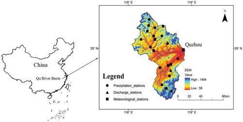
Figure 2. Monthly regimes of temperature, precipitation and streamflow at the outlet of the Qu River basin.

2.2 Data used in this study

There are 18 precipitation stations, six discharge stations and three meteorological stations in the study area (Fig. 1). Daily precipitation, maximum and minimum temperature values are used as input data for the SWAT model. Three meteorological stations are used to set up weather generator for SWAT. Other input data requirements for the SWAT model include digital elevation model, land cover, and spatial coverage of soil. A 90 m by 90 m resolution digital elevation model (DEM) is downloaded from NASA (National Aeronautics and Space Administration) Shuttle Radar Topographic Mission (http://srtm.csi.cgiar.org/). Land cover data are obtained from 1 km by 1 km Global Land Cover 2000 (http://bioval.jrc.ec.europa.euproducts/glc2000/products.php). The land cover data were reclassified into 10 types according to the land cover database requirement. The resolution of soil data is also 1 km by 1 km, which is available at the Harmonized World Soil Database (http://www.iiasa.ac.at/Research/LUC/External-World-soil-database/HTML/). As the downloaded soil database consists of soil types for the USA, the soil data are reclassified according to the China Soil Classification. Afterwards, the soil was divided into two layers as the original soil data contained just two layers.

2.3 Future climate change scenarios

Statistical downscaling and dynamic downscaling (e.g. regional climate model, RCM) are two ways to derive regional or station-scale future climate change projections. Many studies about comparative analysis of different downscaling methods have been done (Haylock et al. 2006, Schmidli et al. 2007, Gutmann et al. 2012). As regional climate models are based on physical processes, they have advantages over other statistical downscaling methods in terms of simulating extreme events (Zhang et al. 2014). Therefore, a regional climate model PRECIS (Providing Regional Climates for Impacts Studies, http://www.metoffice.gov.uk/precis/) is used to downscale meteorological data from global climate models. It was developed by the Met Office Hadley Centre, UK, and can be used to generate detailed climate change projections in any region of the world.

From 2011 to 2040, daily precipitation, maximum and minimum temperature values are simulated by the PRECIS model driven by two different GCMs (global climate model), each with one emission scenario (A1B). The scenario A1B assumes rapid economic and population growth that peaks mid-century and declines thereafter. The A1B scenario is considered realistic in China, which is located in East Asia, and it ensures the most robust pattern of climate change is captured instead of using A2 or B2 (Hori and Ueda 2006). Two representative GCMs are chosen as boundary data of the regional climate model: HadCM3 (UK Met Office Hadley Centre Coupled Model version 3) and ECHAM5 (European Centre-Hamburg model version 5). The reason why these two GCMs are chosen is that they have been proved to be capable of properly simulating the East Asian Monsoon on the basis of criteria (e.g. correlation coefficient and skill scores of precipitation) (Min et al. 2004, Kitoh and Uchiyama 2006). Xu et al. (2012) used HadCM3 and ECHAM5 to project future climate change in the Qiantang River Basin. HadCM3 combines atmosphere and ocean components and is one of the major models used in the IPCC Third and Fourth Assessment Reports. Its horizontal resolution is 3.75 degrees of longitude by 2.5 degrees of latitude (Gordon et al. 2000). ECHAM5 is the fifth-generation atmospheric general circulation model and the latest version in the series of ECHAM models. Its atmospheric resolution is 2.8 degrees of longitude by 2.8 degrees of latitude (Roeckner et al. 2003).

The spatial resolution of PRECIS outputs is 0.25 degrees latitude by 0.25 degrees longitude, and the temporal resolution is daily. Although RCMs are widely used for providing regional climate information, they still feature considerable systematic errors. Therefore, bias correction of RCM outputs is a prerequisite step of most climate change impact studies. Bias correction is a statistical approach that seeks to use information from biased model outputs (Chen et al. 2013). Many sophisticated RCM bias correction methods have been proposed and evaluated. Among them, Themeßl et al. (2011) concluded that quantile mapping (QM) outperforms all other investigated empirical statistical downscaling and error correction methods. Themeßl et al. (2012) used an upgraded QM method to correct future climate change projections from the regional climate model PRECIS. In order to provide reliable future climate change projections (2011–2040) for the Qu River basin, the outputs from PRECIS are bias-corrected via a quantile mapping (QM) method from Themeßl et al. (2012) to reduce the bias from the regional climate model.

3 Methodology

This section describes how the work is done in detail. Figure 3 presents the methodology for this study.

Figure 3. Conceptual diagram of SWAT model calibration scheme. LH-OAT: Latin-Hypercube and One-factor-At-a-Time sampling, NS: Nash-Sutcliffe efficiency.

3.1 SWAT hydrological model and sensitivity analysis

The SWAT model is used to simulate daily flows from 1961 to 2006 at Quzhou station, located at the outlet of the whole watershed (Fig. 1). The SWAT model generally divides the watershed into smaller sub-basins and requires input data such as soil and land use for each sub-basin. In the SWAT model, a Hydrologic Response Unit (HRU) is a basic computational unit assumed to be homogeneous in hydrologic response to land cover change. The Qu River basin is divided into 46 sub-basins and 262 HRUs. The Hargreaves method is used to estimate potential evapotranspiration (Hargreaves and Samani 1985). Several SWAT applications (Wang et al. 2006, Setegn et al. 2008) have shown that the Hargreaves method produces much better uncalibrated fits than the Penman-Monteith method between simulated and observed flows, at low flow especially. Sensitivity analysis is accomplished for 27 parameters that may have a potential to influence River flow with LH-OAT (Latin-Hypercube and One-factor-At-a-Time sampling) method (Van Griensven et al. 2006). All the available observed flows from 1961 to 2006 in the outlet of the watershed, Quzhou station, are used in the sensitivity analysis.

3.2 Calibration sub-periods and validation periods

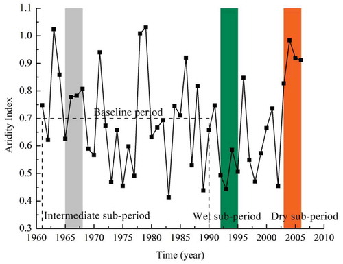
In order to evaluate the parameter transferability under changing climatic conditions, four sets of calibration data are selected representing periods where each dataset defines different climatic periods, namely wet, intermediate, dry and baseline period (Wilby 2005, Bastola et al. 2011a, Brigode et al. 2013). Any climate scenario must adopt a reference baseline from which to calculate changes in climate. According to IPCC (2007), the period from 1961 to 1990 is used as the baseline period, which is sufficiently long to cover wet, intermediate and dry periods. Some works have been done about how to characterize the climatic characteristics of each sub-period. Brigode et al. (2013) chose the aridity index defined as the ratio of mean Penman potential evapotranspiration to mean precipitation to characterize the climatic specificity of sub-periods. Bastola et al. (2011a) selected three sub-periods representing different climatic characters based upon a selected threshold for annual average rainfall. In this paper, aridity index is used to select sub-periods (Fig. 4). Because of the constraints of available measured data, it is difficult to select consecutive years whose aridity indexes lie in the range corresponding to the same climatic condition. Therefore, in this study, 4 years and 2 years are set as fixed lengths for the calibration period and the validation period, respectively. It turns out that the wet sub-period is from 1992 to 1995, the intermediate sub-period is from 1965 to 1968 and the dry sub-period is from 2003 to 2006. Quantified hydroclimatic differences between the three sub-periods and the aridity index are presented in Table 1. To analyse the dependence of model performance on the climatic characteristics of the calibration period, two validation periods under different future projections are used. The period whose aridity index is the closest to the future condition is identified as the validation period according to Brigode et al. (2013). They chose the driest sub-period as the validation period because the selected climate projection indicates that future conditions will be drier and warmer on the test basin. Via calculation, it is found that the aridity index from 2011 to 2040 under HadCM3 and ECHAM5 is 0.58 and 1.02, respectively. The reason why the difference between the aridity index values under HadCM3 and ECHAM5 is so large is that precipitation data generated by ECHAM5 are much lower than that by HadCM3. Thus the period from 1969 to 1970 is used as the validation period under HadCM3, whose average aridity is 0.58. The period from 1978 to 1979 is used as the validation period under ECHAM5, whose average aridity is 1.02.

Table 1. Aridity index and main hydrological differences between the wet, intermediate and dry sub-periods.

Sub-period	Q (m^3/s)	PET (mm)	P (mm)	Aridity index
Wet	262.07	998.06	1980.45	0.51
Intermediate	176.08	1165.35	1567.85	0.75
Dry	161.86	1208.25	1334.03	0.91

Figure 4. Calibration sub-periods. Wet sub-period (green): 1992–1995; intermediate sub-period (grey): 1965–1968; dry sub-period (orange): 2003–2006; baseline period (dashed line): 1961–1990.

3.3 Calibration and validation process

After sensitivity analysis by LH-OAT, 10 parameters are identified as sensitive ones. Among them, SOL_K and SOL_Z of the two soil layers are calibrated separately, which results in 12 parameters used in the following calibration and validation (Table 2). Realistic initial ranges for each parameter are defined based on existing work in the study area (Table 2) (Xu et al. 2013). The optimization program SUFI-2 (Sequential Uncertainty Fitting Ver.2) (Abbaspour et al. 2007) in SWAT-CUP (SWAT Calibration and Uncertainty Procedures) (Abbaspour 2007) is employed to do the calibration. Three climatically contrasted sub-periods (wet, intermediate and dry) and the baseline period are used in the calibration and one year warm-up period is considered for each simulation. This means there are four separate calibration processes, each with 12 parameters in one calibration sub-period. Latin hypercube sampling (LHS) is used to generate multidimensional parameter value combinations across a set of 1000 simulations with uniform distributions for each sub-period. After the first iteration, a new parameter range is suggested by the SUFI-2 algorithm, which then is used as input range for the next iteration. The objective function used to evaluate calibration efficiency is Nash-Sutcliffe (NS) coefficient (Nash and Sutcliffe 1970) (equation (1)). For NS, a threshold of behavioural simulation is 0.5. A value between 0.5 and 0.7 indicates a good performance, and a value greater than 0.7 indicates a very good performance. The threshold has been previously shown to be useful in other calibration works (Mishra et al. 2010, Safeeq and Fares 2012). Overestimation bias in percentage (PBIAS) (equation (2)) and mean absolute error (MAE) (equation (3)) are also calculated to evaluate calibration efficiency. The PBIAS is used to measure the average tendency of the simulated data to be larger or smaller than the observed counterparts. The optimal value of PBIAS is zero, with positive (negative) values indicating model overestimation (underestimation) bias (Zhang et al. 2011). The MAE is used to describe average model performance error and represent average difference when no set of estimates is known to be the most reliable (Willmott and Matsuura 2005).

(1)

(2)

(3)

Table 2. SWAT calibration parameters’ initial ranges and calibration ranges in the third iteration.

Parameter	Description	Unit	Initial range	Wet sub-period	Intermediate sub-period	Dry sub-period	Baseline period
SURLAG^v	Surface runoff lag time	days	[0,10]	[0,2.67]	[0,3.09]	[0,2.8]	[0,3.14]
CH_K2^v	Effective hydraulic conductivity in main channel alluvium	mm/h	[0,150]	[107.24,150.00]	[102.67,150]	[111.21,150]	[90.28,130.1]
CN2^a	Initial SCS runoff curve number for moisture condition II	——	[54,80]	[72.96,80.00]	[70.81,80]	[54.00,63.08]	[71.37,80]
ALPHA_BF^v	Baseflow alpha factor	days	[0,1]	[0.67,1]	[0.68,1]	[0.57,0.86]	[0.7,1]
CH_N2^v	Manning coefficient for channel	——	[0,0.3]	[0.22,0.30]	[0.21,0.3]	[0,0.12]	[0.22,0.3]
ESCO^v	Soil evaporation compensation factor	——	[0.01,1]	[0.34,0.78]	[0.66,1]	[0.67,1]	[0.08,0.57]
SOL_AWC()^r	Available soil water capacity	——	[0,0.92]	[0.67,0.92]	[0,0.34]	[0.16,0.25]	[0.32,0.7]
CANMX^v	Maximum canopy index	mm	[0,10]	[4.91,8.30]	[4.56,8.19]	[2.68,7.51]	[0,3.45]
SOL_K(1)^r	Saturated hydraulic conductivity of the first soil layer	mm/h	[0,100]	[45.81,68.00]	[62.50,92.65]	[64,84]	[51.93,83.98]
SOL_K(2)^r	Saturated hydraulic conductivity of the second soil layer	mm/h	[0,100]	[0,21.00]	[48.47,86.96]	[71,101]	[19.54,58.64]
SOL_Z(1)^r	Soil depth of the first soil layer	mm	[0,3000]	[0,842.66]	[0,1051.96]	[530.7,540]	[1184.56,2394.97]
SOL_Z(2)^r	Soil depth of the second soil layer	mm	[0,3000]	[653.86,2001.64]	[1853.78,2941.34]	[1000,1812.22]	[1999,3000]

^v means the existing parameter value is to be replaced by the given value; ^a means the given value is added to the exsiting parameter value; and ^r means the exsiting parameter value is multiplied by (1 + a given value).

where , , and are the measured, simulated and mean of measured values, respectively, and N is the total number of data points in the simulation.

According to the iterative calibration design, as iteration goes by, each parameter range narrows, resulting in the narrowing of distribution of simulated flows. Therefore, for uncertainty analysis, the iterations cannot be too many times. After three iterations, the numbers of behaviour simulations for the wet, intermediate and dry sub-periods and the baseline period are 981, 1000, 792 and 946, respectively, which are almost up to 80% of the overall 1000 simulations. For further uncertainty analysis, the number of behavioural simulations exceeding 80% of the total simulations is considered rational. Compared with the other three calibration periods, the behaviour simulations of the dry sub-period is slightly less, thus one more iteration in the dry sub-period is done, and the number of behaviour simulations becomes 834. The number of behavioural simulations does not change so much but the parameter range narrows a lot. This narrowing leads to lower variability within the simulation set. Therefore, a satisfying stopping rule is chosen to be three iterations. Thus the hydrological model runs three iterations in all the sub-periods. Parameter sets corresponding to behaviour simulation are used to generate simulated flows in the validation period and future flows from 2011 to 2040 under HadCM3 and ECHAM5. Such approach is called k-simulation set approach in this study.

3.4 Parameter instability and uncertainty analysis

Annual average flows and seasonal runoffs are calculated to analyse the impact of parameter instability. 95% prediction uncertainties (95PPU) of simulated flows from 2011 to 2040 are calculated for uncertainty analysis. The 95PPU is calculated at the 2.5% and 97.5% levels of the cumulative distribution of an output variable obtained through Latin hypercube sampling, disallowing 5% of the very bad simulations. To compare with the results of the k-simulation set approach, the single parameter set associated with the highest value of the objective function (best fit parameter set) is also identified. As representations of low, medium and high flows, the 5, 50 and 95 percentiles of flows are calculated from four behavioural simulation sets and compared to corresponding percentile values of observed flows from 1961 to 1990. Meantime, the uncertainties of low, medium and high flows are also summarized.

As mentioned above, there are k simulations (k = 981, 1000, 792 or 946) of daily runoffs from 2011 to 2040 with four different parameter sets. Firstly, average annual runoffs of every simulation are calculated, which results in a 30 × k matrix (30 years × k simulations). Secondly, 2.5, 50 and 97.5 percentiles of average annual runoffs are calculated, then three 30 × 1 matrices are obtained. Annual changes of runoff for the period 2011–2040 are calculated by:

(4))

where means three values for different percentiles with ; is average annual runoff of the ith year, where i = 1 means 2011; is average annual runoff of the ith year, i = 1 means 1961; and N = 30.

4 Results

This section will describe the differences among the four parameter sets trained in different climatic calibration periods in terms of parameter ranges and daily flow characteristics. To investigate the temporal transferability of SWAT parameters, indices (NS, PBIAS and MAE) are compared between calibration and validation periods. Daily simulated and observed flow characteristics in validation are presented. In addition, the annual changes of runoff for the period 2011–2040 are analysed and the differences of seasonal runoff among the four calibration periods are presented by comparing the k-simulation set approach (k = 981, 1000, 792 or 946) with the traditional model calibration method of using an individual best fit parameter set approach.

4.1 Iterative calibration results and parameter ranges

As mentioned above, the parameter ranges of the third iteration are used as the ranges to generate parameter values which will be used for the validation and to simulate future flows after being selected by the value of NS larger than 0.5. Table 2 shows the initial ranges and final calibration ranges of SWAT parameters.

Compared with the other three calibration periods, CN2, SOL_AWC and SOL_Z are much narrower in the dry sub-period, and values of CN2 and CH_N2 are much smaller. CH_K2 and CN2 distribute most discretely in intermediate sub-period.

4.2 Calibration results

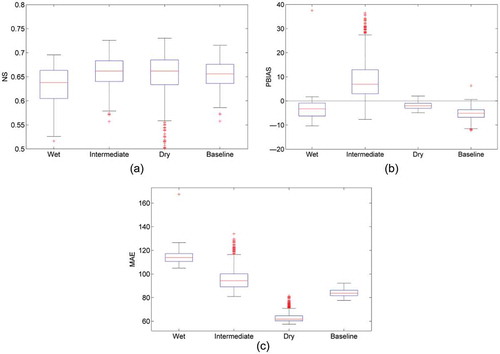
In this section, the general calibration performances of the four calibration periods are analysed. To show the differences between simulated flows and observed flows more clearly, one year from each period is selected randomly and presented in Fig. 5. The results graphically show that the hydrological model simulates the flows quite well. Figure 6 presents the box plots of the Nash-Sutcliffe efficiency coefficient (NS), the overestimation bias in percentage (PBIAS), and the ratio of mean squared error (MAE) in the four calibration periods. On each box, the central mark is the median, the edges of the box are the 25th and 75th percentiles, the whiskers extend to the most extreme data points, and outliers are plotted individually. Nash-Sutcliffe efficiency coefficients distribute much more discretely in the dry sub-period than others, and the dry sub-period has the most outliers. The average values of Nash-Sutcliffe efficiency coefficients of calibration periods are almost the same except for the wet sub-period, which is lower. According to the overestimation bias in percentage, most flows in the intermediate sub-period are overestimated, and almost all flows in the other three sub-periods are underestimated. Compared with the outliers and scattered distribution in the intermediate sub-period, PBIAS in the other three calibration periods are distributed more intensively, which means less uncertainty. According to MAE, the model performance in the dry sub-period is the best. MAE shows that the wet sub-period has the largest errors, and the dry sub-period has the smallest. MAE is the most natural measure of average error magnitude and it seems that all dimensioned evaluations and inter-comparisons of average model performance error should be based on MAE instead of root mean square error (RMSE) (Willmott and Matsuura 2005). Thus, MAE is used in this paper.

Figure 5. Model simulation of the year 1994 in the wet sub-period, 1967 in the intermediate sub-period, 2005 in the dry sub-period and 1980 in the baseline period.

Figure 6. Box plots of (a) NS, (b) PBIAS and (c) MAE values for calibrated simulation sets. These box plots contain n = 981, 1000, 792, 946 simulations in the wet, intermediate and dry sub-periods and the baseline period, respectively. NS: Nash-Sutcliffe efficiency, PBIAS: overestimation bias in percentage and MAE: mean absolute error.

4.3 Validation results

As mentioned in Section 3.2, the aridity indexes of the validation period 1969–1970 corresponding to the climatic condition of HadCM3 and 1978–1979 corresponding to the climatic condition of ECHAM5 are 0.58 and 1.02, respectively, which can be identified as the wet period and the dry period. The k parameter sets (k = 981, 100, 792, 946 from wet, intermediate, dry and baseline calibration sub-periods, respectively) are used to simulate daily flows in the validation periods 1969–1970 and 1978–1979. After validation, the NS, the PBIAS and the ratio of MAE in the validation periods 1969–1970 and 1978–1979 are illustrated respectively in Fig. 7. Almost all the NS coefficients decrease when parameters are transferred from calibration periods (i.e. wet, intermediate, dry and baseline calibration sub-periods) to validation periods. For the validation period 1969–1970, NS coefficients from the parameter set in the wet calibration sub-period are larger compared with the other three parameter sets. While MAE from the parameter sets in the intermediate sub-period, dry sub-period and baseline period increase sharply, MAE from the parameter set in the wet sub-period remain stable. Therefore, for the validation period 1969–1970, the parameter set in the wet sub-period is most favorable.

Figure 7. Comparison of box plots of NS, PBIAS and MAE values between calibrated and validated simulations. The validation periods 1969–1970 and 1978–1979 are corresponding to HadCM3 and ECHAM5, respectively. These box plots contain n = 981, 1000, 792, 946 simulations in the wet, intermediate and dry sub-periods and the baseline period, respectively. NS: Nash-Sutcliffe efficiency, PBIAS: overestimation bias in percentage, and MAE: mean absolute error.

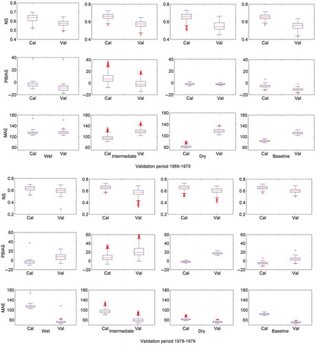
For the validation period 1978–1979, differences between NS coefficients in calibration and validation periods are not so distinct. But biases from the parameter set in the baseline period are the smallest, ranging from −10% to 20%. Mean absolute errors from the parameter set in the baseline period distribute are the smallest and concentrated. Thus, for the validation period 1978–1979, the most suitable parameter set is the parameter set in the baseline period.

4.4 Daily low, medium and high flows during 2011–2040

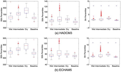
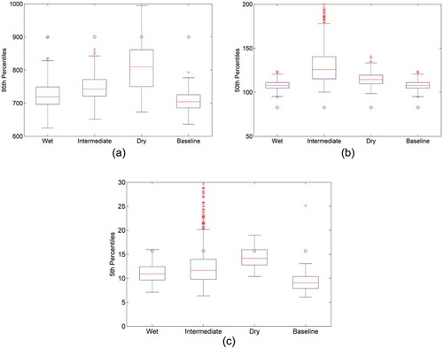
For a comparison of simulated low, medium and high flows in the period 2011–2040 with observed values in the baseline period, 5, 50 and 95 percentiles of flows are calculated (Fig. 8). Overall, the simulated medium flows remain more or less stable regardless of the parameter sets. Low flows tend to decrease a lot in the future using four parameter sets. However, high flows perform inconsistently in different parameter sets. High flows simulated with the parameter set in the intermediate sub-period remain more or less stable, but tend to increase with the parameter set in the dry sub-period and tend to decrease with the parameter set in the wet sub-period and the baseline period. Concerning the uncertainty analysis, the highest uncertainty exists in simulated high flows with the parameter set in the dry sub-period and simulated medium flows with the parameter set in the intermediate sub-period. Simulated low flows show a tight distribution for all parameter sets, with the lowest uncertainty associated with the parameter set in the baseline period.

Figure 8. Comparison of simulated and observed low, median and high daily flows under (a) HadCM3 and (b) ECHAM5. The symbols “o” in the figures represent the values of observed flows. Three percentile values (5, 50 and 95 percentiles) are calculated for simulations, with each parameter set trained in the wet, intermediate and dry sub-periods and the baseline period, respectively. These box plots contain n = 981, 1000, 792, 946 simulations, from left to right.

4.5. Annual changes of runoff during 2011–2040

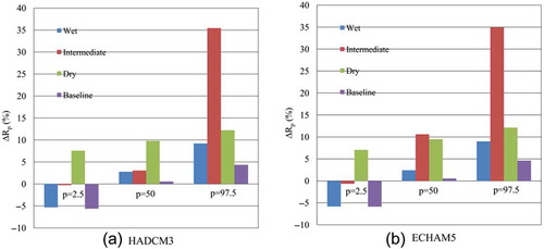
Annual changes are presented in Fig. 9. It turns out that the low annual runoffs tend to increase with the parameters from the dry sub-period, while the low annual runoffs have a decreasing tendency with the other three periods. The changes of 50th percentile values show that average annual runoff has a tendency to increase during 2011–2040 and it tends to increase slightly more under HadCM3 than under ECHAM5, except that the average annual runoff simulated with the parameter set trained in the intermediate sub-period. From the changes of 97.5 percentile values, it can be revealed that the high annual runoffs will increase a lot in the future period 2011–2040. It can be seen that the uncertainty of high annual runoffs are much larger than the low and mean annual runoffs. The results turn out that average annual runoff of 2011–2040 may decrease or increase. Only those simulated with the parameter sets in the dry sub-period show that average annual runoff will consistently increase in the future period. When the uncertainties of different sub-periods are taken into consideration, it shows that the uncertainty of annual runoffs from the intermediate sub-period is the largest, then from the wet sub-period. The uncertainty from the dry sub-period is the smallest.

Figure 9. Annual changes between simulated runoffs in 2011–2040 and observed runoff in 1961–1990 under (a) HadCM3 and (b) ECHAM5.

4.6 Seasonal changes of runoff during 2011–2040

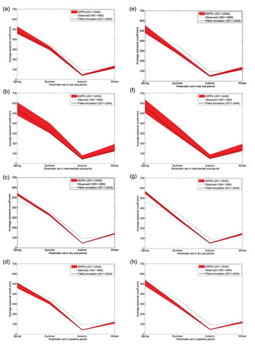
For uncertainty analysis, 95% prediction uncertainty (95PPU) of the simulated seasonal runoffs for 2011–2040 is calculated and illustrated in Fig. 10. In order to compare the k-simulation set approach with the traditional model calibration method of using an individual best fit parameter set approach, seasonal runoff simulated by the individual best fit parameter set is also presented in the figure. In addition, the seasonal runoffs in the future period 2011–2040 and in the baseline period which has observed data are compared to analyse the tendency of the simulated runoff. The results show that the uncertainty of runoffs simulated by the parameter set in the intermediate sub-period is the largest, and simulated by the parameter set in the dry sub-period is the smallest. From the figure, it is known that seasonal runoffs simulated by the individual best fit parameter set in the wet and intermediate sub-periods are comparatively lower, but in dry and baseline periods are higher than most runoffs simulated by the k-simulation set approach. Seasonal runoffs simulated by the individual best fit parameter set in the baseline period are comparatively higher than most simulations by the k-simulation set approach. Apart from these, the largest uncertainty can be observed for spring runoffs and the lowest one for autumn runoffs. Compared with the observed seasonal runoff, it turns out that runoffs in spring and winter tend to increase; however, runoffs in summer and autumn tend to decrease during 2011–2040. Considering the uncertainty of parameters from different sub-periods, it shows that the uncertainty of the parameter from the intermediate sub-period is the largest, while the parameter from the dry sub-period is the smallest. Except the autumn, the uncertainties of seasonal runoff changes in the three other seasons are larger under ECHAM5 than HadCM3.

Figure 10. 95PPU (95% prediction uncertainty) and fitted simulation of seasonal runoff for the period 2011–2040; and seasonal runoff in the period 1961–1990 which has observed data. The four figures ((a), (b), (c), (d)) on the left are under HadCM3, and the right four figures ((e), (f), (g), (h)) are under ECHAM5.

5 Discussion

In this paper, the updated parameter range used in the current iteration is the output of former iteration, and if the updated parameter range goes beyond the initial range, it will be fixed within the initial range manually. But the way of generating new parameter ranges has its limitations. The parameter ranges are proposed to be measured or estimated according to watershed characteristics when data collection is possible (Zhenyao et al. 2013). However, with the constraints of experiments, measured data are not available. For watershed models (e.g. SWAT model), they have both physically-based parameters that can be measured theoretically in the field and empirical parameters that rely only on calibration. It is unrealistic to hope that measured parameter values will be more often used in large-scale watershed models, for the parameters vary spatially. Price et al. (2012) did some different work about the parameter ranges. They extracted 15.9 and 84.1 percentile values from the weighted likelihoods for each parameter and then used these as input ranges for the next iteration. It provides an option, but the main work in the future may expect more advancement from remote sensing techniques and capturing as much spatial variability as possible.

The threshold of Nash-Sutcliffe efficiency coefficients to select flows for uncertainty analysis is 0.5, which is rather subjective, although some works confirm that the threshold is effective (Mishra et al. 2010, Safeeq and Fares 2012). But there is no uniform standard yet for the value of the threshold. In some other SWAT simulation studies, the behavioural threshold of Nash-Sutcliffe efficiency coefficients is 0.6 (Choi and Beven 2007, Looper et al. 2012). In lumped hydrological model applications, the threshold is sometimes 0.7 or 0.8 (Tian et al. 2013). The choice of the threshold will probably affect the uncertainty ranges in the final runoff simulations.

The length of wet, intermediate and dry calibration sub-periods in this study are all four years. Although lots of work had been done to prove that 1- to 5-year calibration period works well to simulate flows with hydrological models (Perrin et al. 2007, Brigode et al. 2013), it seems that it is a little short for the SWAT model, a semi-distributed hydrological model, to get robust parameter sets. After all, in the validation period 1978–1979, the results show that compared with the other three parameter sets, the parameter set trained under the baseline period, which is the longest calibration period, performs best. However, the idea that the longer the calibration period, the more robust the parameter set is not always true, for the parameter set from the wet sub-period acted most appropriately in the validation period 1969–1970 in this study, and the same conclusion can be found in the work done by Perrin et al. (2007).

Nash-Sutcliffe efficiency coefficient is used as the objective function to evaluate calibration efficiency. Figure 11 shows daily low flows simulated in the validation period 1969–1970. NS is expected to emphasize flood peaks during calibration, but it is unexpected in this study to note that simulated high flows in the figure do not match observed high flows better than medium and low flows, for which the reason may be that the calibration periods are not long enough for extreme flows simulation. The simulated 95 percentile flows with the parameter set trained under the dry sub-period match the best with observed 95 percentiles of flow compared with the other three periods. After counting observed daily high flows exceeding 95 percentile flows in the four calibration periods, it is found that the magnitude of observed flows in the dry calibration sub-period is smaller than that in the other three periods, which indicates that parameter sets trained under dry conditions tend to underestimate flows when used to simulate wet conditions. From the PBIAS in Fig. 7, it is known that when the parameter set trained in the wet sub-period is transferred to simulate flows in the dry period (1978–1979), the simulated flows are overestimated. These results are consistent with the conclusions drawn by Coron et al. (2012), who found that the calibration over a wetter (drier) climate than the validation climate leads to an overestimation (underestimation) of the mean simulated runoff.

Figure 11. Comparison of simulated and observed (a) high, (b) median and (c) low flows in the validation period 1969–1970. The symbols “o” in the figures represent the values of observed flows. Three percentile values (5, 50 and 95 percentiles) are calculated for simulations with each parameter set trained in the wet, intermediate and dry sub-periods and the baseline period, respectively. These box plots contain n = 981, 1000, 792, 946 simulations, from left to right.

It can be seen that the results with parameters identified in the intermediate sub-period are completely different from the other three parameter sets. In order to figure out the reasons, the parameter range values of those four calibrated parameter sets are presented in the Table 3. It reveals that ranges of SURLAG, CH_K2 and CN2 from the intermediate sub-period are the largest, which may explain the largest uncertainty of seasonal and annual runoffs with the parameter set from the intermediate sub-period. These three parameters are the most sensitive ones among the 12 parameters, which probably lead to large variations of runoffs.

Table 3. Parameter range values for the SWAT calibrated parameters from three different sub-periods.

	Wet	Intermediate	Dry	Baseline
SURLAG	2.67	3.09	2.80	3.14
CH_K2	42.76	47.33	38.79	39.82
CN2	7.04	9.19	9.08	8.63
ALPHA_BF	0.33	0.32	0.28	0.30
CH_N2	0.08	0.09	0.12	0.08
ESCO	0.44	0.34	0.33	0.49
SOL_AWC()	0.26	0.34	0.09	0.38
CANMX	3.39	3.63	4.83	3.45
SOL_K(1)	22.19	30.16	20.00	32.05
SOL_K(2)	21.00	38.50	30.00	39.10
SOL_Z(1)	842.66	1051.96	9.30	1210.41
SOL_Z(2)	1347.77	1087.56	812.22	1001.00

In this study, only two GCMs are used with one medium emission scenario A1B. The choice of such climate change scenarios is limited to the boundary data for the regional climate model provided by the Met Office, Hadley Climate Centre, UK. Since the focus of this study is on parameter transferability and uncertainty, using limited climate change scenarios is reasonable. However, it must be kept in mind that, in such ways, uncertainty in future simulated flows is underestimated. Besides parameter uncertainty from the hydrological model, in climate change impact analysis, uncertainty originates not only from GCMs, but also emission scenarios, downscaling techniques and hydrological models (Kay et al. 2009, Chiew et al. 2010, Teng et al. 2012, Xu et al. 2013). It is therefore of significance to make a systematic analysis of uncertainties in climate change impact analysis before the results and conclusion can be further used for adaption purposes in water management. Last but not least, it is recommended that multi-objective calibration be promoted instead of single-objective calibration, for multi-objective calibration could capture much more comprehensive hydrological characteristics of the watershed. However, how to combine the objective functions remains a tough task (Kamali et al. 2013).

6 Conclusions

This paper investigated the uncertainty and transferability of parameters in hydrological predictions by identifying three parameter sets from different climatic conditions, which are wet, intermediate and dry conditions. For comparison purposes, another parameter set based on the baseline period from 1961 to 1990 is added, which is sufficiently long to contain wet, intermediate and dry climatic conditions.

It is shown that the parameter set from the wet sub-period performs the best when transferred into wet climate conditions, while the parameter set from the baseline period is the most appropriate when transferred into dry climate conditions. The largest uncertainty of simulated daily high flows in 2011–2040 is from the parameter set trained in the dry sub-period, while that of daily medium and low flows lies in the parameter set from the intermediate calibration sub-period. For annual changes in 2011–2040, the uncertainty with the parameter set from the intermediate sub-period is the largest, followed by the wet sub-period and the dry sub-period. Compared with high and medium flows/runoffs, the uncertainty of low flows/runoffs is much smaller for both simulated daily flows and annual runoffs. For seasonal runoffs, the largest uncertainty is from the intermediate sub-period, while the smallest is from the dry sub-period. Apart from that, the largest uncertainty can be observed for spring runoffs and the lowest one for autumn runoffs.

The k-simulation set approach is proposed in this paper. It was compared with traditional optimization method which uses the single best-fit parameter set. The results show that seasonal runoffs simulated with traditional optimization method in wet and intermediate sub-periods are comparatively lower than most simulations by the k-simulation set approach, while in the baseline period the runoffs are comparatively higher than most simulations by the k-simulation set approach. Therefore, the k-simulation decreases the risks of overestimating or underestimating which is more appropriate for water resources management.

Acknowledgements

National Climate Center of China Meteorological Administration and Zhejiang Hydrological Bureau are greatly acknowledged for providing meteorological and hydrological data in the Qu River basin.

Disclosure statement

No potential conflict of interest was reported by the author(s).

Additional information

Funding

This study is financially supported by the National Natural Science Foundation of China (51379183), Zhejiang Provincial Natural Science Foundation of China (LR14E090001) and the International Science & Technology Cooperation Program of China (2010DFA24320).

References

- Abbaspour, K., 2007. User manual for SWAT-CUP, SWAT calibration and uncertainty analysis programs. Duebendorf: Swiss Federal Institute of Aquatic Science and Technology, Eawag.
- Abbaspour, K.C., et al., 2007. Modelling hydrology and water quality in the pre-alpine/alpine Thur watershed using SWAT. Journal of Hydrology, 333 (2–4), 413–430. doi:10.1016/j.jhydrol.2006.09.014
- Apaydin, H., Anli, A.S., and Ozturk, A., 2006. The temporal transferability of calibrated parameters of a hydrological model. Ecological Modelling, 195 (3–4), 307–317. doi:10.1016/j.ecolmodel.2005.11.032
- Arnold, J.G., et al., 1998. Large area hydrologic modeling and assessment part I: model development1. JAWRA Journal of the American Water Resources Association, 34 (1), 73–89. doi:10.1111/j.1752-1688.1998.tb05961.x
- Bastola, S., Murphy, C., and Sweeney, J., 2011a. Evaluation of the transferability of hydrological model parameters for simulations under changed climatic conditions. Hydrology and Earth System Sciences Discussions, 8 (3), 5891–5915. doi:10.5194/hessd-8-5891-2011
- Bastola, S., Murphy, C., and Sweeney, J., 2011b. The role of hydrological modelling uncertainties in climate change impact assessments of Irish River catchments. Advances in Water Resources, 34 (5), 562–576. doi:10.1016/j.advwatres.2011.01.008
- Beven, K., 2006. A manifesto for the equifinality thesis. Journal of Hydrology, 320 (1–2), 18–36. doi:10.1016/j.jhydrol.2005.07.007
- Beven, K. and Binley, A., 1992. The future of distributed models: model calibration and uncertainty prediction. Hydrological Processes, 6 (3), 279–298. doi:10.1002/hyp.3360060305
- Brigode, P., Oudin, L., and Perrin, C., 2013. Hydrological model parameter instability: A source of additional uncertainty in estimating the hydrological impacts of climate change? Journal of Hydrology, 476, 410–425. doi:10.1016/j.jhydrol.2012.11.012
- Chen, J., et al., 2013. Finding appropriate bias correction methods in downscaling precipitation for hydrologic impact studies over North America. Water Resources Research, 49, 4187–4205. doi:10.1002/wrcr.20331
- Chiew, F.H.S., et al., 2010. Comparison of runoff modelled using rainfall from different downscaling methods for historical and future climates. Journal of Hydrology, 387 (1), 10–23. doi:10.1016/j.jhydrol.2010.03.025
- Choi, H.T. and Beven, K., 2007. Multi-period and multi-criteria model conditioning to reduce prediction uncertainty in an application of TOPMODEL within the GLUE framework. Journal of Hydrology, 332 (3–4), 316–336. doi:10.1016/j.jhydrol.2006.07.012
- Coron, L., et al., 2012. Crash testing hydrological models in contrasted climate conditions: an experiment on 216 Australian catchments. Water Resources Research, 48 (5). doi:10.1029/2011WR011721
- Easton, Z.M., et al., 2008. Re-conceptualizing the soil and water assessment tool (SWAT) model to predict runoff from variable source areas. Journal of Hydrology, 348 (3–4), 279–291. doi:10.1016/j.jhydrol.2007.10.008
- Gan, T.Y. and Burges, S.J., 2006. Assessment of soil-based and calibrated parameters of the Sacramento model and parameter transferability. Journal of Hydrology, 320 (1–2), 117–131. doi:10.1016/j.jhydrol.2005.07.008
- Gordon, C., et al., 2000. The simulation of SST, sea ice extents and ocean heat transports in a version of the Hadley Centre coupled model without flux adjustments. Climate Dynamics, 16 (2–3), 147–168. doi:10.1007/s003820050010
- Gutmann, E.D., et al., 2012. A comparison of statistical and dynamical downscaling of winter precipitation over complex terrain. Journal of Climate, 25 (1), 262–281. doi:10.1175/2011JCLI4109.1
- Hargreaves, G.H. and Samani, Z.A., 1985. Reference crop evapotranspiration from ambient air temperature. American Society of Agricultural Engineers, 1, 96–99.
- Haylock, M.R., et al., 2006. Downscaling heavy precipitation over the United Kingdom: a comparison of dynamical and statistical methods and their future scenarios. International Journal of Climatology, 26 (10), 1397–1415. doi:10.1002/joc.1318
- Hori, M.E. and Ueda, H., 2006. Impact of global warming on the East Asian winter monsoon as revealed by nine coupled atmosphere ocean GCMs. Geophysical Research Letters, 33 (3), 1–4. doi:10.1029/2005GL024961
- Intergovernmental Panel on Climate Change (IPCC), 2007. Climate change 2007: the scientific basis. In: S. Solomon et al., eds. Contribution of Working Group I to the Fourth Assessment Report of the Intergovernmental Panel on Climate Change. New York: Cambridge University Press.
- Kamali, B., Mousavi, S.J., and Abbaspour, K., 2013. Automatic calibration of HEC HMS using single objective and multi objective PSO algorithms. Hydrological Processes, 27 (26), 4028–4042. doi:10.1002/hyp.9510
- Kay, A.L., et al., 2009. Comparison of uncertainty sources for climate change impacts: flood frequency in England. Climatic Change, 92 (1–2), 41–63. doi:10.1007/s10584-008-9471-4
- Kitoh, A. and Uchiyama, T., 2006. Changes in onset and withdrawal of the East Asian summer rainy season by multi-model global warming experiments. Journal of the Meteorological Society of Japan, 84 (2), 247–258. doi:10.2151/jmsj.84.247
- Looper, J.P., Vieux, B.E., and Moreno, M.A., 2012. Assessing the impacts of precipitation bias on distributed hydrologic model calibration and prediction accuracy. Journal of Hydrology, 418–419, 110–122. doi:10.1016/j.jhydrol.2009.09.048
- Maurer, E.P., Brekke, L.D., and Pruitt, T., 2010. Contrasting lumped and distributed hydrology models for estimating climate change impacts on California watersheds1. JAWRA Journal of the American Water Resources Association, 46 (5), 1024–1035. doi:10.1111/j.1752-1688.2010.00473.x
- Min, S-K., Park, E-H., and Kwon, W-T., 2004. Future projections of East Asian climate change from multi-AOGCM ensembles of IPCC SRES scenario simulations. Journal of the Meteorological Society of Japan, 82 (4), 1187–1211. doi:10.2151/jmsj.2004.1187
- Mishra, V., et al., 2010. A regional scale assessment of land use/land cover and climatic changes on water and energy cycle in the upper Midwest United States. International Journal of Climatology, 30 (13), 2025–2044. doi:10.1002/joc.2095
- Mittman, T., et al., 2012. Distributed hydrologic modeling in the suburban landscape: assessing parameter transferability from gauged reference catchments1. JAWRA Journal of the American Water Resources Association, 48 (3), 546–557. doi:10.1111/j.1752-1688.2011.00636.x
- Nash, J. and Sutcliffe, J., 1970. River flow forecasting through conceptual models part I—A discussion of principles. Journal of Hydrology, 10 (3), 282–290. doi:10.1016/0022-1694(70)90255-6
- Perrin, C., et al., 2007. Impact of limited streamflow data on the efficiency and the parameters of rainfall–runoff models. Hydrological Sciences Journal, 52 (1), 131–151. doi:10.1623/hysj.52.1.131
- Piniewski, M., et al., 2013. Effect of modelling scale on the assessment of climate change impact on River runoff. Hydrological Sciences Journal, 58 (4), 737–754. doi:10.1080/02626667.2013.778411
- Price, K., et al., 2012. Tradeoffs among watershed model calibration targets for parameter estimation. Water Resources Research, 48 (10), W10542. doi:10.1029/2012WR012005.
- Ragettli, S. and Pellicciotti, F., 2012. Calibration of a physically based, spatially distributed hydrological model in a glacierized basin: on the use of knowledge from glaciometeorological processes to constrain model parameters. Water Resources Research, 48 (3), W03509. doi:10.1029/2011WR010559
- Roeckner, E., et al., 2003. The atmospheric general circulation model ECHAM5. PART I: model description, Report 349, Max Planck Institute for Meteorology, Hamburg, Germany.
- Safeeq, M. and Fares, A., 2012. Hydrologic response of a Hawaiian watershed to future climate change scenarios. Hydrological Processes, 26 (18), 2745–2764. doi:10.1002/hyp.8328
- Schmidli, J., et al., 2007. Statistical and dynamical downscaling of precipitation: an evaluation and comparison of scenarios for the European Alps. Journal of Geophysical Research: Atmospheres, 112, D04105. doi:10.1029/2005JD007026
- Setegn, S.G., Srinivasan, R., and Dargahi, B., 2008. Hydrological modelling in the Lake Tana Basin, Ethiopia using SWAT model. The Open Hydrology Journal, 2 (1), 49–62. doi:10.2174/1874378100802010049
- Teng, J., et al., 2012. Estimating the relative uncertainties sourced from GCMs and hydrological models in modeling climate change impact on runoff. Journal of Hydrometeorology, 13 (1), 122–139. doi:10.1175/JHM-D-11-058.1
- Themeßl, M.J., Gobiet, A., and Heinrich, G., 2012. Empirical-statistical downscaling and error correction of regional climate models and its impact on the climate change signal. Climatic Change, 112 (2), 449–468. doi:10.1007/s10584-011-0224-4
- Themeßl, M.J., Gobiet, A., and Leuprecht, A., 2011. Empirical-statistical downscaling and error correction of daily precipitation from regional climate models. International Journal of Climatology, 31, 1530–1544. doi:10.1002/joc.2168
- Tian, Y., Xu, Y-P., and Zhang, X-J., 2013. Assessment of climate change impacts on River high flows through comparative use of GR4J, HBV and Xinanjiang Models. Water Resources Management, 27 (8), 2871–2888. doi:10.1007/s11269-013-0321-4
- Van der Linden, S. and Woo, M-K., 2003. Transferability of hydrological model parameters between basins in data-sparse areas, subarctic Canada. Journal of Hydrology, 270 (3–4), 182–194. doi:10.1016/S0022-1694(02)00295-0
- Van Griensven, A., et al., 2006. A global sensitivity analysis tool for the parameters of multi-variable catchment models. Journal of Hydrology, 324 (1–4), 10–23. doi:10.1016/j.jhydrol.2005.09.008
- Vaze, J., et al., 2010. Climate non-stationarity—validity of calibrated rainfall–runoff models for use in climate change studies. Journal of Hydrology, 394 (3–4), 447–457. doi:10.1016/j.jhydrol.2010.09.018
- Wang, X., Melesse, A., and Yang, W., 2006. Influences of potential evapotranspiration estimation methods on SWAT’s hydrologic simulation in a northwestern Minnesota watershed. Transactions of the ASABE, 49 (6), 1755–1771. doi:10.13031/2013.22297
- Wilby, R.L., 2005. Uncertainty in water resource model parameters used for climate change impact assessment. Hydrological Processes, 19 (16), 3201–3219. doi:10.1002/hyp.5819
- Willmott, C.J. and Matsuura, K., 2005. Advantages of the mean absolute error (MAE) over the root mean square error (RMSE) in assessing average model performance. Climate Research, 30 (1), 79–82. doi:10.3354/cr030079
- Xu, Y-P., et al., 2013. Impact of climate change on hydrology of upper reaches of Qiantang River Basin, East China. Journal of Hydrology, 483, 51–60. doi:10.1016/j.jhydrol.2013.01.004
- Xu, Y-P., Zhang, X., and Tian, Y., 2012. Impact of climate change on 24-h design rainfall depth estimation in Qiantang River Basin, East China. Hydrological Processes, 26 (26), 4067–4077. doi:10.1002/hyp.9210
- Zhang, H., et al., 2011. Multi-period calibration of a semi-distributed hydrological model based on hydroclimatic clustering. Advances in Water Resources, 34 (10), 1292–1303. doi:10.1016/j.advwatres.2011.06.005
- Zhang, X., Xu, Y-P., and Fu, G., 2014. Uncertainties in SWAT extreme flow simulation under climate change. Journal of Hydrology, 515, 205–222. doi:10.1016/j.jhydrol.2014.04.064
- Zhenyao, S., Lei, C., and Tao, C., 2013. The influence of parameter distribution uncertainty on hydrological and sediment modeling: a case study of SWAT model applied to the Daning watershed of the Three Gorges Reservoir Region, China. Stochastic Environmental Research and Risk Assessment, 27 (1), 235–251. doi:10.1007/s00477-012-0579-8