
Abstract
We re-evaluated a method to estimate water stress changes as a function of increasing global mean temperature. Trends in the total population under high water stress (defined as when the annual water withdrawal divided by the annual water availability is higher than 0.4) now and in the future (total HWSP) and the population exposed to high water stress in the future but not now (add_HWSP) are dependent on differences in each scenario, not the global mean temperature increase. The ensemble mean of the total HWSP and its ratio for emissions scenarios A1B and B1 are close to constant values and decreased when the global mean temperature increase exceeded 1.9°C and 1.3°C, respectively. If the global mean temperature increase reaches a maximum ensemble-mean value in each scenario, the total HWSP (its ratio) in scenarios A1B, A2 and B1 was about 4.5 billion (0.54), 8.6 billion (0.64) and 4.1 billion (0.49), respectively. We estimated the contributions of climate change to runoff, water withdrawal and population growth on total HWSP and add_HWSP to separate the influences of climate change and socio-economic change. Climate change and socio-economic factors (water withdrawal and population growth) decreased and increased add_HWSP, respectively.
Editor Z.W. Kundzewicz
Résumé
Nous avons réévalué une méthode d’estimation du stress hydrique en fonction de l’augmentation de température moyenne de la planète. Les tendances de la population (PSHE) déjà soumise à un stress hydrique élevé (défini par un rapport du prélèvement annuel d’eau à la disponibilité annuelle en eau supérieur à 0,4), et de la population qui n’y sera qu’à l’avenir exposée (PSHE_suppl) dépendent des différences de chaque scénario, mais pas de l’augmentation de la température moyenne mondiale. La moyenne d’ensemble de la PSHE et sa proportion par rapport à la population totale (PRPT) pour les scénarios d’émission A1B et B1 sont pratiquement constantes et diminuent lorsque l’augmentation de la température moyenne mondiale dépasse respectivement 1,9°C et 1,3°C. Si l’augmentation de la température moyenne mondiale atteint une valeur maximale de la moyenne d’ensemble dans chaque scénario, la PSHE (et sa PRPT) dans les scénarios A1B, A2 et B1, sont respectivement d’environ 4,5 milliards (0,54), 8,6 milliards (0,64) et 4,1 milliards (0,49). Nous avons estimé les effets du changement climatique sur les écoulements et les prélèvements d’eau, et de la croissance de la population sur la PSHE et la PSHE_suppl, pour séparer les effets du changement climatique et des changements socio-économiques. Le changement climatique et les facteurs socio-économiques (prélèvements d’eau et croissance de la population) ont respectivement diminué et augmenté PSHE_suppl.
Key words:
1 BACKGROUND
An evaluation of the impacts induced by climate and socio-economic change is important for understanding climate change in the future, particularly when discussing adaptation plans from a damage scale and cost balance perspective. Parry et al. (Citation2001) and Arnell et al. (Citation2002) evaluated the risks of water shortages, malaria, food and coastal floods as a function of an increase of global mean temperature using a single general circulation model (GCM). According to their results, the number of people affected by a shortage of water will abruptly increase if global mean temperature increases by 1.5–2.0°C from now until 2080. They insisted that we need to reduce emissions to significantly decrease the number of individuals at risk. However, their evaluation of critical climate change threats and water shortage did not account for uncertainty of the GCM output (using only one GCM), the impact of anthropogenic changes and water withdrawal as a proportion of water availability. The fourth report of the Intergovernmental Panel on Climate Change (IPCC Citation2007) illustrates the impact of each sector as a function of global mean temperature. A water stress evaluation by global mean temperature could also help set the target for reduction in emissions. However, this evaluation of water stress as a function of global mean temperature has not been illustrated within the uncertainty of the evaluations made so far.
Shen et al. (Citation2014) investigated world water resource stress in the Special Report on Emission Scenarios (SRES; IPCC Citation2000) and evaluated the number of people living in highly water-stressed basins. The highly water-stressed population (HWSP) included approximately 2.53 billion people. This number will increase in the future and possibly double by 2050 according to SRES scenarios A1B, A2 and B1. They determined that population growth and socio-economic development are the major causes of increasing stress on world water resources. Climate warming could mitigate world water stress to a limited extent. However, these results were a function of time not global mean temperature. An assessment of HWSP considering global mean temperature and socio-economic development is necessary, because it aids understanding of how much we should reduce CO2 emissions. Recently, Parish et al. (Citation2012) developed a simple method to estimate the water stresses based on changes in climate and population. Their study provided a framework for combining climate model and population data into a form that may be useful for water planning. This kind of simple method is useful in the case of only a limited statistical dataset, but in their study, we can point out the lack of evaluation of the uncertainty of the GCM itself, consideration of economic changes, and viewpoint of the relationship between water stress and global mean temperature increase from current.
The purpose of this study was to re-evaluate the method for estimating water stress dependence on the global mean temperature increase and the contributions of climate change, population growth and economic growth to HWSP. This re-evaluation could be helpful in supporting policy-making decisions. We present a multi-GCM analysis of the global and regional populations living in highly water-stressed basins as a function of global mean temperature using socio-economic data, multi-model GCM outputs and multiple scenarios.
2 DATA SOURCES AND METHODOLOGY
Various sources of socio-economic data are utilized for estimation of the geographical distribution of current water withdrawal and the projection of future change. Country-based statistical data of water withdrawal by each water-use sector from AQUASTAT (Citation2012), a global database on water use, were used to estimate the geographical distribution of current water withdrawals. An irrigation area map (Döll and Siebert Citation2002) and our state-of-the-art gridded urban/rural population dataset, which was generated by referencing the Oak Ridge National Laboratory’s (ORNL) Landscan 2002 dataset, the UN’s urban/rural ratio data for 2003 and a global land-cover dataset based on MODIS satellite data (Bengtsson et al. Citation2007), were utilized.
For future projections, SRES-based datasets, such as those for population, GDP, total energy and electricity consumption/production, and other data from various organizations were used. For the population data, we used our 0.5o gridded dataset (Bengtsson et al. Citation2007) based on country-level population data (CIESIN Citation2002a, Citation2002b), downscaled from SRES regional forecasts. The country-based GDP dataset downscaled from regional forecasts of the SRES, was also provided by CIESIN (Citation2002c). The GDP and industrial GDP percentage data for each country reported in the World Development Indicators 2005 (World Bank Citation2005), country-based statistical data on population, and electricity and total energy consumption for 1980–2000 were used to develop the method for estimating future industrial water withdrawals.
The future simulation results of six GCMs—NASA/Goddard Institute for Space (USA), CCSR/NIES (Japan), Max Planck Institute for Meteorology (Germany), MRI (Japan), NCAR (USA) and Hadley Centre for Climate Prediction and Research, MetOffice (UK); see —based on the three IPCC SRES scenarios (A1B, A2 and B1) were used to analyse the availability of freshwater resources under climate warming. For the estimation of the water resources in the future, we used the river discharge obtained using Total Runoff Integrating Pathways (TRIP; Oki and Sud Citation1998) data, which was calculated by six GCMs based on the different SRES scenarios. For estimation of the present river discharge, the Second Global Soil Wetness Project (GSWP2; Dirmeyer et al. Citation2006) runoff data were used.
Table 1 Description of climate forecasting data used for the water resources analysis. Numbers shown in parentheses are the approximate distance at the Equator between grid cells in km.
Water withdrawals (agriculture water, domestic water and industrial water) were predicted as follows:
We estimated future agricultural water withdrawal based on increases in irrigated land use and change in irrigation intensity (annual irrigation quantity per unit area) for each country according to Shen et al. (Citation2008). Increase in irrigated land was found to be linearly correlated with population growth during the period 1960–2000 (Shen et al. Citation2008, Figure 4). This growth will be limited by cropland availability, which we assume cannot increase. However, the increase in irrigated fields will also be restrained by population growth. Non-agricultural land requirements, such as land for residential, traffic, environmental and recreational uses, will definitely increase with population growth. Therefore, we set a limiting factor to each grid by considering the limitation of arable land and necessary non-agricultural land requirement due to population density change. In this study, we set the minimum necessary land for non-agricultural purposes as 150 m2 per capita. Irrigation water diversion efficiency and irrigation intensity (in mm/ha) have opposing effects on water withdrawal for agricultural use. Here, we simply assume that the integrated result of these two factors will not change.
For prediction of industrial water demand, we assumed that the factor of change of the quantity of industrial water demand was a combination of changes of industrial scale and water use efficiency, and then predicted the quantity of future industrial water demand by multiplying the current industrial water demand by the growth rate of industrial scale relative to the present, and the coefficient of water use efficiency improvement. The growth rate of industrial scale of a country is usually measured by the industrial GDP (gross domestic product). However, the socio-economic scenarios set by SRES do not include detailed prediction of the GDP share of the industrial sector. Instead, Shen et al. (Citation2008) found that electricity consumption has a significant linear correlation with industrial GDP and can be used as a measure of industrial scale. We adopted electricity consumption growth as the indicator of change of industrial scale. However, industrial water use does not necessarily increase linearly with industrial growth (e.g. Jia et al. Citation2006). Shen et al. (Citation2008) set a coefficient to account for the effect of industrial restructuring and water use efficiency improvements. They assumed that industrial restructuring and water use efficiency change are reasonably reflected by the change in energy consumption intensity. So, they set the change rate of energy consumption intensity as the indicator for the restructuring and improvement rate of water use efficiency. The industrial water withdrawal of each country was distributed from the national withdrawal data obtained from the AQUASTAT (online database, 2000) used by the FAO (Food and Agriculture Organization of the United Nations). First, we assumed the spatial distribution of industrial water withdrawal is proportional to the urban population within that country; then, the industrial withdrawal was distributed spatially to each grid in proportion to the urban population, initially at a fine spatial resolution of 3-min, then aggregated to 0.5° grids.
We applied a future GDP prediction to the approximation curve of the relationship between GDP and current domestic water withdrawal, and then obtained the future domestic water demand according to Shen et al. (Citation2008). Considering the economic development scenarios using GDP per capita, Utsumi (Citation2006) proposed that future domestic water use intensity was projected by population and GDP scenarios. An equation was obtained by investigating the log–log scatterplot of economic level (as GDP per capita) and domestic water withdrawal intensity (m3 capita-1 year-1) of all countries in 1990. Current total quantity of water withdrawal was defined as the quantity of water withdrawal by country in 2000. The quantity of water withdrawal in each country was obtained from AQUASTAT. The agricultural water demand was distributed in each grid with the distribution map of the areas of irrigation farmland (Döll and Siebert Citation2002, version is 2.1). However, the domestic and industrial water demands were distributed in each grid based on with the population distribution map. The calculation of water stress was carried out for every river basin. That is, we regard the annual discharge at the river mouth as the available water resource of a given river basin, and the water withdrawal quantity over the river basin as the water demand on water resources over the river basin.
The global mean temperature outputs of the six GCMs were used to indicate the future global mean temperature change in the world. The future global mean temperature change is calculated by subtracting the present global mean temperature from the future global mean temperature. We also used the runoff (total runoff value) outputs of the six GCMs to estimate the future potential change in water resources supply. Using the same method as Shen et al. (Citation2014), we averaged the 30-year GCM predictions at each time slice to minimize inter-annual variability. The differences from the present time slice of the annual global mean temperature and runoff at 0.5° grids in the 2020s (2010–2039), 2050s (2040–2069) and 2070s (2070–2099), simulated by each GCM, were then treated as the change due to global warming. To obtain the spatial distribution of future runoff, these changes were added to the 10-year mean runoff data of the Global Soil Wetness Project 2 (GSWP2) multi-model products, generated by ensemble mean of 13 land surface models (LSMs) from various worldwide organizations using a unique forcing dataset (see Diemeyer et al. Citation2006). Recently, some multi-model products have become available. To compare the results of Shen et al. (Citation2014), we selected the product of GSWP2. We did a simple bias correction named the delta-change approach. First, we calculated the difference between each GCM’s output in a specific future period and the output for 1961–1990; we called this difference CHANGE. Then, we added CHANGE (the differences simulated by each GCM) to the results of GSWP2 to obtain the water availability in the future period.
There are two widely-used water stress indices that can be used to assess the world water resources condition from the viewpoint of water stress. One index is the so-called withdrawal-to-availability ratio, defined as the annual water withdrawal (W) divided by annual water availability (Q) at basin scale, W/Q, where the W is annual water withdrawal by agricultural, industrial and domestic sectors, and Q is annual renewable freshwater resources (e.g. Falkenmark et al. Citation1989, WMO Citation1997, Vörösmarty Citation2000). Usually, the extent of water stress is categorized as no-stress (W/Q ≤ 0.1), low stress (0.1 < W/Q ≤ 0.2), moderate stress (0.2 < W/Q ≤ 0.4), and high stress (W/Q > 0.4). This classification was used by WMO (Citation1997), Vörösmarty et al. (Citation2000), Alcamo et al. (Citation2003, Citation2007), Cosgrove and Rijsberman (Citation2000), Oki et al. (Citation2001), and Alcamo et al. (Citation2007), and the W/Q index has the advantage of reflecting the integrated effects of both the pressure from human society (the demand side) and the hydrological system (the supply side).
Another widely-used index is the water scarcity index, which is defined as per capita water availability (Q/c, annual freshwater resource divided by population at river basin scale, in m3 capita-1 year-1). The water scarcity index Q/c is the inverse of the original Falkenmark water crowding indicator (the number of people sharing one flow unit of blue water, Falkenmark and Rockström Citation2004). We adopt the commonly-used classification of water stress extent for Q/c: no stress (Q/c > 1700 m3 capita-1 year-1), moderate stress (1000 < Q/c < 1700 m3 capita-1 year-1), and high stress (Q/c < 1000 m3 capita-1 year-1). Sometimes, a river basin with Q/c less than 500 m3 capita-1 year-1 is marked as extreme stress. Many studies have used this classification, such as Arnell (Citation1999, Citation2004), Alcamo et al. (Citation2003, Citation2007), UNEP (2004), Oki and Kanae (Citation2006), Alcamo et al. (Citation2007). The advantage of this index is its simplicity, the only relevant parameters are population and water availability. But it cannot reflect other factors influencing the water resources situation, e.g. water use and management technologies.
In this study, we used a water stress index defined as the annual water withdrawal divided by the annual water availability at the basin scale, and called W/Q.
3 TOTAL HWSP AND ADD_HWSP AS A FUNCTION OF GLOBAL MEAN TEMPERATURE INCREASE
Total HWSP and its ratio (the calculated total HWSP divided by global population) in the world were estimated as a function of global mean temperature () and ()). Social elements (population, GDP) were also recalculated as a function of global mean temperature increase (e.g. ) and W/Q distributions in the present and future for each scenario are also shown (). The maximum global mean temperature increase was different for each scenario, because it depended on the predicted global mean temperature from the GCM output for each scenario. So the horizontal error bars were indicated from multi-model GCMs. Uncertainties in a climate model are illustrated with horizontal and vertical error bars by using the multi-model GCMs. In the global assessment, the ensemble-mean increase in total HWSP for Scenario A2 was larger than that for other scenarios, which agreed with the results of Oki and Kanae (Citation2006). Values of the ensemble-mean of total HWSP and its ratio were almost the same for scenarios A1B and B1, and decreased when the global mean temperature increase exceeded 1.9°C and 1.3°C, respectively. However, for Scenario A2, values were higher than for scenarios A1B and B1. This implies that population in the region where the HWSP is already high increases more than where the HWSP is low now. If the global mean temperature increase reaches a maximum ensemble-mean value in each scenario, the total HWSP (its ratio) in scenarios A1B, A2 and B1, is about 4.5 billion (0.54), about 8.6 billion (0.64), and about 4.1 billion (0.49), respectively.
Fig. 1 Plots of (a) the total highly water-stressed population (HWSP), (b) total HWSP ratio and (c) add_HWSP vs the global mean temperature warmer than present in the 2070s. Error bars in (a) and (b) indicate the variability of multi-GCM outputs. Grey shading indicates the curve of Parry et al. (Citation2001). The black dashed line indicates the spline curve connecting the average values in each scenario; the black dashed line indicates the cubic polynomial approximation curve.
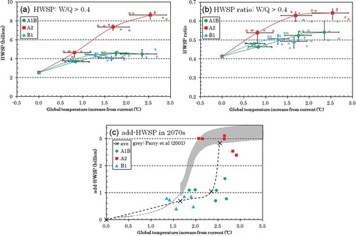
Fig. 2 Plot of population vs global mean temperature anomaly from present. Filled markers indicate the average of multi models in each scenario. Upper and lower open markers indicate the maximum and minimum values for each scenario, respectively. The broken lines indicate the use of fewer than five general circulation models (GCMs).
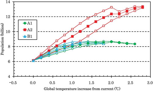
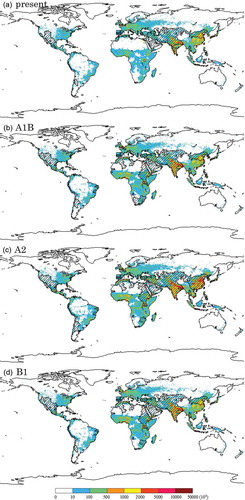
Fig. 3 (a) Spatial distribution of the population and the high W/Q (>0.4) (a) in the present, (b), (c) and (d) for the 2070s for scenarios A1B, A2 and B1, respectively. The colour scale and black hatching indicate population and the high W/Q (>0.4) area, respectively.
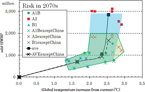
In ) we illustrate add_HWSP relative to add_HWSP derived using the global mean temperature function of Parry et al. (Citation2001), which is the exposed potential high water-stressed population, overlapped on the curve indicated by Parry et al. (Citation2001). The shape of the black dashed and solid lines in is strongly controlled by the high value of add-HWSP in Scenario A2. In Figure 1 of Parry et al. (Citation2001), there is a sigmoidal shape. This difference should be caused by the distribution of the scenarios. When we only see the curve connecting the average value of each scenario (i.e. without uncertainty), a major change occurs around 2.5°C. We might say that the critical point has shifted to a warmer global mean temperature, but the influence of differences between scenarios is dominant, because the distribution of the points can clearly be divided into each scenario and can be explained by the uncertainty of multi-GCMs. To avoid misunderstandings from this kind of analysis, it is necessary to consider using the multi-GCMs. From this analysis, the ratios of the add_HWSP in each country were calculated. Because it was considered that the socio-economic effect in China will be great, we show the add_HWSP both including and excluding China in . The add_HWSP in Scenario A2 only clearly showed a difference of influence of China, which is strongly related to the population increase and economic growth.
Fig. 4 Plot of the highly water-stressed population (add_HWSP) over the world with and without China, vs the global mean temperature warmer than present in the 2070s.
Whether water stress will become better or worse in the future is more useful information than the water stress index value itself. shows the ratio of global population living in regions where water stress becomes worse or better in the future (2070s for Scenario A1) relative to the present, in each bin of the present water stress index (W/Q). For example, the value in the box with horizontal axis from 0.0 to 0.2, and vertical axis is from 0.0 to 0.1, means the ratio of population living in regions where present water stress is 0.0–0.2, and the subtraction of present water stress from that in the 2070s is 0.0–0.1. A positive value from the subtraction (vertical axis) means that the water stress will become worse. In fact, 93.4% of all populations live in a region where the water stress will become worse. However, it would still be unwise to conclude from this result that the change of renewable water freshwater resources by climate change results in worse W/Q. The GCM simulations based on the SRES include not only climate change but also socio-economic change.
Table 2 Percentage of global population living in regions under water stress showing the difference between W/Q (future minus present), in the 2070s for Scenario A1, in each bin of the present water stress index (W/Q).
4 SENSITIVITY ANALYSIS OF CLIMATIC AND SOCIO-ECONOMIC FACTORS ON HWSP
In Section 2, we showed water stress in the future and its change, which implied that the the water stress index included not only the societal change on climate but society impacts. Here, we show the sensitivities of the effects of climate and society on water stress in the future. To indicate the sensitivities of climate change and socio-economic factors for add_HWSP, we estimated add_HWSP in each scenario when each factor (discharge, population and water withdrawal) was set to the present level (). We used the ensemble-mean of outputs of multi-GCMs for input to these estimations. In , the sensitivities of each factor to add_HWSP are shown as the difference between the add_HWSP lines of each fixed factor and the add_HWSP line along each scenario (bold line). The sensitivity of the add_HWSP value to climate change, population, and water withdrawal are indicated.
Fig. 5 Plot of highly water-stressed population (add_HWSP) vs global mean temperature anomaly from present for scenarios: (a) SRES A1B, (b) SRES A2 and (c) B1. The bold line represents the estimation of add_HWSP for each SRES scenario. Q_fixed, W_fixed and P_fixed refer to the estimation of add_HWSP when discharge, water use and population are fixed values, equal to the present level, respectively. If a line is located above the bold line in each scenario, it represents a contribution to a decrease in add_HWSP.
The sensitivities of population and water withdrawal to an increase in add_total HWSP were positive in each scenario. The sensitivity of population to an increase in add_HWSP was similar to the sensitivity of water withdrawal in scenarios A2 and B1. The sensitivity of population to an increase in add_HWSP was about 24% of the sensitivity of water withdrawal. According to population change in scenarios A1B and B1 (Figure 1 of Shen et al. Citation2008), the population is predicted to become constant at around +1.0 to +1.5°C in about 2050 (not shown). However, the priority in scenarios A1B and B1 is the economy and the environment, respectively. The increase in water withdrawal could be restricted by the rapid development and transfer of new technology and energy considering the world environment in Scenario B1. Antithetically, in the case that we think the economy is more important than the environment based on Scenario A1B, the sensitivity of population to an increase of add_HWSP is smaller than the water withdrawal.
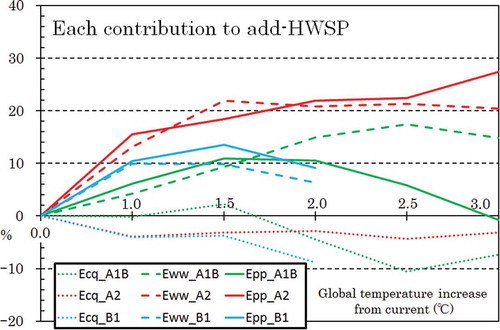
To evaluate the sensitivity to an increase in add_HWSP from each factor objectively, we tried to explain the ratio (contribution) of each factor in each scenario in the 2070s. It is expressed as:
where Ecq, Eww and Epp represent the ratio to an increase in add_HWSP from climate change, water withdrawal and population growth, respectively. The subscripts Q_fixed, W_fixed and P_fixed in equations (1), (2) and (3) refer to the fixed element (discharge, water withdrawal and population, respectively) at the present level. These ratios are shown as explanatory variables in . As shown in , the changing climate acts upon a decrease in the add_HWSP in each scenario. It is clear that the effect of world population growth in Scenario A1B is smaller than that of A2.
Fig. 6 Plot of the sensitivities of changing climate, water withdrawal and population variability for add_HWSP (highly water-stressed population) vs the global mean temperature warmer than present in the 2070s. Blue, green and red lines indicate the contribution ratio to add_HWSP by changing climate, water withdrawal and population, respectively. Solid, dashed and dotted lines represent the values in scenarios A1B, A2 and B1, respectively.
Because we predicted total HWSP and add_HWSP for each country converted from the basin scale, we showed which factor contributes to an increase in the water-stressed population of each country in the future. The spatial distribution of the ratios for each factor in each SRES scenario in the 2070s is shown in . In addition, total HWSP, add_HWSP and the ratio of each sector in each country for each scenario are listed in . Roughly speaking, climate change reduced the add_HWSP. In contrast, the sensitivities to water withdrawal and population growth are dominant. Interestingly, the distribution of the ratio of water withdrawal in the USA, Australia and Kazakhstan contributed to reduce add_HWSP. This feature indicates that water usage efficiency should be sufficiently realized in the future. Additionally, we can say that the climate change-induced discharge reduces the add_HWSP in Russia, India and China, but human activities may make the add_HWSP increase, except for the case of China in SRES Scenario A1B. Also, almost all African countries have similar characteristics to the above. Of course, it is necessary to improve the separation of the effects of population and water withdrawal, but such information, generated for individual countries, should help in policy making for adaptation to climate change using the cooperation between the countries or regions regarding the techniques of effective usage (e.g. saving water, storage of water) and appropriate distribution of water resources.
Fig. 7 Sensitivity of the highly water-stressed population (add_HWSP) in the 2070s to each factor (CC: climate change; WU: water withdrawal; and POP: population growth): (a–c), (d–f), and (g–i) are estimated under scenarios A1B, A2 and B1, respectively. Blue and red indicate contribution to reduction and increase in add_HWSP, respectively.
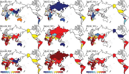
Table 3 List by country of the total highly water-stressed population (HWSP) at present, the highly water-stressed population (add_HWSP), the predicted population, and the contribution ratio of climate change (CC), water withdrawal (WU) and population growth (POP) to add_HWSP under the SRES scenarios A1B, A2 and B1 in the 2070s. Unit of HWSP is million persons and % is percentage of country total population.
5 SUMMARY
We re-evaluated the method for estimating water stress, which depends on a relationship with global mean temperature increase and indicated the uncertainty of the GCM output. The trends in total HWSP and add_HWSP are largely dependent on differences in each SRES emissions scenario, including the socio-economic factors, but not on global mean temperature increase.
We also carried out a sensitivity analysis of climate change, water withdrawal and population growth on the total HWSP and add_HWSP. We concluded the following:
Total HWSP and add_HWSP are shown as a function of global mean temperature increase using the socio-economic data and output of multi-models under several SRES scenarios. These estimations are shown containing the uncertainty of GCM outputs. Interestingly, the ensemble-mean of add_HWSP increased rapidly similar to the result shown in Parry et al. (Citation2001), but the reason for this was due to the differences in socio-economic variance within each scenario and the uncertainty of global mean temperature and runoff of a climate model. Moreover the necessity of using multi-GCMs to avoid such misunderstanding was shown.
The sensitivities of climate change, water withdrawal, and population growth to add_HWSP were evaluated. On global average, the climate change effect on discharge reduces add_HWSP.
Understanding the impct of these sensitivities related to anthropogenic activity are important to avoid high water stress.
In the analysis of this study, we did not carry out the estimation of water stress under SRES Scenario B2, because the main purpose is to re-evaluate the results of Shen et al. (Citation2008) and to show water stress as a function of global mean temperature increase. Given the results that the estimation of water withdrawal under SRES Scenario B2 is similar to that under Scenario A1B (Shen et al. Citation2008), it is probable that the total HWSP and add_HWSP under Scenario B2 will be similar to the results for Scenario A1B.
As mentioned, Parry et al. (Citation2001) and Arnell et al. (Citation2002) evaluated the risks of water shortage. Their studies used a single GCM model and did not consider human activities, except for population change and river basin scale. Arnell et al. (Citation2011) assessed the implications of climate policy for exposure to water resources stresses; they used four GCMs for the climate patterns and indicated the uncertainties of the GCMs itself. Two emissions scenarios were prepared and the ADAM socio-economic scenarios (Bouwman et al. Citation2006) were utilized. An impact on water resources was shown, but their results were not plotted as a function of increasing global mean temperature. Recently, Parish et al. (Citation2012) developed a simple method to estimate the water stresses relating to the combination of population change and water demand, but the uncertainty of simulation was not shown. In the present study, the advantage is that we indicate the uncertainties of GCMs and how in the future some social and economic factors affect the risk of water resources shortage.
Our method is simple and it is impossible to completely separate the contribution of population and water withdrawal to the total HWSP and the add_HWSP, because we consider the population variability when we estimate the water withdrawal. Even the agriculture withdrawal includes the population variability when we estimate the future irrigation area (Shen et al. Citation2008). To separate the contribution of human impacts, it is necessary to improve our method, and a socio-economic model may be useful.
We have only considered annual values, and not the seasonal variability of total HWSP and add_HWSP. We need to focus on seasonal changes, because river discharge and water withdrawal, particularly agricultural withdrawal, vary seasonally. A water-stress assessment considering seasonal variability has been conducted in some other studies (e.g. Hanasaki et al. Citation2008a, Citation2008b, van Beek et al. Citation2011, Wada et al. Citation2011), but an estimate of water stress in the future using the multi-GCM has not yet been conducted. The future task is to calculate total HWSP and add_HWSP using multi-GCM and several scenarios on not only a monthly scale but also with indicators for each grid cell rather than at the basin scale or country scale. Moreover, human activity, such as dam operations, should also be considered for this kind of water-stress assessment. Additionally, we must consider the evolution of technological improvements to human water security (Vörösmarty et al. Citation2010).
The purposes of this study were to re-evaluate the method for estimating water stress dependence on a global mean temperature increase and to evaluate the contribution of socio-economic and climate changes. The results suggest that socio-economic changes contribute to water resources, that society should improve its abilities of adaptation for climate change using the cooperation between the countries and regions and the development of appropriate distribution of water resources, and that we should closely observe changes in socio-economic situations in the future.
Acknowledgements
We thank two anonymous reviewers and the editor for their useful comments. This study was based on the results of projects ‘S-5’ and ‘S-10’, research topics of the Global Environment Research Fund (GERF) of the Ministry of the Environment of Japan. All of the GCM outputs were provided by the Program for Climate Model Diagnosis and Intercomparison (PCMDI).
Related Research Data
REFERENCES
- Alcamo, J., et al., 2003. Global estimates of water withdrawals and availability under current and future ‘business-as-usual’ conditions. Hydrological Sciences Journal, 48 (3), 339–348. doi:10.1623/hysj.48.3.339.45278.
- Alcamo, J., Flörke, M., and Märker, M., 2007. Future long-term changes in global water resources driven by socio-economic and climatic changes. Hydrological Sciences Journal, 52 (2), 247–275. doi:10.1623/hysj.52.2.247.
- AQUASTAT, 2012. FAO’s information system on water and agriculture [online]. FAO. Available from: http://www.fao.org/nr/water/aquastat/main/index.stm [Accessed 20 October 2012].
- Arnell, N.W., 1999. Climate change and global water resources. Environmental Change, 9, S31–S49.
- Arnell, N.W., 2004. Climate change and global water resources: SRES emissions and socio-economic scenarios. Global Environmental Change, 14, 31–52.
- Arnell, N.W., et al., 2002. The consequences of CO2 stabilization for the impacts of climate change. Climatic Change, 53, 413–446. doi:10.1023/A:1015277014327.
- Arnell, N.W., van Vuuren, D.P., and Isaac, M., 2011. The implications of climate policy for the impacts of climate change on global water resources. Global Environmental Change, 21 (2), 592–603. doi:10.1016/j.gloenvcha.2011.01.015.
- Bengtsson, M., Shen, Y., and Oki, T., 2007. A SRES-based gridded global population dataset for 1990–2100. Population and Environment, 28, 113–131. doi:10.1007/s11111-007-0035-8.
- Bouwman, A.F., Kram, T., and Klein Goldewijk, K. 2006. Integrated modelling of global environmental change. An overview of IMAGE 2.4. Netherlands Environmental Assessment Agency, Bilthoven.
- CIESIN (Center for International Earth Science Information Network), 2002a. Country-level population and downscaled projections based on the B2 scenario, 1990–2100 [online]. Palisades, NY: CIESIN, Columbia University. Available from: http://www.ciesin.columbia.edu/datasets/downscaled [Accessed 28 November 2005].
- CIESIN, 2002b. Country-level population and downscaled projections based on the A1, B1 and A2 scenario, 1990–2100 [online]. Palisades, NY: CIESIN, Columbia University. Available from: http://www.ciesin.columbia.edu/datasets/downscaled [Accessed 28 November 2005].
- CIESIN, 2002c. Country-level GDP and downscaled projections based on the SRES A1, A2, B1, and B2 marker scenarios, 1990–2100 [online]. Palisades, NY: CIESIN, Columbia University. Available from: http://www.ciesin.columbia.edu/datasets/downscaled [Accessed 28 November 2005].
- Cosgrove, W. and Rijsberman, F.R., 2000. World water vision: making water everybody’s business. Earthscan Publications, London: World Water Council, 108 pp.
- Dirmeyer, P.A., et al., 2006. The Second Global Soil Wetness Project (GSWP-2): multi-model analysis and implications for our perception of the land surface. Bulletin of the American Meteorological Society, 87, 1381–1397. doi:10.1175/BAMS-87-10-1381.
- Döll, P. and Siebert, S., 2002. Global modeling of irrigation water requirements. Water Resources Research, 38, 1–10.
- Falkenmark, M., Jundqvist, L., and Widstrand, C., 1989. Macro-scale water scarcity requires micro-scale approaches: aspects of vulnerability in semi-arid development. Natural Resources Forum, 13, 258–267. doi:10.1111/j.1477-8947.1989.tb00348.x.
- Falkenmark, M. and Rockström, J. 2004. Balancing water for humans and nature. London: Earthscan Publications, 247.
- Hanasaki, N., et al., 2008a. An integrated model for the assessment of global water resources – Part 1: model description and input meteorological forcing. Hydrology and Earth System Sciences, 12, 1007–1025. doi:10.5194/hess-12-1007-2008.
- Hanasaki, N., et al., 2008b. An integrated model for the assessment of global water resources – Part 2: applications and assessments. Hydrology and Earth System Sciences, 12, 1027–1037. doi:10.5194/hess-12-1027-2008.
- IPCC (Intergovernmental Panel on Climate Change), 2000. Special Report on Emissions Scenarios, Intergovernmental Panel on Climate Change, Cambridge University Press, Cambridge.
- IPCC, 2007. In: M.L. Parry, et al., eds. Climate change 2007: impacts, adaptation and vulnerability. Contribution of Working Group II to the Fourth Assessment Report of the Intergovernmental Panel on Climate Change. Cambridge: Cambridge University Press.
- Jia, S., et al., 2006. Industrial water use Kuznets curve: evidence from industrialized countries and implications for developing countries. Journal of Water Resources Planning and Management, 132 (3), 183–191.
- Oki, T., et al., 2001. Global assessment of current water resources using total runoff integrating pathways. Hydrological Sciences Journal, 46, 983–995. doi:10.1080/02626660109492890.
- Oki, T. and Kanae, S., 2006. Global hydrological cycles and world water resources. Science, 313, 1068–1072. doi:10.1126/science.1128845.
- Oki, T. and Sud, Y.C., 1998. Design of Total Runoff Integrating Pathways (TRIP) – a global river channel network. Earth Interactions, 2, 1–37. doi:10.1175/1087-3562(1998)002<0001:DOTRIP>2.3.CO;2.
- Parish, E.S., et al., 2012. Estimating future global per capita water availability based on changes in climate and population. Computers & Geosciences, 42, 79–86. doi:10.1016/j.cageo.2012.01.019.
- Parry, M., et al., 2001. Millions at risk: defining critical climate change threats and targets. Global Environmental Change, 11 (3), 181–183. doi:10.1016/S0959-3780(01)00011-5.
- Shen, Y., et al., 2008. Projection of future world water resources under SRES scenarios: water withdrawal. Hydrological Sciences Journal, 53 (1), 11–33. doi:10.1623/hysj.53.1.11.
- Shen, Y., et al., 2014 Projection of future world water resources under SRES scenarios: an integrated assessment. Hydrological Science Journal, 59 (10), 1775–1793. doi:10.1080/02626667.2013.862338.
- Utsumi, N., 2006. Global assessment on the future water demand and supply based on SRES scenario. Graduation Thesis. The University of Tokyo, Tokyo, Japan (in Japanese).
- van Beek, L.P.H., Wada, Y., and Bierkens, M.F.P., 2011. Global monthly water stress: 1. Water balance and water availability. Water Resources Research, 47, W07517. doi:10.1029/2010WR009791.
- Vörösmarty, C.J., et al., 2000. Global water resources: vulnerability from climate change and population growth. Science, 289, 284–288. doi:10.1126/science.289.5477.284.
- Vörösmarty, C.J., et al., 2010. Global threats to human water security and river biodiversity. Nature, 467, 555–561. doi:10.1038/nature09440.
- Wada, Y., et al., 2011. Global monthly water stress: 2. Water demand and severity of water stress. Water Resources Research, 47, W07518. doi:10.1029/2010WR009792.
- WMO (World Meteorological Organization), 1997. A comprehensive assessment of the freshwater resources of the world. Geneva: WMO.
- World Bank, 2005. World development indicators 2005 (CD-ROM). Washington, DC: The World Bank.