Testing different cross-section spacing in 1D hydraulic modelling: a case study on Johor River, Malaysia

Abstract

Cross-section data are essential to describe the topography of rivers and floodplain areas and support flood propagation and inundation modelling. To date, there are only a few guidelines available to assist hydraulic modellers in determining the required quantity and location of cross-sections. The aim of this paper is to investigate the impact of cross-section spacing on the results of hydraulic models. To this end, four hydraulic models were built using the HEC-RAS model code and four different numbers of cross-sections. The geometric data were extracted from a high-resolution digital elevation model (LiDAR DEM) of a 30-km reach of the Johor River in Malaysia. These hydraulic models were then compared using flood water levels recorded at two stream gauging stations during two recent flood events. The independent calibration and validation of the models allowed the evaluation of a set of equations proposed in the literature for determining the distance between cross-sections for hydraulic modelling.

Editor D. Koutsoyiannis; Associate editor I. Nalbantis

Résumé

Les données de section en travers sont indispensables pour décrire la topographie des rivières et des zones inondables, et permettre la modélisation de la propagation des crues et celle des inondations. A ce jour, peu de préconisations sont disponibles pour aider les modélisateurs hydrauliciens à déterminer la quantité requise et l’emplacement des sections en travers. Le but de cette étude est de déterminer l’impact de l’espacement entre sections en travers sur les résultats des modèles hydrauliques. A cette fin, quatre modèles hydrauliques ont été construits en utilisant le code du modèle HEC-RAS et quatre nombres de sections en travers. Les données géométriques ont été extraites d’un modèle numérique de terrain à haute résolution (MNT LiDAR) d’un tronçon de 30 km de la rivière Johor en Malaisie. Ces modèles hydrauliques ont ensuite été comparées en utilisant les niveaux d’eau en crue enregistrés à deux stations de jaugeage au cours de deux événements de crue récents. Le calage et la validation indépendants des modèles ont permis d’évaluer un ensemble d’équations proposées dans la littérature pour déterminer la distance entre sections en travers en modélisation hydraulique.

Key words:

• hydraulic modelling
• topographical input
• cross-sections
• LiDAR

Mots clefs:

• modélisation hydraulique
• entrée topographique
• sections en travers
• LiDAR

1 INTRODUCTION

According to the Emergency Events Database (EM-DAT 2012), more than 3000 flood disasters were reported around the world between 1992 and 2011. Those flood events were estimated to affect more than 2 billion people, and cause some 150 000 fatalities and economic losses of around US$480 billion. Depending on the societal context (Berz 2000), flood disasters may lead to damage to infrastructure and loss of human lives (Di Baldassarre et al. 2010). A possible way to reduce the impact of flood disasters is the mapping of flood-prone areas to raise risk awareness and support sustainable land-use planning and urban development (Horritt et al. 2007). Flood mapping is also a useful source of information in rescue and relief missions. In 2007, the European Union (EU) has adopted Directive 2007/60/EC, known as the Flood Directive, with the main objective of reducing and managing flood risk. To this end, all the Member States needed to prepare flood hazard and risk maps by the end of 2013 (van Alphen et al. 2009).

Despite the development of a plethora of two-dimensional (2D) hydraulic models (e.g. Franques and Yannitell 1974, Cunge 1975, Horrit and Bates 2002, Horritt et al. 2006, Tayefi et al. 2007, Cook and Merwadee 2009, Castellarin et al. 2011), one-dimensional (1D) hydraulic models remain widely used for flood risk studies (Baptist et al. 2004, Hooijer et al. 2004, Di Baldassarre et al. 2009). A number of studies have shown that the performance of a 1D model is often very close to that of a 2D model provided that the topography of the river and floodplain is properly represented (e.g. Horrit and Bates 2002, Castellarin et al. 2009, Cook and Merwadee 2009).

In terms of topographic data, 1D modelling requires a certain number of cross-sections to represent the river channel and its surrounding topography (Cook and Merwadee 2009). However, only a few guidelines are available to assist the modeller in determining the location and/or spacing between the cross-sections (Samuels 1990, 1995, Castellarin et al. 2009, Fewtrell et al. 2011). Common sense suggests that locating a river cross-section at every river bend and upstream/downstream of every structure across the river may produce better results. But, having cross-section data at finer spacing, such as at every river meander (i.e. river bend) and upstream/downstream of structures (e.g. bridges) will increase the cost of the topographic surveys. Samuels (1990) recommended certain guidelines for the selection of cross-section locations for 1D hydraulic models. These guidelines were based on a combination of common sense, practical experience and mathematical equations. They guidelines aimed to provide a correct reproduction of the backwater effects and an accurate representation of the physical waves. In general, Samuels (1990) emphasised includion of the following locations for river cross-sections:

1. at both ends of the river reach (upstream and downstream of the reach);

2. at the upstream/downstream of river structures (i.e. bridges or weirs);

3. at all discharge and water level stations along the reach; and

4. at sites that are important to the modeller.

In addition to these ‘essential’ cross-sections, Samuels (1990) recommended the following equations for determining the spacing of the cross-sections:

(1)

where ∆x is the spacing between two cross-sections; B is bankfull surface width of the main channel and k is constant (with the recommended range between 10 and 20).

For an appropriate estimation of backwater effects in subcritical flow, Samuels (1990) suggested:

(2a)

or, if Froude number, Fr = 0,

(2b)

where D is bankfull depth of flow, and s is the main channel slope. Over this length, the backwater upstream of a control (as well other disturbance) decays to less than 0.1 of the original value.

For the unsteady flow condition, an additional equation was suggested where two types of wave might be considered: the flood wave and the tide wave propagating along an estuary:

(3)

where c is the propagation speed of wave; T is the period of wave and N_gp is the number of grid points (varies from 30 to 50).

Finally, the minimum spacing between the cross-sections can be determined due to the influence of the rounding error as follows:

(4)

where q represents the number of decimal digits precision, d is the digits lost due to cancellation of the leading digits of the stage values; s is average surface slope and ε_s is the relative error on surface slope. However, it was noted that, these guidelines were based on the conditions of rivers in the UK.

To test the optimal cross-sectional spacing in 1D hydrodynamic models, Castellarin et al. (2009) presented two case studies in the UK and Italy. Their main objective was to evaluate the efficiency of the 1D model by adopting some of the guidelines and equations recommended by Samuels (1990). As a result, for both selected river reaches, the inaccuracy of the model in terms of mean absolute error was found to increase as the spacing between the cross-sections increases. However, differences between the models were found to be relatively small (less than 0.10 m) and within the accuracy of computational hydraulic models (Samuels 1995, Di Baldassarre and Claps 2011). Castellarin et al. (2009) concluded that, while the minimum spacing of cross-section adopted through the equations (2) and (3) was appropriate for describing the hydraulic behaviour of the river reaches being studied, it was inadequate when the hydraulic models are to be used for designing flood mitigation structures. The main limitation of the study by Castellarin et al. (2009) was that numerical results were not compared against observations. Instead, the results from the hydraulic model with the highest number of cross-sections were used as a benchmark/reference.

Cook and Merwadee (2009) developed 1D hydraulic modelling for two selected river reaches in the USA and highlighted that the simulated flood extent (i.e. inundated area) becomes larger as the number of cross-section increases. Nevertheless, the effects were localized by omitting the structural details (as too much may give a misrepresentation of flooding around the structure). Such action will not affect the overall inundation extent over a reach. In the experiment, the authors also stressed that the increase or decrease of the inundation area were not only influenced by the series of cross-sections used, but also by the widths of the cross-sections.

More recently, Akbari and Barati (2012) investigated the effects of varying time and space steps on model performance in terms of the Nash-Sutcliffe criterion, through numerical tests. Their study showed that the effects of space steps on flood propagation results are less significant than the effects of time steps.

This paper aims to explore the impact of cross-section spacing by using real-world observations. The performance of different 1D hydraulic models based on different cross-section spacing is evaluated (for the first time) using independent calibration and validation data of flood water level observations.

2 STUDY AREA AND DATA

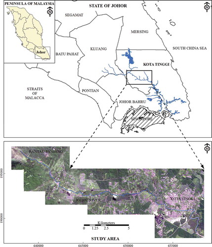
The test site is a 30-km reach of the Johor River between Rantau Panjang River station and 5 km downstream of Kota Tinggi town in the State of Johor, Malaysia (Fig. 1, the river flows from northwest to southeast). The river has an average bed slope of 0.0003 and is characterized by a stable main channel of width 50–250 m, and the bankfull depth of flow ranges between 5.0 and 8.5 m. Most of the floodplain areas are used for agricultural crops and palm plantations. As described by Shafie (2009), this river reach has a meandering channel, with most of the areas showing much sedimentation, ranging from suspended to mixed, as well as bedload sedimentation along the reaches.

Fig. 1 Location and map of the study area: the Johor River, Malaysia.

2.1 Topographic data

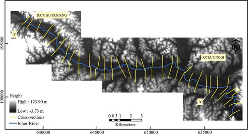
The high-resolution digital elevation model (DEM) of the entire case study area was built by the Department of Irrigation and Drainage, Malaysia (DID) in 2008 using the Light Detection and Ranging (LiDAR) survey method with a horizontal resolution of 1 m. These works were carried out using a Harrier 56/G3 mounted onboard a light aircraft flying at an average height of 700 m with a swath width of approx. 600 m. For the area under water, the topographic survey was carried out through a ground survey method, surveying across the river (average river width range 70–300 m) with approx. 1000 m spacing between the cross-sections. To enable sufficient coverage of the floodplain area in the hydraulic modelling, the DEM from the LiDAR was integrated with the cross-sections from the ground survey (e.g. Castellarin et al. 2009) (Fig. 2).

Fig. 2 Topography of the Johor River, Malaysia, showing reference cross-sections at points X and Y.

2.2 Model description

The HEC-RAS modelling system, developed by the Hydrologic Engineering Center (HEC) of the US Army Corps of Engineers (USACE 2010) was used in this study. The HEC-RAS is a 1D model code that can handle both steady and unsteady flow conditions. For unsteady conditions it solves the full St Venant equations using an implicit finite difference scheme, by means of a solver adapted from the UNET model by Barkau (1997). All simulations in this study were run under unsteady conditions.

To run such simulations using HEC-RAS, the data required include: cross-sections, Manning’s n roughness coefficients, and (upstream and downstream) boundary conditions. The observed flow hydrograph at the upstream end and the normal depth at the downstream end of the river reach were used to define the model boundary conditions. All data required in this hydraulic modelling were obtained from the Department of Irrigation and Drainage, Malaysia (DID).

For the floodplain delineation process, HEC-RAS output was exported to HEC-GeoRAS, an extension for use with the ArcView GIS. The HEC-GeoRAS was developed jointly by the HEC and the Environmental System Research Institute (ESRI), and is specifically intended to assist users with limited GIS experience, especially in processing geospatial data for use with the output from HEC-RAS. The HEC-GeoRAS allows users to create the required geometric data from an existing digital terrain model (DTM) and complementary datasets to run the HEC-RAS model. The delineation process is started by creating a water surface TIN (triangulated irregular network) using the water surface elevation data of each cross-section. Then, the surface TIN is intersected with a bounded polygon to specify that only the area as modelled by HEC-RAS is inundated. The floodplain is then delineated by water surface grids covering the specified area within the bounding polygon. At the same time, the water depth grid is created by subtracting the rasterized water surface TIN and terrain TIN. The water surface between the cross-sections is approximated via linear interpolation.

3 METHODOLOGY

3.1 Cross-section spacing

For this study, four hydraulic models of the Johor River with different spacing of cross-sections were developed: Jhr 1, Jhr 2, Jhr 3 and Jhr 4 (Table 1). All models include the reference cross-section at points X and Y (Fig. 2), as well as the upper and lower cross-section used for the upstream and downstream boundary conditions (see Fig. 3). The cross-sections were derived by integrating the ground survey of the river channel and LiDAR DEM of the floodplain areas.

Table 1 Details of the geometric configuration for each model for the study reach.

Model code	No. of cross-sections	Approx. spacing between cross-sections	Description
Jhr 1	32	~1000 m	Modeller’s own judgement
Jhr 2	16	~2000 m	Modeller’s own judgement
Jhr 3	8	~5000 m	Based on equation (2)
Jhr 4	6	~8000 m	Based on equation (3)

Fig. 3 Cross-section configurations for the four hydraulic models.

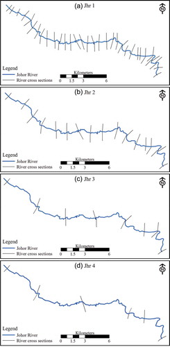
Based on the river characteristics (Table 2) and according to both equations (2) and (3), the minimum spacing between the cross-sections is around 5000 m (Jhr 3) and 8000 m (Jhr 4).

Table 2 Approximate Johor River characteristics.

Bankfull depth of flow, D (m)	Average main channel slope, save	Average Froude number, Frave	Period of wave, T (s)	Propagation speed of wave, c (m/s)
5.0–8.5	0.26–10^-3	0.08–0.35	691 200	0.36

3.2 Hydraulic modelling

Manning’s n roughness coefficient for the river channel was required to perform hydraulic modelling, which ranges from 0.020 to 0.080 m^-1/3 s, while n for floodplains ranges from 0.030 to 0.100 m^-1/3 s (Chow 1959). In order to test the sensitivity of the results to Manning’s n, the models were run using various n values within those ranges. A total of 2000 (500 parameter sets for each of the four models) hydraulic simulations were carried out. In the absence of any knowledge of the prior distribution of the model parameters, a uniform distribution was assumed to select 500 sets of Manning’s n value within these ranges. Apart from the Manning’s n roughness coefficients and cross-section configurations, all other sources of data including the boundary conditions were unchanged for all simulations.

The models were used to simulate two hydrological events: the December 2006 flood (characterized by a peak flow of around 375 m³ s^-1) and the January 2007 flood (about 595 m³ s^-1). These discharge data were measured and recorded at the Rantau Panjang hydrological station.

3.3 Performance of the hydraulic models

The model performance was based on the mean absolute error (MAE) defined as follows:

(5)

where T is the number of steps in the time series; O_t is the observed water level at time t; and S_t is the simulated water level at time t.

For this study, each model was assessed by comparing the simulated flood levels with those observed during the December 2006 and January 2007 flood events at the reference cross-sections X and Y (Fig. 2).

4 RESULTS AND DISCUSSION

In this section we first describe the performance of the 1D hydraulic model for each geometric configuration; then we discuss the influence of geometric configuration on flood inundation in terms of maximum water surface elevation, area of flood extent and flood depth.

4.1 Comparing flood water levels

To investigate the influence of different cross-section spacing on the performance of the 1D models, four models were used (Section 3.1). Figure 4 shows the values of MAE obtained with the four model configurations for simulation of the December 2006 flood (the calibration event).

Fig. 4 Calibration of the four hydraulic models: mean absolute error (MAE) versus the two model parameters for the December 2006 flood event.

Then, the four best fit models (i.e. using the calibrated Manning’s n) were used to simulate the January 2007 flood (validation event). Table 3shows the average MAE of each model for the simulated water levels at cross-sections X and Y. The MAE value for different models did not change significantly as the spacing between the cross-sections was increased from 1000 m to 8000 m.

Table 3 Model results and average MAE obtained at the observation points X and Y (see Fig. 2).

Model code	Calibrated Manning’s coefficients		MAE (m) (validation)
	Channel	Floodplain
Jhr 1	0.050	0.057	0.41
Jhr 2	0.057	0.081	0.52
Jhr 3	0.054	0.081	0.54
Jhr 4	0.055	0.081	0.49

The results of this study, as summarized in Table 3, confirm that the equations recommended by Samuels (1990) provide a proper indication about cross-section spacing. In fact, although the models were derived using different spacing of cross-sections, the difference in MAE is between 0.02 m and 0.13 m.

4.2 Comparing flood water profiles and inundation maps

The results of the hydraulic models can be used to produce flood water profiles (Brandimarte and Di Baldassarre 2012) as well as flood inundation maps (Horritt and Bates 2002) to support flood risk studies. The former are useful for the design of flood protection measures (e.g. dikes and levees), while the latter allow the identification of flood prone areas.

Figure 5 shows the flood water profiles in terms of water surface elevations obtained with the four best fit models. Visual comparison of these four flood water profiles pointed out that, although small differences were found in terms of performance in simulating flood water levels at cross-section X (see Section 4.1), significant differences arise in terms of the spatial distribution of the flood water profiles. This is caused by the absence of topographic information, and therefore geometric input and output, along the river. This outcome suggests that a detailed topographic survey is required when hydraulic modelling is meant to support the design of flood mitigation structures, such as levees (see also Castellarin et al. 2009).

Fig. 5 Flood profile: maximum water surface elevation along the Johor River estimated by the four hydraulic models.

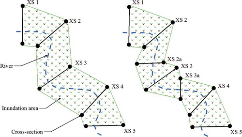
Figure 6 shows the flood inundation maps obtained with the four hydraulic models using the calibrated Manning’s n roughness coefficient, while Table 4  reports the corresponding inundated area. This comparison showed that the error in simulating water elevations at the point X are not significant as differences in MAE are within 0.04 m (Table 4), which is less than the accuracy of LiDAR data (around 0.10 m). In contrast, the resulting flood inundation patterns are rather different (Fig. 6) as the flood extent mapping is strongly affected by the cross-sections used as geometric input to the hydraulic model. In particular, in HEC-GeoRAS the flood inundation extent is generated through a semi-automated process, whereby the topography is subtracted from the water surface elevations. The domain of these inundation maps is created by linearly joining the water surface extent points on each cross-section as depicted in Fig. 7.  Therefore, the resulting inundation extent is related to the placement and the width of the cross-sections as well as definition of the geometry of the river and floodplain, which depends on the detail of the topographic information, i.e. number of cross-sections.

Table 4 Impact of geometric configurations on 1D hydraulic simulation.

Model code	Approx. spacing between cross-sections	MAE at cross-section X (m)	Total inundated area (km^2)
Jhr 1	~1000 m	0.38	24.58
Jhr 2	~2000 m	0.35	23.47
Jhr 3	~5000 m	0.34	22.14
Jhr 4	~8000 m	0.34	18.26

Fig. 6 Effect of different cross-section configurations on flood inundation patterns.

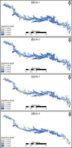
Fig. 7 Effect of cross-section locations on the domain of flood inundation delineation in HEC-GeoRAS.

In summary, this additional analysis shows that if the model is meant to simulate inundation patterns of flood profiles, more cross-sections are needed to capture the spatial heterogeneity of the model domain and the consequent heterogeneity of the model results.

5 CONCLUSIONS

This study investigated the impact of cross-section spacing on the accuracy of 1D hydraulic modelling of floods by testing the few guidelines in the literature via independent calibration and validation exercises.

The performance of the four models (characterized by different cross-section spacing ranging from around 1000 m to around 8000 m; see Table 1) did not show significant differences. For instance, the differences in model performance were between 0.02 and 0.13 m for the validation event of January 2007. This confirms the findings by Castellarin et al. (2009) that the performance of models developed according to Samuels (1990) was as good as that of models with a larger number of cross-sections.

Although model performance at the stream gauging stations X and Y is not significantly affected by model spacing, significant differences in results were obtained in terms of flood extent maps and flood water profiles. This indicates that detailed topographic survey is still needed for the design of flood mitigation structures (e.g. levees) and the identification of flood prone areas.

As a concluding remark, it should be noted that this study did not include the hydraulic structures across the river (e.g. bridges). Furthermore, the releases of discharge from the upstream dam were neglected as well as the discharge from some minor tributaries. Given the specific research objective (i.e. to evaluate the effect of cross-section spacing on model results), we did not include this additional component, which is comprehensively studied by Cook and Merwadee (2009), and Brandimarte and Woldeyes (2013). However, future work will address the issues of determination of the optimal numbers of cross-sections under more complex conditions.

Acknowledgements

The authors would like to acknowledge the Associate Editor and two anonymous reviewers for providing useful and constructive comments. Special thanks to DID, Malaysia Remote Sensing Agency (MACRES), Jurukur Nizam Ali, Jurukur Dr. Abd Majid and MK Survey for providing data used in this study.

Additional information

Funding

This study was supported by a PhD Fellowship awarded to the first author from the Public Service Department, Malaysia and the Department of Irrigation and Drainage, Malaysia (DID).

REFERENCES

- Akbari, G.H. and Barati, R., 2012. Comprehensive analysis of flooding in unmanaged catchments. Proceedings of the ICE – Water Management, 165 (4), 229–238. doi:10.1680/wama.10.00036.
- Baptist, M.J., et al., 2004. Assessment of the effects of cyclic floodplain rejuvenation on flood levels and biodiversity along the Rhine River. River Research and Applications, 20, 285–297. doi:10.1002/rra.778.
- Barkau, R.L., 1997. UNET one-dimensional unsteady flow through a full network of open channels. Davis: User’s Manual, US Army Corps of Engineers, Hydrologic Engineering Center.
- Berz, G., 2000. Flood disasters: lessons from the past-worries for the future. Proceedings of the Institution of Civil Engineers Water & Maritime and Engineering, 142 (1), 3–8.
- Brandimarte, L. and Di Baldassarre, G., 2012. Uncertainty in design flood profiles derived by hydraulic modelling. Hydrology Research, 43 (6), 753–761. doi:10.2166/nh.2011.086.
- Brandimarte, L. and Woldeyes, M.K., 2013. Uncertainty in the estimation of backwater effects at bridge crossings. Hydrological Processes, 27, 1292–1300. doi:10.1002/hyp.9350.
- Castellarin, A., et al., 2009. Optimal cross-sectional spacing in Preissmann scheme 1D hydrodynamic models. Journal of Hydraulic Engineering, 135 (2), 96–105. doi:10.1061/(ASCE)0733-9429(2009)135:2(96).
- Castellarin, A., Di Baldassarre, G., and Brath, A., 2011. Floodplain management strategies for flood attenuation in the River Po. River Research and Applications, 27, 1037–1047. doi:10.1002/rra.1405.
- Chow, V.T., 1959. Open-channel hydraulics. New York: McGraw-Hill.
- Cook, A. and Merwadee, V., 2009. Effect of topographic data, geometric configuration and modeling approach on flood inundation mapping. Journal of Hydrology, 377, 131–142. doi:10.1016/j.jhydrol.2009.08.015.
- Cunge, J.A., 1975. Two dimensional modelling of flood plains. Chapter 17. In: K. Mahmood and V. Yevjevich, eds. Unsteady flow in open channels. Littleton, CO: Water Resources Publications.
- Di Baldassarre, G., Castellarin, A., and Brath, A., 2009. Analysis of the effects of levee heightening on flood propagation: example of the River Po, Italy. Hydrological Sciences Journal, 54 (6), 1007–1017. doi:10.1623/hysj.54.6.1007.
- Di Baldassarre, G. and Claps, P., 2011. A hydraulic study on the applicability of flood rating curves. Hydrology Research, 42 (1), 10–19. doi:10.2166/nh.2010.098.
- Di Baldassarre, G., et al., 2010. Flood fatalities in Africa: from diagnosis to mitigation. Geophysical Research Letters, 37, L22402. doi:10.1029/2010GL045467.
- Emergency Events Database (EM-DAT), 2012. International disaster database. Brussels: Universitè Catholique de Louvain. Available from: http://www.em-dat.net [Accessed September 2012].
- Fewtrell, T.J., et al., 2011. Geometric and structural river channel complexity and the prediction of urban inundation. Hydrological Processes, 25, 3173–3186. doi:10.1002/hyp.8035.
- Franques, J.T. and Yannitell, D.W., 1974. Two-dimensional analysis of backwater at bridges. Journal of the Hydraulics Division, 100 (3), 379–392.
- Hooijer, A., et al., 2004. Towards sustainable flood risk management in the Rhine and Meuse river basins: synopsis of the findings of IRMA-SPONGE. River Research and Applications, 20, 343–357. doi:10.1002/rra.781.
- Horritt, M.S., et al., 2007. Comparing the performance of a 2-D finite element and a 2-D finite volume model of floodplain inundation using airborne SAR imagery. Hydrological Processes, 21, 2745–2759. doi:10.1002/hyp.6486.
- Horritt, M.S. and Bates, P.D., 2002. Evaluation of 1D and 2D numerical models for predicting river flood inundation. Journal of Hydrology, 268 (1–4), 87–99. doi:10.1016/S0022-1694(02)00121-X.
- Horritt, M.S., Bates, P.D., and Mattinson, M.J., 2006. Effects of mesh resolution and topographic representation in 2D finite volume models of shallow water fluvial flow. Journal of Hydrology, 329 (1–2), 306–314. doi:10.1016/j.jhydrol.2006.02.016.
- Samuels, P.G., 1990. Cross-section location in 1-D models. In: White W.R. ed. Proceedings of international conference on river flood hydraulics. Chichester: John Wiley, 339–350.
- Samuels, P.G. 1995. Uncertainty in flood level prediction. In: Proceedings XXVI biannual congress of the IAHR. HYDRA2000, 11–15 September, Thomas Telford, London.
- Shafie, A. 2009. Extreme flood event: a case study on floods of 2006 and 2007 in Johor, Malaysia. In partial fulfilment of the requirements for Degree Master of Science. Fort Collins: Colorado State University.
- Tayefi, V., et al., 2007. A comparison of one- and two-dimensional approaches to modelling flood inundation over complex upland floodplains. Hydrological Processes, 21 (23), 3190–3202. doi:10.1002/hyp.6523.
- USACE, 2010. HEC-RAS river analysis system user’s manual. Version 4.1. Davis, California: Hydrologic Engineering Center.
- van Alphen, J., et al., 2009. Flood risk mapping in Europe, experiences and best practices. Journal of Flood Risk Management, 2, 285–292. doi:10.1111/j.1753-318X.2009.01045.x.