Bridging hydraulic diffusivity from aquifer to particle-size scale: a study on loess sediments from southwest Hungary

Abstract

In situ megascale hydraulic diffusivities (D) of a confined loess aquifer were estimated at various scales (10 ≤ L ≤ 1500 m) by a finite difference model, and laboratory microscale diffusivities of a loess sample by empirical formulas. A scatter plot reveals that D fits to a single power function of L, providing that microscale diffusivities are assigned to L = 1 m and that differences in diffusivity observed between micro- and megascales are assigned to medium heterogeneity appraised by variations in the curvature and slope of natural hydraulic head waves propagating through the aquifer. Subsequently, a general power relationship between D and L is defined where the base and exponent terms stand for the aquifer storage capability under a confined regime of flow, for the microscale hydraulic conductivity and specific yield of loess, and for the changes in curvature and slope of hydraulic head waves relative to values defined at unit scale.

Editor Z.W. Kundzewicz

Résumé

Les diffusivités hydrauliques (D) in situ d’un aquifère captif loessique ont été estimées à différentes méga-échelles (10 ≤ L ≤ 1500 m) par un modèle aux différences finies tout comme les diffusivités de laboratoire l’ont été à la micro-échelle d’un échantillon de loess à partir de formules empiriques. Un diagramme montre que D s’ajuste à une fonction puissance de L à condition que les diffusivités micro-échelle soient affectées à L = 1 m et que les différences de diffusivité observées chez les micro et les méga-échelles soient attribuées à l’hétérogénéité du milieu éstimée par les variations de courbure et de pente des ondes naturelles de charge hydraulique se propageant dans l’aquifère. En conséquence, une relation générale exponentielle entre D et L a été définie, où le terme de base et l’exposant représentent la capacité d’emmagasinement en nappe captive, la conductivité hydraulique et la porosité efficace du loess à micro-échelle, et les changements de courbure et de pente des ondes de charge hydraulique par rapport aux valeurs définies à l’échelle unitaire.

Key words:

• hydraulic diffusivity
• confined aquifer
• loess
• hydraulic head wave
• grain-size distribution
• scale

Mots clefs:

• diffusivité hydraulique
• aquifère captif
• loess
• vague de charge hydraulique
• granulométrie
• échelle

INTRODUCTION

Hydraulic diffusivity is a control parameter of enormous importance in many geological phenomena and engineering problems. For example, hydraulic diffusivity is a key variable in controlling stress release during earthquakes (Talwani 1976, 1997, Talwani et al. 1999, Wibberley 2002, Doan et al. 2006, among others) or basal motion of glaciers overlying deformable beds (Murray 1997, Fischer et al. 2001). It also plays a dominant role in predictions of water content profiles in concrete during wetting and drying conditions, in the context of forecasting the service life of concrete structures (Pradhana et al. 2005, Das and Kondraivendhan 2012, and references therein). But hydrology is the branch of scientific knowledge where hydraulic diffusivity is more extensively used, namely for prediction of natural fluid flow through rock masses (Li 1984, Delépine et al. 2004, Pacheco and Alencoão 2006, Pacheco and Van der Weijden 2012), soil horizons (Appoloni et al. 1990, Chen 1998, Abrisqueta et al. 2006) or aquifer sediments, also known as porous media. The literature on methods for assessing hydraulic diffusivity of porous media aquifers is vast. The most direct method is probably the inverse modelling of hydraulic head fluctuations regulated by groundwater flow equations (Gilmore 1992, Ha et al. 2007, Guo et al. 2010, Pacheco 2013) or spectral relationships (Shih and Lin 2004), because diffusivity is the unknown parameter in these equations or relationships. In line with this method is the analysis of river baseflows (Baloochestani 2008) or more specific algorithms such as the drawdown ratio technique (Neuman and Witherspoon 1972, Leahy 1976). However, because hydraulic diffusivity is a composite parameter, defined as the ratio between transmissivity and storage coefficient, methods based on a separate assessment of these variables were also developed to calculate diffusivity. The most widely used techniques are pumping or slug tests (Trefry and Johnston 1998, Flach et al. 2000, Van der Kamp 2001), but other research tools are also employed, such as geophysical logging, borehole flowmeter tests, direct push methods, or hydraulic tomography (Butler 2005). All the aforementioned approaches determine hydraulic diffusivity under in situ conditions, also referred to as megascale diffusivity, but share a common weakness: they are all costly and time-consuming. In an attempt to circumvent this shortcoming, a group of methods based on laboratory work have gained recognition. Among these techniques are approaches based on empirical relationships between hydraulic parameters and grain-size distributions (Bear 1972, Vuković and Soro 1992, Alyamani and Sen 1993, Odong 2007, among others). These approaches are less costly but measure hydraulic parameters on very small support volumes (hand specimens) and therefore are valid solely at the microscale. In an attempt to bridge diffusivity from the microscale to the megascale, some studies carried out independent evaluation of laboratory results, checking them against values obtained in the field, or wrote empirical relationships between hydraulic parameters and scale (Vienken and Dietrich 2011, Fallico 2014). However, the upscaling of hydraulic diffusivity from the particle-size scale towards the aquifer scale has rarely been discussed from a phenomenological perspective. The purpose of this paper is to fill this gap. To accomplish this goal, a mathematical expression is developed where microscale hydraulic diffusivities, based on the application of empirical formulas to grain-size data, are coupled with megascale diffusivities, based on a finite difference modelling of hydraulic head data performed in a geographic information system at several spatial resolutions. The support volumes in this study range from samples of loess to sectors of a confined loess aquifer, located in southwest Hungary.

STUDY AREA

Location, topography, climate and hydrology

The study region is located in southwest Hungary, in the Szigetvár area, county of Baranya. The topography is hilly in the north and flat in the south of the area, with altitudes ranging from 100 to approximately 400 m a.s.l. (Fig. 1). The climate is classified as Mediterranean, with hot summers and mildly cold snowy winters. The average annual temperature is 9.7°C and average annual precipitation is 600 mm. Rainfall reaches a peak of 80 mm in June, decreasing in subsequent months, with minimum values around 30 mm in the period January–March. In response to recharge by infiltrating precipitation, river flow increases from a minimum of 20 L/s in September to a maximum of 50 L/s in January–February. The lag time between maximum precipitation and maximum river flow is 7 months, which means that infiltration is rather slow (Fig. 2). On a yearly basis, river flow represents only 5.7% of precipitation, indicating a dominance of evapotranspiration in the local water balance.

Fig. 1 Location of the Szigetvár area within the territory of Hungary, showing spatial distribution of topography and lithologic units, and delimitation of a sector where a number of drilled wells were monitored for hydraulic head.

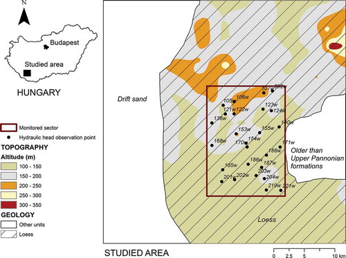
Fig. 2 Seasonal variation of precipitation and river flow data, based on long-term records. The river flow data pertain to the Péli-víz Felsőpél watershed (30.5 km²), measured at a hydrometric station located at the outlet point of this catchment.

Geology

The geology of Szigetvár area is characterized by Upper Pleistocene to Holocene formations. These formations change from drift sand in the western part of the area to loess in the eastern side. In a very small area of the eastern limit, different formations of the western Mecsek mountains were mapped, including Carboniferous granite, Permian sandstone and aleurolite and Miocene gravels or laminated clays (Pacheco and Szocs 2006). In this study, the focus is on the loess area (Fig. 1). There are several studies on the origin and stratigraphy of Hungarian loess (Smalley and Leach 1978, Pécsi 1987, Frechen et al. 1997, Nemecz et al. 2000, Kovács et al. 2011). Loess is wind-blown sediment of silt size formed in periglacial areas during cold and dry periods of the Pleistocene. According to Jámbor (1997), loess was formed during the time span of 1.2 Ma–12 ka. Loess sequences may have transitions to, or alternate with, aeolian sand deposits, and can be interrupted by palaeosol horizons formed during milder interglacial periods. In the Szigetvár area, the loess complex is called the Paks Loess formation (Kovács et al. 2011), in a reference to the most complete exposure located at Paks, a steppe region in the Middle Danube basin, in the Great Hungarian Plain. At this location, the famous ‘Paks brickyard’ has an altitude of approximately 47 m. On average, the Paks Loess formation has a thickness of 25–30 m.

Grain-size distribution and fabric of Hungarian loess and interlayered palaeosols

Several loess and interlayered palaeosol samples were collected by Nemecz et al. (2000) from cleaned walls of loess–palaeosol exposures in the Paks region. After collection, the samples were fractionated using sieving for analysis of grain-size distribution. Table 1 divides averaged samples into the fractions, while Fig. 3 illustrates concomitant grain-size curves. Loess is characterized by a double maximum at the A (clay, <5 μm) and D (coarse silt, 25–40 μm) fractions. Nemecz et al. (2000) noted an accumulation of weathering products such as montmorillonite in the A fraction, and of primary minerals such as quartz, feldspars, micas and dolomite in the D fraction. For this reason, these authors assumed that loess fabric is explained by the formation of steppe soils and not by the mode of dust deposition. The increase in the A fraction of palaeosol, relative to the homologous fraction in loess, is switched in the E fraction. Eventually, this indicates concentration of the most weatherable primary minerals (e.g. plagioclase) in the E fraction. The distribution of particle sizes by the major fractions is (a) loess: silt (51.7%) > clay (27.4%) > sand (20.9%); and (b) palaeosols: silt (51.5%) > clay (41.2%) > sand (7.3%). This corresponds to clay loam and silty clay textures, respectively (Fig. 4).

Fig. 3 Grain-size curves of Hungarian loess and interlayered palaeosols (Paks formation), drawn from the data in Table 1.

Fig. 4 Classification of Hungarian loess and interlayered palaeosols according to texture, based on the grain-size data depicted in Table 1. The textural classification used the USDA soil textural classification.

Table 1 Average grain-size distributions of loess and interlayered palaeosol samples, collected at Paks exposure by Nemecz et al. (2000).

Fraction	Grain size (μm)	Percentage
		Loess	Palaeosol
A	<5	27.4	40.2
B	5–10	5.0	5.5
C	10–20	8.5	8.7
D	20–45	38.1	37.3
E	45–80	18.5	6.8
F	80–160	1.6	0.9
G	160–315	0.5	0.3
H	315–800	0.1	0.0

MATERIALS AND METHODS

Database for hydraulic diffusivity estimation

In this study, hydraulic diffusivity is estimated by a hydrological model and empirical formulas. In the first case, the calculated values will be representative of aquifer-scale diffusivities, also referred to as megascale diffusivities. The second approach calculates estimates of aquifer-scale diffusivities, based on particle-size scale data, a reason why they are also referred to as microscale diffusivities. The estimation of megascale diffusivities relies on the solution of the transient saturated flow equation, which requires prior assessment of hydraulic head data collected from a set of observation points distributed across the study region. The calculation of microscale diffusivities is based on empirical relationships between hydraulic parameters and material granulometry, which involves prior assessment of grain-size distributions.

For the calculation of megascale hydraulic diffusivities, the study used data from the period 1990–1993, when a hydrogeological survey was conducted and funded by the former Geological Institute of Hungary under the project “Geochemical Inspection of Groundwaters”, with the theme “Shallow Groundwater State in South Somogy and Baranya”. During this survey, several drilled wells were observed for hydraulic head on 8 and 16 May 1993. The concomitant hydraulic head records are depicted in Table 2. For the calculation of microscale diffusivities, we used the data given in Table 1.

Table 2 Hydraulic head records of drilled wells represented in Fig. 1. ID: drilled well identification code; X, Y and Z: planimetric and altimetric location coordinates; h: hydraulic head.

ID	Observation date	X (m)	Y (m)	Z (m)	Water depth (m)	h (m)
219w	8 May 1993	407030	342210	123.0	12.4	110.6
201w		399720	343590	125.0	5.9	119.1
202w		401840	343910	132.0	5.4	126.6
204w		406710	344070	168.0	25.0	143.0
203w		405360	344580	139.0	10.5	128.5
171w		409280	349260	138.0	0.6	137.4
170w		403880	349270	137.0	2.0	135.0
168w		398120	349530	164.0	1.6	162.4
154w		403710	349890	150.0	10.1	139.9
153w		402090	351430	204.0	55.3	148.7
136w		398110	353220	201.0	2.7	198.3
106w		401780	356710	223.0	25.2	197.8
221w	16 May 1993	409390	342140	124.0	1.2	122.8
185w		399890	345530	127.0	14.4	112.6
187w		406250	345920	142.5	2.2	140.3
186w		404050	346440	133.0	23.6	109.4
188w		407040	347930	129.0	22.2	106.8
155w		405940	351620	160.0	12.7	147.3
140w		409130	352560	132.0	1.6	130.4
121w		400310	354690	142.0	7.9	134.1
122w		401750	354710	212.0	1.6	210.4
124w		407860	355220	175.0	11.9	163.1
123w		406480	355470	138.0	2.8	135.2
105w		399960	356120	145.0	5.3	139.7
107w		406610	358150	217.0	30.5	186.5
092w		408030	358470	182.0	12.3	169.7

Estimation of megascale hydraulic diffusivities

A hydrological model is adopted for the calculation of megascale hydraulic diffusivities. The algorithm has been coined the ‘GRADIENTS model’ (Pacheco 2013) and is based on a finite difference solution of the transient saturated flow equation operated in a geographic information system (GIS). The method details are beyond the scope of this paper, but a brief outline is presented below.

The GRADIENTS model is applicable to horizontal porous media aquifers with a transmissivity T (m²/s) and a storage coefficient S (-), under confined or unconfined conditions, in the latter case where the change in the saturated aquifer thickness is insignificant. It assumes that aquifer materials are homogeneous and isotropic, and that flow patterns are unaffected by recharge. Although a simplification, these assumptions hold true in many real situations, especially if the actual problem is analysed within small spatial frames and short time windows. Under these hydrological settings, the resulting equation for two dimensional (2D) transient flow is given by:

(1a)

where D (=T/S, m²/s) is the aquifer hydraulic diffusivity, h (m) is the hydraulic head, x,y (m) are the eastwards and northwards components of flow direction, and t (s) is time. Equation (1a) is simplified by the GRADIENTS algorithm, being converted into a 1D function where x and y are replaced by a flow direction representing the steepest slope of h within the segment δx, δy:

(1b)

where s is the aforementioned direction.

Equation (1b) assumes that D is constant. This assumption is valid when the support volume is sufficiently small. In cases where the analysis is focused on a larger volume (e.g. a sector of an aquifer), the assumption may hold if the spatial coordinate is divided into small segments of length Δx,Δy. Within these segments, or at their representative points (central points, also called nodes), head (h) may be assumed constant, and the differences between h of adjacent nodes may be calculated for discrete time steps, Δt. The replacement of differentials by differences in equation (1b), is addressed by the so-called finite difference methods (FDM). Within this framework, h_s,t becomes h_i,j, where i is the index for spatial segments and j the index for the time span. The differential quotients of equation (1b) are then replaced by the differences:

(2a)

(2b)

and equation (1b) is rewritten as:

(2c)

Equation (2c) can be solved for D providing that reasonable estimates are computed in advance for the finite differences. This task is accomplished without difficulty if the equation is embedded in a GIS.

To run the GRADIENTS model in a GIS, it is required that h is measured within a set of regularly spaced segments (i.e. within a grid) covering the entire study region. Each segment (or cell) of this grid occupies an area Δx × Δy, whereas the study region covers a surface m × p × Δx × Δy, where m and p are the number of cells forming the grid, counted in the x and y directions, respectively. The evaluation of h at grid nodes has to be done at two distinct moments separated by a period Δt. Usually, measurement sites in a particular region (e.g. drilled wells) are not regularly spaced, which means that evaluation of h within the grid has to be accomplished by an indirect method, typically by interpolation using GIS tools. Based on the actual distribution of measurement sites and on the h values evaluated at these points, the software will, as a first step, draw a regular grid on top of the study area and, in a second step, interpolate h for every cell in the grid, assigning the result to its node. The GIS software is also prepared to calculate the differences represented in equation (2c), using its slope function, and to combine the grids storing h and the associated spatial and temporal differences, using a procedure called Map Algebra. If grids produced by the GIS software for the differences depicted in equations (2a) and (2b) are given the names H_t and H_ss, respectively, a D grid is calculated readily, for every cell in the grid, as:

(3)

Calculation of microscale hydraulic diffusivities

At the microscale, calculation of hydraulic diffusivity will predominantly be based on empirical relationships established between the effective diameter of grains in a sample of unconsolidated material (e.g. sand or silt) and the parameters, hydraulic conductivity (K, m/s) and specific yield (S_y, dimensionless). The values of K and S_y are then combined with supplementary information, because experimental estimations of hydraulic diffusivity cannot be separated from a concomitant judgment about whether the tested materials would be confined or unconfined when integrated in a real aquifer. Under unconfined conditions, the value of D is calculated by:

(4)

where b (m) is the saturated thickness of the aquifer, while under confined conditions D is given by:

(5a)

where S_s (L/m) is the specific storage of the aquifer:

(5b)

where α (m²/kg) means compressibility of the aquifer skeleton, ρ (kg/m³) and β (m²/kg) are the specific weight and compressibility of water, respectively, and n_e (-) is the effective porosity of the aquifer. Bearing in mind that β >> α and recognizing that, for most practical applications in silts, the value of effective porosity is best represented by the specific yield (n_e → S_y), equation (5a) can be simplified to:

(5c)

Inspection of equations (4) and (5c) reveals that, beyond the calculation of hydraulic conductivity and specific yield, estimation of hydraulic diffusivity using grain-size data requires complementary assessment of the saturated thickness (b) of the aquifer, specific weight of water (ρ = 999.1 kg/m³ at T = 15ºC) and compressibility of water (β = 4.7 × 10^-9 m²/kg). It additionally reveals the enormous difference between D of confined (D_c) and unconfined (D_u) aquifers (D_c = 2.1 × 10⁵ × b × D_u).

HYDRAULIC CONDUCTIVITY AND SPECIFIC YIELD VS GRAIN-SIZE RELATIONSHIPS

Hydraulic conductivity is the ability of a porous material to transmit water through its interconnected voids. This led numerous authors to anticipate certain relationships between K and statistical parameters that describe grain-size distribution in a depositional medium. Consideration of this topic began with the studies of Seelheim (1880) and Hazen (1893), and since then many empirical formulas have been developed and refined, most of them based on experimental work (Carman 1937, 1956, Beyer 1964, Terzaghi and Peck 1964, Kaubisch and Fischer 1985, Shepherd 1989, Alyamani and Sen 1993, among others). In general, formulas include relevant sediment properties and governing factors for K, such as grain- and pore-size distribution, grain and pore shape, tortuosity, specific surface and total porosity, and can be represented by a general equation proposed by Vuković and Soro (1992), following Bear (1972):

(6a)

where g (9.81 m/s²) is the acceleration of gravity, v (1.14 × 10^-6 m²/s) is the dynamic viscosity of water, C (-) is a sorting coefficient, f(n) is a total porosity function, and d_e (m) is the effective grain diameter. The values of C and d_e vary among specific formulas, while f (n) is usually represented by the empirical relationship:

(6b)

Here, U is a coefficient of uniformity, represented by the ratio:

(6c)

where d_x is a cut-off diameter dividing the sample into a parcel of x percent finer than d and a counterpart portion of 100 – x percent coarser than d.

To be used in the present study, a number of formulas were adopted, satisfying the following criteria: (a) to be a particular representation of equation (6a); and (b) to be generally applicable to very fine-grained and relatively well-sorted materials, such as the Szigetvár loess (Table 1). The selected empirical formulas were those of Hazen, Kozeny-Carman, Breyer and Slitcher (Table 3).

Table 3 Empirical formulas relating hydraulic conductivity with grain-size distribution, used in the calculation of microscale hydraulic diffusivities. Source: Odong (2007). Symbols are explained in the text.

Formula		Main application requisites
Name	Equation
Hazen		U < 5
		0.1 < de < 3 mm
Kozeny-Carman		de < 3 mm
		not applicable to clayey materials
Breyer		1 < U < 20
		0.06 < de < 0.6 mm
Slitcher		0.01 < de < 5 mm

The relationship between specific yield and grain size has been widely investigated in the past and many summary tables of representative values have been published, most of them resulting from experimental work (Morris and Johnson 1967, Heath 1983). For the present case study, the summary tables of Morris and Johnson (1967), given in Table 4, were adopted.

Table 4 Representative values of specific yield (S_y), specific retention (S_r) and total porosity (n) of unconsolidated materials comprising a wide range of grain sizes. Source: Morris and Johnson (1967).

Fraction	Maximum grain size (mm)	Sy	Sr	n
Coarse gravel	32	23	5	28
Medium gravel	16	24	8	32
Fine gravel	8	25	9	34
Coarse sand	1	27	12	39
Medium sand	0.5	28	11	39
Fine sand	0.25	23	20	43
Silt	0.063	8	38	46
Clay	0.004	3	39	42

RESULTS

Megascale hydraulic diffusivities

Megascale hydraulic diffusivities were calculated by the GRADIENTS model set in the ArcGIS, version 10 (ESRI 2010). A detailed explanation of the operation and complete toolbox of ArcGIS is beyond the scope of this paper. However, a proper understanding as regards the embedding of GRADIENTS model in the ArcGIS structure requires a brief explanation on the input dataset and general model parameters, as well as on the restricted toolset adopted for the calculation of D.

The initial dataset for the calculation of D comprised the hydraulic head records of drilled wells represented in Fig. 1, and listed in Table 2. Basic model parameters are the Δt and (Δx,Δy) intervals. Parameter Δt represents the time lag between the two hydraulic head measurements (8 and 16 May 1993), i.e. 8 d or 691 200 s. A small time lag ensures that basic model assumptions are satisfied or that their effects are minimized, such as absence of recharge. It also prevents results being affected by artefacts such as spreading of calculated hydraulic diffusivities (De Marsily 1986, Krahn 2004). Finally, adoption of a short time step is adequate for finite difference modelling in silt-bearing sedimentary sequences, as these sediments respond quickly in transmitting changed hydraulic conditions at one location to other regions in the aquifer. Parameter (Δx,Δy) represents the adopted cell size, i.e. the reference area for model calculations, where D is assumed to be constant. To check for eventual changes in D related to changes in scale, eight different cell sizes were adopted: 10, 25, 50, 100, 500, 750, 1250 and 1500 m. The ArcGIS tools used to calculate D were:

1. Spatial Analyst Tools > Interpolation > Topo to Raster This tool was used to interpolate the hydraulic heads (h) over a certain spatial extent (the rectangle in Fig. 1), based on discrete values measured at the drilled wells (circles in Fig. 1). The input feature data in this tool were a shapefile of points containing the discrete h values, classified as the point elevation dataset, and a shapefile of polygons containing the extent area, classified as boundary. The output grid was given the name H_t_Δx, where t represents the measurement date (8 or 16 May 1993) and Δx the adopted cell size.

2. Spatial Analyst Tools >Surface > Slope This tool generated the H_xx grid of equation (3). The tool was applied twice: in the first run, the input grid was H_8 May 1993_Δx and the slope tool generated an output grid named H_x; in the second run, the input and output grids were H_x and H_xx, respectively. In either case, slopes were calculated in percent rise, with a Z factor of 0.01 for conversion of percentages into quotients.

3. Spatial Analyst Tools >Map Algebra > Raster Calculator This tool was used to perform algebraic calculations with previously calculated grids, namely for the resolution of equation (2b) [H_t = absolute value (H_16 May 1993_Δx – H_8 May 1993_Δx)/691 200] and equation (3) (D = H_t/H_xx).

4. Spatial Analyst Tools > Extraction > Sample This tool collected values from the H_x, H_xx and D grids at regularly spaced points covering the extent area, from which the median values of h slope, h curvature and D were calculated. The separation between these points was arbitrarily set to 750 m.

The median hydraulic diffusivities calculated by the GRADIENTS model for the various cell sizes are given in Table 5(a) and illustrated in Fig. 5. On average, D = 17.9 m²/s, but values tend to increase with Δx, i.e. be affected by scale, with fittings to two parallel power functions, one valid for the short (10 and 25 m) and long (1250 and 1500 m) cell sizes and another for the middle (50–750 m) cell sizes:

(7a)

(7b)

Table 5(a) Megascale hydraulic diffusivities (D), as calculated by the GRADIENTS model for various cell sizes (Δx), with indication of median slope (d) and curvature (τ) of hydraulic head surface (h).

Cell size, Δx (m)	Slope of h–d	Curvature of h–τ	Hydraulic diffusivity, D (m^2/s)
10	0.0056	0.00000146	16.5
25	0.0062	0.00000125	18.9
50	0.0051	0.00000147	13.8
100	0.0053	0.00000143	14.0
500	0.0052	0.00000153	15.8
750	0.0049	0.00000140	15.8
1250	0.0043	0.00000111	21
1500	0.0043	0.00000088	27

Table 5(b) Microscale hydraulic diffusivities (D), as calculated by equations (4) (unconfined condition) and (5c) (confined condition), based on hydraulic conductivities (K) calculated by the empirical formulas depicted in Table 3.

Formula	K × 10^-6 (m/s)	D (m^2/s)
		Unconfined	Confined
Hazen	4.0	0.0016	13.9
Kozeny-Carmen	4.4	0.0018	15.4
Breyer	3.6	0.0015	12.7
Slicher	1.4	0.0006	5.0

The spatial distributions of hydraulic head, h (grid h_8 May 1993_10 m), slope of h (grid H_x_8 May 1993_10 m), curvature of h (grid H_xx_8 May 1993_10 m) and hydraulic diffusivity, D (grid D_8 May 1993_10 m) are illustrated in Fig. 6. The hydraulic head shaded areas describe an undulated surface with convex highs alternating with concave lows. The surface is relatively flat around these areas but tends to be sloped in the transitional hills. The spatial distribution of hydraulic diffusivity is characterized by irregular high and low D values, with a maximum < 25 m²/s.

Microscale hydraulic diffusivities

Microscale hydraulic diffusivities were calculated by equations (4) and (5c), which presume unconfined and confined conditions for the tested materials, respectively. Application of these equations requires prior assessment of other parameters, for which the following values were adopted:

1. hydraulic conductivity (K) was calculated by the empirical formulas depicted in Table 3 and the results are shown in the first column of Table 5(b). In these formulas, d₁₀ = 0.0176 mm and d₆₀ = 0.0463 mm, in keeping with the grain-size distribution of local loess presented in Table 1, which implies that U = 2.6 (equation (6c)) and n = 0.41 (equation (6b));

2. the specific yield (S_y = 0.061) was interpolated from tabulated values listed in Table 4, recognizing that median grain size (d₅₀) in local loess is 0.0405 mm; and

3. for the aquifer thickness, a reference value of b = 25 m was used, as mentioned in the ‘Geology’ section. The results for hydraulic diffusivity are depicted in the second column of Table 5(b), being very similar for the Hazen, Kozeny-Carman and Breyer formulas: D = 0.0016 m²/s for the unconfined and D = 14.0 m²/s for the confined conditions, on average.

DISCUSSION

Unconfined vs confined behaviour of the Szigetvár loess aquifer

Pacheco (2013) compiled a number of hydraulic diffusivity values, reported in various studies, to represent unconfined, semi-confined and confined aquifers, and plotted them against the concomitant storage coefficients. In that plot, reproduced in this study as Fig. 7, and now completed with data for a confined aquifer estimated by Onder (1994)), megascale hydraulic diffusivities calculated by the GRADIENTS model for the Szigetvár loess aquifer are characteristic of a confined aquifer. This result is supported by local stratigraphy, which is characterized by a sequence of alternating loess strata with clay-loam textures (Fig. 4) working as aquifer (aquitard) layers, and palaeosol strata with silty-clay textures working as confining beds. The confined behaviour of this aquifer is also corroborated by the local basin hydrology, which is marked by very low river flows (just 5.7% of precipitation) and long time lags (7 months) between maximum precipitation and maximum river flow (Fig. 2).

The microscale hydraulic diffusivities calculated by equation (4) (unconfined condition, D = 0.0016 m²/s) differ considerably from the megascale counterparts (D = 17.9 m²/s), but those calculated by equation (5c) (confined condition, D = 14.0 m²/s) are comparable. This is supplementary support for adoption of a confined flow regime in the calculation of hydraulic parameters for the Szigetvár loess aquifer. On the other hand, it highlights the importance of selecting the appropriate storage condition when aquifer hydraulic diffusivities are to be approximated by empirical formulas based on grain-size data.

Comparison of scaled hydraulic diffusivities with results obtained in other studies

Many authors have verified the scaling of hydraulic conductivity or permeability as regards spatial resolution (Neuman 1990, Clauser 1992, Schad and Teutsch 1994, Rovey and Cherkauer 1995, Schulze-Makuch and Cherkauer 1997) and some have described the scaling law by power functions (Schulze-Makuch and Cherkauer 1998, Schulze-Makuch et al. 1999, Illman 2006). Although less documented, the scale dependence of porosity on scale has also been shown (Vesselinov et al. 2001, Illman 2005). The reason given for the existence of scale effects is usually medium heterogeneity (Martinez-Landa and Carrera 2005, Fallico 2014). It is well known that flow in porous media is influenced by the presence and continuity of macropores and fissures (Bouma 1982). For small aquifer volumes this influence is controlled by pore shape and dimension, whereas for larger volumes continuity and tortuosity of the pore network plays the dominant role (Giménez et al. 1999, Knudby and Carrera 2006, Bird and Perrier 2010). In fractured environments the scenario is identical: flow in the smaller volumes is determined by preferential flow paths, whereas in the larger volumes it is controlled by the entire fracture network (Le Borgne et al. 2006, Jiménez-Martínez et al. 2013). The question to answer now is: how do scale effects influence hydraulic diffusivity?

Under confined flow regimes (present case), hydraulic diffusivity is proportional to the K/S_y ratio (equation (5c)). In the Montalto Uffugo confined aquifer (Italy), based on results of tracer tests, slug tests and pumping tests, Fallico (2014) described scale effects for hydraulic conductivity and effective porosity, using the following power functions:

(8a)

(8b)

where L is the spatial resolution, which varied from around 10 m to approximately 400 m. The scale effect is proportional to the exponent of L, meaning that medium heterogeneity affects K more profoundly than n_e. Replacing equations (8a) and (8b) in equation (5c), with n_e representing S_y, one finds that:

(8c)

where the exponent 0.096, much lower than 0.245 or 0.149, proves that heterogeneity has much less effect on D than it has on K or n_e. Equation (8c) is very similar to equations (7a) and (7b) and therefore supports the results presented in this study. The somewhat lower base term and higher exponent of equation (8c) can easily be explained because the tested materials in the Montalto Uffugo and Szigetvár aquifers are also very different, being characterized in the first case by coarser and much less sorted sediments (average U = 32 >> U = 2.6 obtained for the Szigetvár loess samples), with a lower K/n_e ratio (average K/n_e = 5.4 × 10^-5 m/s <average K/S_y = 6.6 × 10^-5 m/s obtained for the Szigetvár loess samples, not including the K values obtained with the Slicher formula).

Coupling the scaling of hydraulic diffusivity with the propagation of hydraulic head waves

In the previous section, medium heterogeneity has been declared the fundamental source of scale effects in hydraulic diffusivity evaluations. However, to our knowledge, in studies addressing this topic at the aquifer-scale, heterogeneity has never been quantified or indirectly evaluated, which means that the reported associations between this property, spatial resolution and hydraulic diffusivity were purely conceptual. In this paper, one attempts to fill this gap by assigning medium heterogeneity to measurable variations in geometric properties of hydraulic head waves propagating through the aquifer.

Factors controlling hydraulic heads are led by the natural climate-related balance between recharge to, storage in, and discharge from the aquifer, although human activities such as urban development, deforestation or draining of wetlands can disturb this balance by expediting surface runoff and thus reducing groundwater recharge. Under natural conditions, and due to seasonal occurrence of recharge, heads tend to follow a cyclical pattern of fluctuation, typically rising during the winter and spring due to greater precipitation and recharge, then declining during the summer and fall owing to less recharge and greater evapotranspiration. These annual fluctuations may overlap oscillations spanning wider time frames (generally decades), promoted by variations in groundwater recharge and storage in response to climate change. Periodical hydraulic head fluctuations propagate through the aquifer generating hydraulic head waves. These waves can be approximated to sinusoidal functions of the form:

(9)

where h is the head, L is the scale and A_k, λ_k and c_k are the amplitude, wavelength and phase shift of the kth sinusoidal component of the head wave. To a great extent, medium properties control the values of A_k and λ_k. In this context, low diffusivity media will generate waves with low A and λ values, high diffusivity media will produce waves with high A and λ values and heterogeneous media will create a complex sinusoid of overlapping waves with low and high A and λ values. Figure 8 is a schematic representation of waves generated within a hypothetical heterogeneous aquifer composed of two media, one with a low and another with a high diffusivity. Examples of hydraulic head waves propagating through real heterogeneous aquifers are reported in Taylor and Alley (2001). In the study area, heterogeneity is caused by the stratification of diffusive loess strata with poorly diffusive palaeosol horizons. According to Fig. 8, a digital survey of hydraulic head waves at decreasing spatial resolutions (increasing L values), for example using a GIS, would first detect waves propagating through the low diffusivity medium due to its small λ and subsequently expose the waves propagating through the high diffusivity medium considering its larger λ. It can be suggested that three head waves are overlapped in the study area because the relationship D vs L is segmented into three parts (Fig. 5). Recalling that heterogeneity in the Paks Loess formation is caused by stratification, it can also be suggested segment 1, representing the smallest scales (10 ≤ L ≤ 25 m), describe flow and pressure head within a single loess stratum where the average hydraulic diffusivity is 17.7 m²/s (Table 5(a)). As the scale increases, flow propagates through larger aquifer volumes that can eventually reach a palaeosol stratum. Since palaeosols are low diffusivity media given their very low permeability, the overall D values in segment 2, representing the middle scales (50 ≤ L ≤ 750 m), drop down to 14.85 m²/s. For even larger aquifer volumes, represented by the scales L ≥ 1250 m of segment 3, flow and pressure heads will be determined by the diffusivity of a complex layer made up of multiple loess and palaeosol strata where average hydraulic diffusivity is 24 m²/s.

Fig. 5 Megascale and microscale hydraulic diffusivities plotted as a function of cell size (Δx). The megascale diffusivities were calculated by the GRADIENTS model; the microscale are based on grain-size data and were calculated using equations (4) and (5c), with hydraulic conductivity calculated by the empirical formulas shown in Table 3. The megascale D values could be fitted to a couple of trend lines, valid for different spatial resolutions; the microscale were arbitrarily assigned the unit cell size (Δx = 1 m).

Parameters of sinusoidal functions, namely A, λ and c, may theoretically describe hydraulic head waves but are not suited to expose wave components (e.g. sinusoids A and B in Fig. 8) during the spatial modelling of hydraulic head fluctuations of real aquifers, as they are barely assessable by commonly used GIS tools. An alternative route is to characterize hydraulic head waves using their geometric properties: slope and curvature (e.g. H_x and H_xx grids in Fig. 6). Looking at Fig. 8, it becomes clear that wave A (low permeability medium) is a tightly curved sinusoid with steep flank slopes, whereas wave B (high permeability medium) is a softly curved sinusoid with gentle flank slopes. Consequently, spatial modelling of hydraulic heads in this hypothetical aquifer would initially (for small L values) generate H_x and H_xx grids characterized, respectively, by large average slopes and curvatures, which would decrease as spatial resolution coarsens.

Fig. 6 Spatial distribution of hydraulic head (grid h_8 May 1993), slope of hydraulic head (grid H_x), curvature of hydraulic head (grid H_xx) and hydraulic diffusivity (grid D), as calculated by the GRADIENTS model.

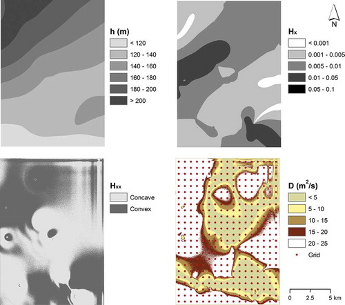
Fig. 7 Plot of hydraulic diffusivities as a function of concomitant storage coefficients, for unconfined, semi-confined and confined aquifers. The literature data were compiled by Pacheco (2013) and Onder (1994). The Szigetvár loess aquifer, with a median diffusivity of D = 17.9 m²/s, behaves as a confined aquifer. The associated storage coefficient is S = bμβS_y = 7.9 × 10^-6, with b = 27.5 m (average aquifer thickness, reported in the ‘Geology’ section), ρ = 999.1 kg/m³ (specific weight of water), β = 4.7 × 10^-9 m²/kg (compressibility of water), and S_y = 0.061 (specific yield, estimated from values in Table 4, based on a median grain size d₅₀ = 0.0405 mm, deduced from data in Table 1).

Fig. 8 Hydraulic head wave (A + B) of a hypothetical heterogeneous aquifer composed of two media, one with a low (A) and the other with a high (B) hydraulic diffusivity.

General relationship between hydraulic diffusivity and scale 

As mentioned in the ‘Results’ section, median hydraulic diffusivities calculated by the GRADIENTS model are comparable with values derived from empirical formulas based on grain-size distributions, when the confined condition is assumed for the tested materials. However Fig. 5 shows that microscale diffusivities can be derived from megascale counterparts if the upper power trend line is extended leftwards to the unit cell size (Δx = 1 m). Finally, in the previous section it was shown that scale effects in hydraulic diffusivity evaluations caused by medium heterogeneity are adequately described by a progressive decrease in the curvature and slope of hydraulic head waves as spatial resolution coarsens. In keeping with these settings, one can bridge hydraulic diffusivity from the microscale to the megascale, with microscale values being associated with unit cell size, and megascale values being upscaled by a factor describing medium heterogeneity as a function of the curvature and slope of associated hydraulic head waves. The general relationship will be a power function relating hydraulic diffusivity with spatial resolution. The base term will comprise the aquifer properties derived from grain-size distributions (hydraulic conductivity and specific yield) and major factors regulating diffusivity at the aquifer-scale (confinement condition and curvature of hydraulic head surface), and an exponent term comprising secondary control parameters of D distribution in space, namely the slope of the hydraulic head surface. The proposed power function for the confined condition is:

(10a)

where L is the spatial resolution (scale). The first base term in brackets represents the confined condition, the second term the microscale hydraulic properties and the third term the changes in curvature of hydraulic head waves (τ_L) relative to values defined at unit spatial resolution (τ₁). The exponent term describes the changes in the wave slope (d_L) relative to values defined at unit spatial resolution (d₁). Switching the confining condition to unconfined, the equation becomes:

(10b)

where b is the saturated aquifer thickness.

Hydraulic diffusivities calculated by equation (10a) were compared with values obtained by the GRADIENTS model, the results being illustrated in Fig. 9(a). Despite the small discrepancies, it is clear that D values are comparable. Figure 9(b) confirms that average head curvatures (τ_L) and slopes (d_L) decrease as scale (heterogeneity) increases.

Fig. 9 (a) Comparison of hydraulic diffusivity estimates, as calculated by the GRADIENTS model and equation (10a). The plot of GRADIENTS model diffusivities is based on D values given in Table 5(a) as a function of Δx (L in the figure). The plot of equation (10a) diffusivities is based on the curvatures and slopes depicted in Table 5(a) as a function of Δx (L in the figure), assuming that τ₁ = τ₁₀ and d₁ = d₁₀. The values of ρ (specific weight of water) and β (compressibility of water) are those referred to in the text. (b) Relationship between the curvature (τ_L) and slope (d_L) of hydraulic head surface (h) and scale (L).

CONCLUSIONS

Hydraulic diffusivity (D) was successfully bridged between the aquifer and the particle-size scales, in the Szigetvár loess area in southwest Hungary. The aquifer or megascale diffusivities were assessed by a finite difference solution of a groundwater flow equation, resulting in a median value D = 17.9 m²/s, typical of a confined aquifer. The particle-size or microscale diffusivities were estimated by empirical laws relating D with statistical parameters of grain-size distributions, resulting in a median value D = 14 m²/s when a confined condition was assumed for the tested materials. In a scatter plot D vs spatial resolution (L), points fitted to a couple of parallel power functions. In the sequel, hydraulic diffusivities were described as a function of microscale diffusivities, interpreted as unit-scale diffusivities, multiplied by a power term where spatial resolution is combined with the concomitant curvature and slope of the hydraulic head surface. Overall, the results obtained in this study demonstrate the compatibility of hydraulic diffusivity estimates based on very different methods and support volumes, providing that an adequate set of methods are selected and a reliable conceptual model is adopted as regards hydraulic head fluctuations, with medium heterogeneity being considered at concomitant scales.

REFERENCES

- Abrisqueta, J.M., et al., 2006. Unsaturated hydraulic conductivity of disturbed and undisturbed loam soil. Spanish Journal of Agricultural Research, 4 (1), 91–96. doi:10.5424/sjar/2006041-179.
- Alyamani, M.S. and Sen, Z., 1993. Determination of hydraulic conductivity from complete grain-size distribution curves. Ground Water, 31, 551–555. doi:10.1111/j.1745-6584.1993.tb00587.x.
- Appoloni, C.R., et al., 1990. Determinação da condutividade e difusividade hidráulica dos solos terra roxa estruturada e latossolo roxo através da infiltração vertical [Determination of hydraulic conductivity and diffusivity of structured red earth and red leptosol through vertical infiltration]. Semina, 11 (4), 145–149.
- Baloochestani, F., 2008. Estimation of hydraulic properties of the shallow aquifer system for selected basins in the Blue Ridge and the Piedmont physiographic provinces of the southeastern U.S. using streamflow recession and baseflow data [online]. Geosciences Dissertations, Paper 2. Available from: http://digitalarchive.gsu.edu/geosciences_diss/2 [Accessed 13 October 2012].
- Bear, J., 1972. Dynamics of fluids in porous media. New York: American Elsevier.
- Beyer, W., 1964. Zur Bestimmung der Wasserdurchlässigkeit von Kiesen und Sanden aus der Kornverteilungskurve. WWT- Wasserwirtschaft Wassertechnik, 14, 165–168.
- Bird, N. and Perrier, E., 2010. Multiscale percolation properties of a fractal pore network. Geoderma, 160, 105–110. doi:10.1016/j.geoderma.2009.10.009.
- Bouma, J., 1982. Measuring the hydraulic conductivity of soil horizons with continuous macropores. Soil Science Society of America Journal, 46, 438–441. doi:10.2136/sssaj1982.03615995004600020047x.
- Butler, J.J., 2005. Hydrogeological methods. In: Y. Rubin and S. Hubbard, eds. Hydrogeophysics. Dordrecht: Springer, 23–58.
- Carman, P.C., 1937. Fluid flow through granular beds. Transactions of the Institution of Chemical Engineers, 15, 150–166.
- Carman, P.C., 1956. Flow of gases through porous media. London: Butterworth Scientific.
- Chen, S.-C., 1998. Estimating the hydraulic conductivity and diffusivity in unsaturated porous media by fractal capillary model. Journal of the Chinese Institute of Engineers, 21 (4), 449–458. doi:10.1080/02533839.1998.9670407.
- Clauser, C., 1992. Permeability of crystalline rocks. Eos, Transactions American Geophysical Union, 73 (21), 233–238. doi:10.1029/91EO00190.
- Das, B.B. and Kondraivendhan, B., 2012. Implication of pore size distribution parameters on compressive strength, permeability and hydraulic diffusivity of concrete. Construction and Building Materials, 28, 382–386. doi:10.1016/j.conbuildmat.2011.08.055.
- De Marsily, G., 1986. Quantitative hydrogeology: groundwater hydrology for engineers. New York: Academic Press.
- Delépine, N., et al., 2004. Characterization of fluid transport properties of the Hot Dry Rock reservoir Soultz-2000 using induced microseismicity. Journal of Geophysics and Engineering, 1, 77–83. doi:10.1088/1742-2132/1/1/010.
- Doan, M.L., et al., 2006. In situ measurement of the hydraulic diffusivity of the active Chelungpu Fault, Taiwan. Geophysical Research Letters, 33, L16317. doi:10.1029/2006GL026889.
- ESRI, 2010. ArcMap (version 10). Redlands, CA: ESRI. Available from: http://www.esri.com/software/arcgis
- Fallico, C., 2014. Reconsideration at field scale of the relationship between hydraulic conductivity and porosity: the case of a sandy aquifer in South Italy. The Scientific World Journal, 2014, 15. doi:10.1155/2014/537387.
- Fischer, U.H., et al., 2001. Hydraulic and mechanical properties of glacial sediments beneath Unteraargletscher, Switzerland: implications for glacier basal motion. Hydrological Processes, 15, 3525–3540. doi:10.1002/hyp.349.
- Flach, G.P., et al., 2000. Electromagnetic Borehole Flowmeter (EBF) testing at the Southwest Plume Test Pad (U). Savannah River Site, Aiken: Westinghouse Savannah River Company (Rep. WSRC-TR–2000–00347).
- Frechen, M., Horváth, E., and Gábris, G., 1997. Geochronology of middle and upper Pleistocene loess sections in Hungary. Quaternary Research, 48, 291–312. doi:10.1006/qres.1997.1929.
- Gilmore, T.J., et al., 1992. Application of three aquifer test methods for estimating hydraulic properties within the 100-N area. Richland, Washington: Pacific Northwest Laboratory (Report US Department of Energy, Contract DE-AC06-76RLO 1830).
- Giménez, D., Rawls, W.J., and Lauren, J.G., 1999. Scaling Properties of saturated hydraulic conductivity in soil. Geoderma, 88, 205–220. doi:10.1016/S0016-7061(98)00105-0.
- Guo, H., Jiao, J.J., and Li, H., 2010. Groundwater response to tidal fluctuation in a two-zone aquifer. Journal of Hydrology, 381, 364–371. doi:10.1016/j.jhydrol.2009.12.009.
- Ha, K., et al., 2007. Estimation of layered aquifer diffusivity and river resistance using flood wave response model. Journal of Hydrology, 337 (3–4), 284–293. doi:10.1016/j.jhydrol.2007.01.040.
- Hazen, A., 1893. Some physical properties of sand and gravels, with special reference to their use in filtration. Twenty Fourth Annual Report of the State Board of Health of Massachusetts, 541–556.
- Heath, R.C., 1983. Basic ground-water hydrology. US Geological Survey Water-Supply Paper 2220.
- Illman, W.A., 2005. Type curve analyses of pneumatic single-hole tests in unsaturated fractured tuff: direct evidence for a porosity scale effect. Water Resources Research, 41, W04018. doi:10.1029/2004WR003703.
- Illman, W.A., 2006. Strong field evidence of directional permeability scale effect in fractured rock. Journal of Hydrology, 319 (1–4), 227–236. doi:10.1016/j.jhydrol.2005.06.032.
- Jámbor, Á.,1997. AKözép-Dunántúlfiatal kainozoos rétegtanának és fejl}odéstörténetének néhány kérdése. Annual Report of the Geological Institute of Hungary 1996 (2), 191–202.
- Jiménez-Martínez, J., et al., 2013. Temporal and spatial scaling of hydraulic response to recharge in fractured aquifers: insights from a frequency domain analysis. Water Resources Research, 49, 3007–3023. doi:10.1002/wrcr.20260.
- Kaubisch, M. and Fischer, M., 1985. Zur Berechnung des Filtrationskoeffizienten in Tagebaukippen. Teil 3: Ermittlung des Filtrationskoeffizienten für schluffige Feinsande aus Mischbodenkippen durch Korngrößenanalysen. Neue Bergbautechnik, 15, 142–143.
- Knudby, C. and Carrera, J., 2006. On the use of apparent hydraulic diffusivity as an indicator of connectivity. Journal of Hydrology, 329, 377–389. doi:10.1016/j.jhydrol.2006.02.026.
- Kovács, J., et al., 2011. Plio-Pleistocene red clay deposits in the Pannonian basin: a review. Quaternary International, 240 (1–2), 35–43. doi:10.1016/j.quaint.2010.12.013.
- Krahn, J., 2004. Transport modelling with CTRAN/W: an engineering methodology. Calgary: GEO-SLOPT International.
- Leahy, P.P., 1976. Hydraulic characteristics of the Piney Point aquifer and overlying confining bed near Dover. Dover, DE: Geological Survey, Report of investigations 26.
- Le Borgne, T., et al., 2006. Assessment of preferential flow path connectivity and hydraulic properties at single borehole and cross-borehole scales in a fractured aquifer. Journal of Hydrology, 328, 347–359. doi:10.1016/j.jhydrol.2005.12.029.
- Li, V.C., 1984. Estimation of in-situ hydraulic diffusivity of rock masses. Pure and Applied Geophysics, 122, 545–559. doi:10.1007/BF00874616.
- Martinez-Landa, L. and Carrera, J., 2005. An analysis of hydraulic conductivity scale effects in granite (Full-scale Engineered Barrier Experiment (FEBEX), Grimsel, Switzerland. Water Resources Research, 41, W03006.
- Morris, D.A. and Johnson, A.I., 1967. Summary of hydrologic and physical properties of rock and soil materials, as analyzed by the hydrologic laboratory of the U.S. Geological Survey (1948–60). US Geological Survey Water-Supply Paper 1839-D.
- Murray, T., 1997. Assessing the paradigm shift: deformable glacier beds. Quaternary Science Reviews, 16, 995–1016. doi:10.1016/S0277-3791(97)00030-9.
- Nemecz, E., et al., 2000. The origin of the silt size quartz grains and minerals in loess. Quaternary International, 68–71, 199–208. doi:10.1016/S1040-6182(00)00044-6.
- Neuman, S.P., 1990. Universal scaling of hydraulic conductivities and dispersivities in geologic media. Water Resources Research, 26, 1749–1758. doi:10.1029/WR026i008p01749.
- Neuman, S.P. and Witherspoon, P.A., 1972. Field determination of the hydraulic properties of leaky multiple aquifer systems. Water Resources Research, 8 (5), 1284–1298. doi:10.1029/WR008i005p01284.
- Odong, J., 2007. Evaluation of empirical formulae for determination of hydraulic conductivity based on grain-size analysis. Journal of American Science, 3 (3), 54–60.
- Onder, H., 1994. Determination of aquifer parameters of finite confined aquifers from constant drawdown nonsteady type-curves. Hydrological Sciences Journal, 39 (3), 269–280. doi:10.1080/02626669409492743.
- Pacheco, F.A.L., 2013. Hydraulic diffusivity and macrodispersivity calculations embedded in a geographic information system. Hydrological Sciences Journal, 58 (4), 930–944. doi:10.1080/02626667.2013.784847.
- Pacheco, F.A.L. and Alencoão, A.M.P., 2006. Role of fractures in weathering of solid rocks: narrowing the gap between laboratory and field weathering rates. Journal of Hydrology, 316 (1–4), 248–265. doi:10.1016/j.jhydrol.2005.05.003.
- Pacheco, F.A.L. and Szocs, T., 2006. Dedolomitization reactions” driven by anthropogenic activity on loessy sediments, SW Hungary. Applied Geochemistry, 21, 614–631. doi:10.1016/j.apgeochem.2005.12.009.
- Pacheco, F.A.L. and Van der Weijden, C.H., 2012. Weathering of plagioclase across variable flow and solute transport regimes. Journal of Hydrology, 420–421, 46–58. doi:10.1016/j.jhydrol.2011.11.044.
- Pécsi, M., 1987. The loess-paleosol and related subaereal sequence in Hungary. Geojournal, 15 (2), 151–162.
- Pradhana, B., Nageshb, M., and Bhattacharjee, B., 2005. Prediction of the hydraulic diffusivity from pore size distribution of concrete. Cement and Concrete Research, 35, 1724–1733. doi:10.1016/j.cemconres.2004.10.043.
- Rovey, C.W. and Cherkauer, D.S., 1995. Scale dependency of hydraulic conductivity measurements. Ground Water, 33, 769–780. doi:10.1111/j.1745-6584.1995.tb00023.x.
- Schad, H. and Teutsch, G., 1994. Effects of the investigation scale on pumping test results in heterogeneous porous aquifers. Journal of Hydrology, 159, 61–77. doi:10.1016/0022-1694(94)90249-6.
- Schulze-Makuch, D. and Cherkauer, D.S., 1997. Method developed for extrapolating scale behavior. Eos, Transactions American Geophysical Union, 78, 3. doi:10.1029/97EO00005.
- Schulze-Makuch, D. and Cherkauer, D.S., 1998. Variations in hydraulic conductivity with scale of measurement during aquifer tests in heterogeneous, porous, carbonate rocks. Hydrogeology Journal, 6, 204–215. doi:10.1007/s100400050145.
- Schulze-Makuch, D., et al., 1999. Scale dependency of hydraulic conductivity in heterogeneous media. Ground Water, 37, 904–919. doi:10.1111/j.1745-6584.1999.tb01190.x.
- Seelheim, F., 1880. Methoden zur Bestimmung der Durchlässigkeit des Bodens. Fresen. Zeitschrift für Analytische Chemie, 19, 387–418. doi:10.1007/BF01341054.
- Shepherd, R.G., 1989. Correlations of permeability and grain sizes. Ground Water, 27, 633–638. doi:10.1111/j.1745-6584.1989.tb00476.x.
- Shih, D. and Lin, G., 2004. Application of spectral analysis to determine hydraulic diffusivity of a sandy aquifer(Pingtung County, Taiwan). Hydrological Processes, 18 (9), 1655–1669. doi:10.1002/hyp.1411.
- Smalley, I.J. and Leach, J.A., 1978. The origin and distribution of the loess in the Danube basin and associated regions of East-Central Europe—A review. Sedimentary Geology, 21, 1–26. doi:10.1016/0037-0738(78)90031-3.
- Talwani, P., 1976. Earthquakes associated with the Clark Hill reservoir, South Carolina—A case of induced seismicity. Engineering Geology, 10, 239–253. doi:10.1016/0013-7952(76)90024-7.
- Talwani, P., 1997. On the nature of reservoir-induced seismicity. Pure Applied Geophysics, 150, 473–492. doi:10.1007/s000240050089.
- Talwani, P., Cobb, J.S., and Schaeffer, M.F., 1999. In situ measurements of hydraulic properties of a shear zone in northwestern South Carolina. Journal of Geophysical Research, 104 (B7), 14993–15003. doi:10.1029/1999JB900059.
- Taylor, C.J. and Alley, W.M., 2001. Ground-water-level monitoring and the importance of long-term water-level data. Denver, CO: US Geological Survey Circular 1217.
- Terzaghi, K. and Peck, R.B., 1964. Soil mechanics in engineering practice. New York: Wiley.
- Trefry, M.G. and Johnston, C.D., 1998. Pumping test analysis for a tidally forced aquifer. Ground Water, 36 (3), 427–433. doi:10.1111/j.1745-6584.1998.tb02813.x.
- Van der Kamp, G., 2001. Methods for determining the in situ hydraulic conductivity of shallow aquitards – an overview. Hydrogeology Journal, 9 (1), 5–16. doi:10.1007/s100400000118.
- Vesselinov, V.V., Neuman, S.P., and Illman, W.A., 2001. Threedimensional numerical inversion of pneumatic cross-hole tests in unsaturated fractured tuff: 2. Equivalent parameters, high-resolution stochastic imaging and scale effects. Water Resources Research, 37, 3019–3041. doi:10.1029/2000WR000135.
- Vienken, T. and Dietrich, P., 2011. Field evaluation of methods for determining hydraulic conductivity from grain size data. Journal of Hydrology, 400, 58–71. doi:10.1016/j.jhydrol.2011.01.022.
- Vuković, M. and Soro, A., 1992. Determination of hydraulic conductivity of porous media from grain-size composition. Littleton, CO: Water Resources Publications.
- Wibberley, C.A.J., 2002. Hydraulic diffusivity of fault gouge zones and implications for thermal pressurization during seismic slip. Earth Planets Space, 54, 1153–1171.