An automated inverse method for slug tests—over-damped case—in confined aquifers

Abstract

Slug tests offer an efficient method for estimating the hydraulic parameters of an aquifer without water pumping. Two inverse methods are typically used to assess the slug test data and derive parameter estimates of a confined aquifer. The first method provides estimates of both hydraulic conductivity and specific storage, is visual (hence difficult to automate), and is based on the transient-flow analytical solution of Cooper et al. The second method, proposed by Hvorslev, is very straightforward, but provides only hydraulic conductivity estimates. In this study, we are testing the recently proposed quasi-steady method of Koussis and Akylas, which enables the estimation of both hydraulic parameters and, furthermore, can be easily implemented in computer code or an electronic spreadsheet. This quasi-steady method was coupled with the shuffled complex evolution optimization method to fully automate parameter estimation. This coupling is tested using data from field observations, synthetic data produced from the transient-flow analytical solution, and synthetic data with noise. The results show the usefulness and the limitations of the proposed method.

Editor Z.W. Kundzewicz

Résumé

Les essais d’injection sont une méthode efficace pour estimer les paramètres hydrauliques d’un aquifère sans pompage d’eau. Deux méthodes inverses sont généralement utilisées pour évaluer les données des essais d’injection et obtenir des estimations des paramètres d’un aquifère captif. La première méthode, qui fournit des estimations de la conductivité hydraulique et de l’emmagasinement spécifique, est visuelle (donc difficile à automatiser) et est basée sur la solution analytique du régime transitoire de Cooper et al. La seconde méthode, proposée par Hvorslev, est très simple mais ne fournit que des estimations de la conductivité hydraulique. Dans cette étude, nous testons la méthode du régime quasi-permanent récemment proposée par Koussis et Akylas qui permet d’estimer les deux paramètres hydrauliques et peut être facilement mise en œuvre dans un code informatique ou une feuille de calcul. Cette méthode de quasi-équilibre a été couplée avec la méthode d’optimisation « Shuffled Complex Evolution » pour automatiser entièrement l’estimation des paramètres. Ce couplage a été testé en utilisant de données de terrain, de données synthétiques produites à partir de la solution analytique en régime transitoire et de données synthétiques bruitées. Les résultats montrent l’utilité et les limitations de la méthode proposée.

Key words:

• confined aquifers
• optimization
• parameters estimation
• SCE method
• slug test

Mots clefs:

• aquifères captifs
• optimisation
• estimation des paramètres
• méthode SCE
• essai d’injection

1 INTRODUCTION

Slug tests offer an efficient means of estimating the hydraulic parameters of a geological formation and are very well suited to contaminated site assessment, because no water is withdrawn. In this in situ test, head variations are generated in the aquifer through an initial rapid change of water level in the borehole, H_o, from static conditions induced by either adding or bailing water, by placing a metal piece (a slug) in the well casing causing a change in the water level or pneumatically. The hydraulic parameters of a confined aquifer, the radial hydraulic conductivity K_r and the coefficient of specific storage S_s, are determined by an inverse procedure in which the monitored variation of the head inside the borehole, H(t), is compared to head responses—type curves—computed by a theoretical model for a series of assumed values of these parameters.

The established procedure is based on the transient-flow analytical solution of Cooper et al. (1967) of a slug test for over-damped conditions carried out in a well fully penetrating a confined aquifer:

(1)

where J_i and Y_i are Bessel functions of ith order of the first and second kinds, respectively; β = K_rbt/r_c² is dimensionless time; α = r_s²S_sb/r_c² is a dimensionless storage parameter; b is the formation thickness; r_s is the effective radius of the well screen; and r_c is the effective radius of the well casing.

However, this procedure is computationally involved and awkward to use. Thus, groundwater professionals often use a few pre-prepared type curves H(t)/H_o = f(β,α) to fit the normalized head response data by a visual matching procedure and to calculate the hydraulic parameters of the formation. The matching procedure of Cooper et al. (1967) is as follows: (a) fit the observations optimally with a type curve (α_opt) (abscissas must have scales with equal number of log-cycles); (b) select a convenient match point, e.g. β = 1, for which the time t_β=1.0 is read off the x-axis of the data plot ; and (c) use the definitions of α and β, with β = 1, t_β=1.0 and α_opt, to compute K_r = r_c²/bt_β-1.0 and S_s = α_optr_c²/r_s²b.

In contrast, the very straightforward method of Hvorslev (1951) focuses only on the head variation inside the well to yield an estimate of the conductivity of a formation, but it cannot estimate the specific storage coefficient, because it ignores the storage balance inside the aquifer. Koussis and Akylas (2012) have developed an inverse procedure that considers the flow in the aquifer to be quasi-steady; this method is much simpler than Cooper’s method (compare equation (1) with equations (2) and (3)), yet it provides estimates for K_r and for S_s. In a quasi-steady solution, a series of steady states substitutes the transient process, considering the physical system to evolve in abrupt steps from one steady state to the next one. This is a well-established concept in subsurface hydrology, dating back to Lembke (1887) and still in use (e.g. Verhoest and Troch (2000), Akylas et al. (2006) and Rozos and Koutsoyiannis (2010)). Besides subsurface hydrology, Adams and Koussis (1980) have also analysed the response of cooling ponds to transient atmospheric forcing with the quasi-steady approach.

The operational equations of this quasi-steady flow model are as follows:

(2)

(3)

in which R(t) is the unknown time-varying radial distance to the edge of the quasi-steady flow domain (radius of influence), where the head lowering/rising in the aquifer vanishes, i.e. H(R) = 0. These two equations form a system of nonlinear equations that is solved numerically (see Appendix).

This model closely approximates the model of Cooper et al. (1967) and has the practical advantage that its solution type curves can be generated very simply, e.g. with an electronic spreadsheet, for use in matching the (dimensionless) well response data (Koussis and Akylas 2012). Therefore, an optimal fit of observation data by a solution curve could be readily embedded in a manual exhaustive search. That search procedure, however, would be heuristic, involving repeated computation of the quasi-steady flow solution, until locating an optimal pair of K_r and S_s values, visually or according to some criterion of optimality. In the sequel, we present a fully automated inverse procedure for estimating the optimal hydraulic formation parameters K_r and S_s that uses the quasi-steady flow solution and a formal optimization method. Then, we test this inverse procedure on three field slug tests and on a series of synthetic data that correspond to hypothetical confined aquifers with a wide range of hydraulic properties.

2 OPTIMIZATION

In order to automate the estimation of both hydraulic formation parameters, K_r and S_s, we coupled the quasi-steady (QS) flow solution with the shuffled complex evolution (SCE) optimization method (Duan et al. 1992). The SCE method is based on a synthesis of four concepts that have been proven successful for global optimization: (a) combination of probabilistic and deterministic approaches; (b) clustering; (c) systematic evolution of a complex of points spanning the space in the direction of global improvement; and (d) competitive evolution (Duan et al. 1993). The algorithm starts by sorting into groups, or complexes, an initial population of points in the n-dimensional parameter space. Then, the algorithm evolves the population of each complex using a geometric-probabilistic approach. Afterwards, the complexes are shuffled, to share the information gained by each complex independently, and the algorithm starts over again, until convergence is achieved.

The objective function used in the optimization is the root mean square error between the normalized measurements of head, H/H_o, and the HH0_j values calculated by the QS solution. The objective function exhibits multiple minima at all scales and hence cannot be minimized with a more straightforward algorithm (e.g. Fibonacci search algorithm). Instead, a global optimization algorithm, like the SCE method here, must be employed.

Because the dimensionless time steps β_j of HH0_j values and the dimensionless time steps of the measurements are not expected to coincide, linear interpolation is used. The logarithms of K_r and S_s are used as arguments of the objective function (which wraps the QS method) instead of the plain values, to tackle the wide range of parameter values that extend over several orders of magnitude (Efstratiadis et al. 2008). The optimization uses only the measurements with H/H_o > 1/3. This is dictated by the lesser accuracy of the QS solution for small H/H_o values (see Fig. 2 of Koussis and Akylas 2012), probably because of imposing the condition H = 0 at r = R instead of at r → ∞. An apparent side effect of this restriction is that since the S-curves (see right panel of Fig. 1) are differentiated between each other mainly by the shape of their two bends and since the lower bend is omitted due to the H/H_o > 1/3 restriction, a sufficient number of measurements should exist on the upper bend of the S-curve.

Fig. 1 Measurements actually used in Hvorslev’s method as recommended by Butler (left panel) and in the QS method (right panel).

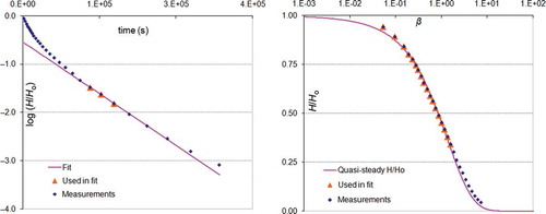
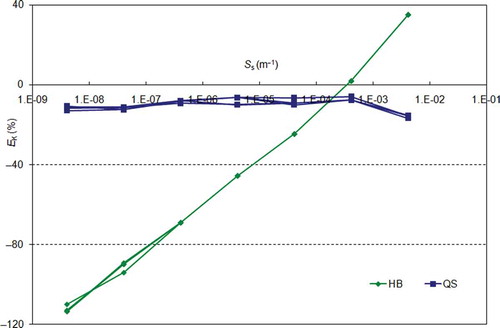
Fig. 2 Dependence of K_r estimation error (E_K) on S_s; E_K = 10.43 ln(S_s ×1 m) + 85.72 fits the HB points with r² = 0.99.

It should be noted that Butler (1998) has also suggested a restriction on the data actually used in the inverse solution with Hvorslev’s method. The condition that Butler introduced to decide whether a measurement should be used, or not, is for H/H_o to lie between 0.15 and 0.25. Figure 1 displays the fit to slug test measurements (taken from Butler (1998)) of the curves created by Hvorslev’s method and the QS method. The measurements actually used in Hvorslev’s method following Butler’s suggestion (left panel) and in the QS method (right panel) are highlighted with orange triangles.

3 IMPLEMENTATION

The algorithm that solves the nonlinear system of equations of the QS method (equations (4)–(6)), the objective function and some support scripts (100 lines of code in total) were implemented in MATLAB m-files (also compatible with GNU Octave). The SCE algorithm code was obtained from MATLAB CENTRAL (Duan 2013). For execution, the automated parameter optimization procedure requires a two-column csv file containing the absolute time (in seconds) and normalized head observations in semicolon-separated data fields, and a text file with the aquifer thickness, screen radius and casing radius. To visualize how the optimal QS type curve fits the measurements, csv files are prepared that can be plotted and analysed with a spreadsheet.

To make this software available without requiring installation of MATLAB or Octave, a stand-alone version was prepared based on the Octave 3.6.2 engine. The model runs as a command-prompt application providing the user with a menu of the available actions, to: (a) run the QS method to determine the optimal set of hydraulic formation parameters, K_r and S_s; (b) prepare a csv file of the type curve optimally fitting the data for exporting to a spreadsheet; (c) run Hvorslev’s method; (d) run Hvorslev’s method as suggested by Butler (see Fig. 1 (left panel)); and (e) quit. A typical optimization run completes in ~4 s on a PC with a 3.4 GHz CPU. This software package is named HydroCthon—chthon is an ancient Greek word for earth; chthonic pertains to underworld deities in Greek mythology.

4 APPLICATION TO FIELD OBSERVATIONS

The reliability of the proposed automated method was tested initially using three time series derived from field measurements. The first one was derived from a slug test at the Lincoln County monitoring site (Table 5.2 of Butler 1998). The aquifer thickness b, the screen radius r_s and the casing radius r_c were 3.05, 0.071 and 0.025 m, respectively (Butler 1998, Table 5.1). According to Butler, the visual matching of the measurements with the type curves of Cooper et al. (1967) yields the estimates K_r = 3.69 × 10^-4 m d^-1 and S_s = 4.38 × 10^-4 m^-1. The second series of measurements was taken from Todd and Mays (2005); the reference values are K_r = 1.006 m d^-1 and S_s = 4.94 × 10^-5 m^-1. The third series is from well DOW-4 in the Deerfield site (Test 4, Figures 16–19 in Butler and Healey 1998), with reference values K_r = 21.9 m d^-1 (72 ft d^-1) and S_s = 4.59 × 10^-8 m^-1 (1.4 × 10^-8 ft^-1). It should be noted that any reference values of real aquifers are estimates derived with a method of good accuracy, not the (unknown) actual values of the hydraulic parameters of the aquifer.

In the case of the Lincoln County slug test, the QS-SCE method estimated the hydraulic parameters as K_r = 3.71 × 10^-4 m d^-1 and S_s = 5.14 × 10^-4 m^-1. Therefore, the estimation errors are E_K = 0.5% and E_S = 17.4%. In the case of the slug test data in Todd and Mays (2005), the QS-SCE method estimated the hydraulic parameters as K_r = 8.94 × 10^-1 m d^-1 and S_s = 1.62 × 10^-4 m^-1. Therefore, the estimation errors are E_K = −11.1% and E_S = 227.9%. Finally, for the Deerfield site, the estimated hydraulic parameters are K_r = 21.7 m d^-1 and S_s = 6.9 × 10^-8 m^-1, with E_K = –0.9% and E_S = 50.3%. Regarding the Deerfield data, Butler and Healey (1998) note that the optimal fit of the Cooper et al. (1967) model was accomplished with an implausibly low S_s value (as is the QS-SCE S_s value), however, they considered the estimated hydraulic conductivity value to be reasonable, and unaffected by low-K skin or vertical flow, which is reassuring for the estimation ability of the QS-SCE method.

For comparison, the K_r estimate of Hvorslev’s method with R/r_s = 200 (recommended by the US Navy (Butler 1998)) and fitting a straight line to only the nearly-linear mid portion of the data (mentioned hereafter as Hvorslev-Butler method, or just HB), was for the first case study 3.88 × 10^-4 m d^-1, for the second 9.01 × 10^-1 m d^-1 and for the third 9.7 m d^-1. The corresponding estimation errors E_K are  5.1%, −10.4% and 55.7%, respectively (see Table 1). The sizeable error of the HB estimate in the Deerfield case must be attributed to non-negligible elastic storage effects indicated by a concave-upward curvature of the semi-logarithmic plot of the response data (Butler 1998, p. 68).

Table 1 Comparison of QS, HB and Hvorslev (Hv) estimations using field observations.

	Lincoln County	Todd-Mays	Deerfield site
Ref.	3.69 × 10^-4 m d^-1 | 4.38 × 10^-4 m^-1	1.01 × 10 ^0 m d^-1 | 4.94 × 10^-5 m^-1	21.9 × 10^0 m d^-1 | 4.59 × 10^-8 m^-1
QS	3.71 × 10^-4 m d^-1 | 5.14 × 10^-4 m^-1	8.94 × 10^-1 m d^-1 | 1.62 × 10^-4 m^-1	21.7 × 10^0 m d^-1 | 6.85 × 10^-8 m^-1
HB	3.88 × 10^-4 m d^-1 |	9.01 × 10^-1 m d^-1 |	9.71 × 10^0 m d^-1 |
Hv.	4.65 × 10^-4 m d^-1 |	8.30 × 10^-1 m d^-1 |	9.71 × 10^0 m d^-1 |

Table 1 also compares the HB method against the original Hvorslev’s method (fit a straight line to all measurements). In two of the three cases, the original method had worse performance whereas in the third case the original method and the HB were equivalent. This verifies the credibility of the HB method, which should be preferred over the original one.

5 APPLICATION TO SYNTHETIC DATA

To further test our method under a wide range of K_r and S_s values, we used synthetic data. As a first step to produce these ‘observations’, K_r and S_s reference values were chosen. The chosen reference values were 2.02 × 10^-4, 2.02 × 10^-2, 1, 10 and 100 m d^-1 for K_r and 4.07 × 10^-3, 4.07 × 10^-4, 4.07 × 10^-5, 4.07 × 10^-6, 4.07 × 10^-7, 4.07 × 10^-8 and 4.07 × 10^-9 m^-1 for S_s. Therefore, five K_r reference values combined with seven S_s reference values give 35 (K_r, S_s) pairs. From these 35 pairs and assuming identical values of b, r_s and r_c to those of the Lincoln site slug test, 35 measurement time series were produced with the following procedure:

• The dimensionless storage parameter α = r_s²S_sb/r_c² was calculated for each (K_r, S_s) pair.

• several pairs of normalized head values H/H_o vs dimensionless times β_i were obtained from the Cooper pre-prepared type curves for each α (Table 5.14.1a of Todd and Mays 2005).

• The absolute time t_i corresponding to each normalized head value H/H_o was calculated with the formula t_i = β_ir_c²/K_rb.

The results of the optimizations are summarized in Tables 2–4 (note: values of Tables 2 and 3 should be compared against the column heading, whereas values of Table 4 should be compared against the row heading). According to these results, the estimation error of K_r for the QS and HB methods was not influenced by the magnitude of K_r (nor was the estimation error of S_s in the QS method). However, the obtained results indicate that the estimation error was influenced by the magnitude of S_s, especially in the HB method.

Table 2 Estimated K_r values (note: compare against column heading) with QS method using synthetic observations.

	2.02 × 10^-4 (m d^-1)	2.02 × 10^-2 (m d^-1)	1.00 (m d^-1)	10 (m d^-1)	100 (m d^-1)
4.07 × 10^-3 m^-1	1.75 × 10^-4	1.75 × 10^-2	8.56 × 10^-1	8.66	86.57
4.07 × 10^-4 m^-1	1.88 × 10^-4	1.87 × 10^-2	9.28 × 10^-1	9.28	94.31
4.07 × 10^-5 m^-1	1.85 × 10^-4	1.83 × 10^-2	9.16 × 10^-1	9.15	93.85
4.07 × 10^-6 m^-1	1.83 × 10^-4	1.89 × 10^-2	9.09 × 10^-1	9.40	93.94
4.07 × 10^-7 m^-1	1.87 × 10^-4	1.87 × 10^-2	9.14 × 10^-1	9.26	92.41
4.07 × 10^-8 m^-1	1.79 × 10^-4	1.79 × 10^-2	8.96 × 10^-1	8.99	88.91
4.07 × 10^-9 m^-1	1.82 × 10^-4	1.78 × 10^-2	8.96 × 10^-1	8.98	90.30

Table 3 Estimated K_r values (note: compare against column heading) with HB method using synthetic observations.

	2.02 × 10^-4(m d^-1)	2.02 × 10^-2 (m d^-1)	1.00 (m d^-1)	10 (m d^-1)	100 (m d^-1)
4.07 × 10^-3 m^-1	2.73 × 10^-4	2.73 × 10^-2	1.35 × 10 ^0	13.50	135.00
4.07 × 10^-4 m^-1	2.06 × 10^-4	2.06 × 10^-2	1.02 × 10 ^0	10.20	102.00
4.07 × 10^-5 m^-1	1.62 × 10^-4	1.62 × 10^-2	8.02 × 10^-1	8.13	80.20
4.07 × 10^-6 m^-1	1.39 × 10^-4	1.39 × 10^-2	6.87 × 10^-1	6.87	68.70
4.07 × 10^-7 m^-1	1.19 × 10^-4	1.19 × 10^-2	5.91 × 10^-1	5.91	59.10
4.07 × 10^-8 m^-1	1.07 × 10^-4	1.06 × 10^-2	5.15 × 10^-1	5.27	52.67
4.07 × 10^-9 m^-1	9.46 × 10^-5	9.49 × 10^-3	4.76 × 10^-1	4.68	46.84

Table 4 Estimated S_s values (note: compare against row heading) with QS method using synthetic observations.

	2.02 × 10^-4 (m d^-1)	2.02 × 10^-2 (m d^-1)	1.00 (m d^-1)	10 (m d^-1)	100 (m d^-1)
4.07 × 10^-3 m^-1	6.27 × 10^-3	6.30 × 10^-3	6.41 × 10^-3	6.28 × 10^-3	6.28 × 10^-3
4.07 × 10^-4 m^-1	6.65 × 10^-4	6.65 × 10^-4	6.66 × 10^-4	6.65 × 10^-4	6.31 × 10^-4
4.07 × 10^-5 m^-1	8.84 × 10^-5	9.14 × 10^-5	8.84 × 10^-5	8.87 × 10^-5	7.69 × 10^-5
4.07 × 10^-6 m^-1	1.17 × 10^-5	9.54 × 10^-6	1.16 × 10^-5	9.48 × 10^-6	9.51 × 10^-6
4.07 × 10^-7 m^-1	1.27 × 10^-6	1.28 × 10^-6	1.45 × 10^-6	1.28 × 10^-6	1.31 × 10^-6
4.07 × 10^-8 m^-1	2.51 × 10^-7	2.47 × 10^-7	2.27 × 10^-7	2.17 × 10^-7	2.51 × 10^-7
4.07 × 10^-9 m^-1	2.72 × 10^-8	3.55 × 10^-8	2.93 × 10^-8	2.91 × 10^-8	2.70 × 10^-8

Figure 2 shows how the estimation error of K_r varies with S_s for the QS and HB methods. In this figure, the results of each method are represented with a different group of lines (i.e. two groups for the two methods), with each individual line of each group corresponding to a different K_r value (lines of each group almost coinciding, which indicates that the estimation error of K_r does not depend on the magnitude of K_r).

Figure 2 indicates that the S_s magnitude does not have significant impact on the K_r estimation error of the QS method. On the contrary, the K_r estimation error of the HB is influenced significantly. This behaviour has been detected also by Butler (1998), who notes that a distinct concave-upwards curvature in the semi-log plot of measurements indicates that the influence of elastic storage cannot be neglected and therefore the accuracy of Hvorslev’s method is reduced.

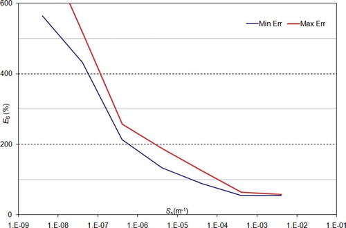
Figure 3 presents the dependence of the S_s estimation error on the magnitude of S_s (the two lines give the maximum and minimum estimation errors of the five reference K_r). According to this figure, the estimation error (computed by the formula (Est. − Ref.)/min(Est., Ref.)) depends strongly on the magnitude of S_s, with the error rising sharply for S_s values smaller than ~5 × 10^-8. This is attributed to the fact that the QS solution curves, like those of Cooper et al. (1967), become almost parallel for small S_s values. However, it should be noted that, for S_s values greater than ~5 × 10^-6 m^-1, the QS method estimates correctly the order of magnitude of S_s.

Fig. 3 Dependence of S_s estimation error (E_S) on S_s.

6 APPLICATION TO SYNTHETIC DATA WITH NOISE

As a final test, and in order to check the influence of measurement error on the efficiency of the automated method, we combined six sets of time series of white noise ξ (1000 series in each set with length equal to the length of measurements) with the six synthetic measurements corresponding to the reference values that can been seen in Tables 5 and 6 (reference S_s in first row and reference K_r in caption of these tables). The noise ξ follows the normal distribution (0 m, 0.025 m) normalized by H_o, which was assumed equal to 2 m. The standard deviation 0.025 m corresponds to the worst precision that Sorensen and Butcher (2011) mention, after comparing 19 transducers from 14 leading brands (i.e. the standard deviation 0.025 m corresponds to the less accurate instrument of that study). The series of measurements with noise were produced using the formula , where the H/H_o values were taken from the Cooper et al. (1967) type curves, as explained above.

Table 5 Normalized statistical metrics of QS and HB methods for K_r = 2.02 × 10^-4 m d^-1 derived using synthetic observations with errors.

Ref Ss (m^-1)	4.07 × 10^-5	4.07 × 10^-4	4.07 × 10^-3
QS Kr RMSE (%)	18.3	18.0	27.5
QS Ss RMSE (%)	355.6	149.7	118.6
HB Kr RMSE (%)	30.8	18.6	30.8

The performance of the QS and HB was evaluated using as a statistical metric, the relative (i.e. normalized by the reference value) root mean square error. The latter is calculated as the RMSE between the 800 estimated values and corresponding reference values (K_r and S_s are estimated for each one of the 1000 synthetic measurements with noise of each one of the six sets, but only the 800 that fall in the 10–90% quantile are used in the calculation of the RMSE to exclude the synthetic measurements with unrealistic errors).

Tables 5 and 6 provide the statistical metrics for K_r and S_s estimated by QS and for K_r estimated by HB. The corresponding values of these two tables differ slightly, verifying the previous findings that the magnitude of K_r does not influence significantly the estimation reliability of either method. The RMSE of the HB method seems to have a linear relationship with S_s. The RMSE of the QS method seems constant for S_s ≤ 4.07 × 10^-4 m^-1. For these values of S_s, the RMSE of the QS method is considerably lower than that of HB, implying better estimations of K_r. For larger S_s values, the RMSE of the QS method is just slightly lower. Finally, the RMSE of S_s estimates increases considerably for S_s < 4.07 × 10^-4 m^-1. This finding is in agreement with Papadopulos et al. (1973), who noted that the reliability of the S_s estimation becomes questionable for α < 10^-5, since “Even the most carefully and accurately collected test data could easily be matched with more than one of the type curves. The best one could expect, is to be within one or two orders of magnitude of the actual value”. It should be mentioned that the difficulty of estimating S_s is generally admitted (see Butler 1998) and has been already pointed out by Cooper et al. (1967). McElwee et al. (1995) noted that single-well slug tests do not provide good estimates of specific storage due to the insensitivity of test responses to the storage parameter and uncertainty regarding the effective screen radius.

Table 6 Normalized statistical metrics of QS and HB methods for K_r = 1 m d^-1 derived using synthetic observations with errors.

Ref Ss (m^-1)	4.07 × 10^-5	4.07 × 10^-4	4.07 × 10^-3
QS Kr RMSE (%)	17.7	17.1	26.9
QS Ss RMSE (%)	329.9	144.1	114.9
HB Kr RMSE (%)	29.8	18.1	31.9

7 SUMMARY AND CONCLUSIONS

In this study we have presented an automated inverse method for estimating the hydraulic parameters K_r and S_s of confined aquifers from slug test measurements for the over-damped case. This method is based on the coupling of the quasi-steady flow solution of Koussis and Akylas (2012) and the shuffled complex evolution (SCE) optimization method of Duan et al. (1992). The developed software package is available as a stand-alone application, based on the Octave 3.6.2 engine (it does not require installation of MATLAB or Octave), and runs efficiently as a command-prompt application, providing the user with a simple menu of the available actions for the optimal estimation of K_r and S_s. It also facilitates visualising how the solution or type curve calculated with the estimated hydraulic parameters fits the data and exporting the results to a spreadsheet for further analysis. To test the coupled quasi-steady solution – SCE optimization method, field and synthetic observations were used, the latter with and without error. The performance of the proposed method was also compared against that of the established method of Hvorslev-Butler for estimating the hydraulic conductivity. The tests indicated that:

• The coupled quasi-steady solution – SCE optimization method performs generally well, providing K_r estimates of high quality. Useful estimates of S_s, i.e. of the correct order of magnitude, can be obtained for S_s values greater than 5 × 10^-6, provided the measurement error is low. If there is significant measurement error, then the magnitude threshold for obtaining useful S_s estimates rises to ~10^-4 m^-1.

• The reliability of the optimal K_r estimates determined by the quasi-steady solution – SCE optimization method is influenced marginally by the magnitude of S_s. In contrast, the reliability of Hvorslev’s K_r estimates appears to depend strongly on S_s. However, the magnitude of K_r does not influence significantly the K_r estimates of either method (and the S_s estimates of the quasi-steady method).

• The quasi-steady solution – SCE optimization method uses measurements that have H/H_o greater than 0.33 and requires measurements with H/H_o greater than 0.8 to be accurate. The Hvorslev-Butler method uses only measurements that have H/H_o values between 0.15 and 0.25.

The parameter estimation software HydroCthon—the quasi-steady flow method of slug test analysis of Koussis and Akylas (2012) combined with the shuffled complex evolution optimization method—along with the data used in this study are available for downloading and testing at: http://itia.ntua.gr/en/softinfo/30/.

APPENDIX

The system of nonlinear equations (2) and (3) can be solved numerically with the following algorithm.

• Set the variable y : = R/r_s and compute it in n non-constant increments, i.e. y_j = y_j-1 + Δy_j with y₀ = 1, Δy_j = 0.015 exp(0.015 j) and j = 0, 1, ..., n (n should be large enough to ensure that β_n, last value of β_j calculated by equation (A3), is greater than the maximum dimensionless time of measurements).

• For each value y_j, calculate a value of F(y_j) by the formula (term in parentheses on the right-hand side of equation (2)):

  (A1)

• Set HH0_j : = H(β_j)/H_o, i.e. the value of H/H_o at the dimensionless time β_j. Then, estimate the pairs (HH0_j, β_j), which give the curves of the quasi-steady (QS) solution, with the following formulae:

  (A2)
  (A3)

REFERENCES

- Adams, E.E. and Koussis, A.D., 1980. Transient analysis for shallow cooling ponds. Journal of Energy Engineering (ASCE), 106 (EY2), 141–153.
- Akylas, E., Koussis, A.D., and Yannacopoulos, A.N., 2006. Analytical solution of transient flow in a sloping soil layer with recharge. Hydrological Sciences Journal, 51 (4), 626–641. doi:10.1623/hysj.51.4.626.
- Butler, J.J., 1998. The design, performance, and analysis of slug tests. Boca Raton, FL: Lewis Publishers.
- Butler, J.J. and Healey, J.M., 1998. Performance and analysis of June 1998 and October 1999 slug tests in Kearny, Finney, and Ford Counties, Kansas. Kansas Geological Survey, Open-file Report 1999-8.
- Cooper, H.H., Bredehoeft, J.D., and Papadopulos, I.S., 1967. Response of a finite-diameter well to an instantaneous charge of water. Water Resources Research, 3 (1), 263–269. doi:10.1029/WR003i001p00263.
- Duan, Q., 2013. Shuffled complex evolution method (SCE-UA). Available from MATLAB CENTRAL: http://www.mathworks.com/matlabcentral/fileexchange/7671 [Accessed January 2013].
- Duan, Q., Gupta, V.K., and Sorooshian, S., 1993. Shuffled complex evolution approach for effective and efficient global minimization. Journal of Optimization Theory and Applications, 76, 501–521. doi:10.1007/BF00939380.
- Duan, Q., Sorooshian, S., and Gupta, V., 1992. Effective and efficient global optimization for conceptual rainfall–runoff models. Water Resources Research, 28 (4), 1015–1031. doi:10.1029/91WR02985.
- Efstratiadis, A., et al., 2008. HYDROGEIOS: a semi-distributed GIS-based hydrological model for modified river basins. Hydrology and Earth System Sciences, 12, 989–1006. doi:10.5194/hess-12-989-2008.
- Hvorslev, M.J., 1951. Time lag and soil permeability in ground-water observations. Vicksburg, MS: US Army Corps of Engineers. Experimental Station Bulletin, 36, 1–50.
- Koussis, A.D. and Akylas, E., 2012. Slug test in confined aquifers, the over-damped case: quasi-steady flow analysis. Ground Water, 50 (4), 608–613. doi:10.1111/j.1745-6584.2011.00855.x.
- Lembke, K.E., 1886–1987. Groundwater flow and the theory of water collectors (in Russian). The Engineer, Journal of the Ministry of Communications, 2, 17–19.
- McElwee, C.D., Bohling, G.C., and Butler, J.J., 1995. Sensitivity analysis of slug tests. Part 1. The slugged well. Journal of Hydrology, 164, 53–67. doi:10.1016/0022-1694(94)02568-V.
- Papadopulos, S.S., Bredehoeft, J.D., and Cooper, H.H., 1973. On the analysis of ‘slug test’ data. Water Resources Research, 9 (4), 1087–1089. doi:10.1029/WR009i004p01087.
- Rozos, E. and Koutsoyiannis, D., 2010. Error analysis of a multi-cell groundwater model. Journal of Hydrology, 392 (1–2), 22–30. doi:10.1016/j.jhydrol.2010.07.036.
- Sorensen, J.P.R. and Butcher, A.S., 2011. Water level monitoring pressure transducers—a need for industry-wide standards. Ground Water Monitoring & Remediation, 31 (4), 56–62. doi:10.1111/j.1745-6592.2011.01346.x.
- Todd, D.K. and Mays, L.W., 2005. Groundwater hydrology. New York: Wiley.
- Verhoest, N.E.C. and Troch, P.A., 2000. Some analytical solutions of the linearized Boussinesq equation with recharge for a sloping aquifer. Water Resources Research, 36 (3), 793–800. doi:10.1029/1999WR900317.