Empirical statistical characterization and regionalization of amplitude–duration–frequency curves for extreme peak flows in the Lake Victoria Basin, East Africa

Abstract

This paper focuses on a regionalization attempt to partly solve data limitation problems in statistical analysis of high flows to derive discharge–duration–frequency (QDF) relationships. The analysis is based on 24 selected catchments in the Lake Victoria Basin (LVB) in East Africa. Characteristics of the theoretical QDF relationships were parameterized to capture their slopes of extreme value distributions (evd), tail behaviour and scaling measures. To enable QDF estimates to be obtained for ungauged catchments, interdependence relationships between the QDF parameters were identified, and regional regression models were developed to explain the regional difference in these parameters from physiographic characteristics. In validation of the regression models, from the lowest (5 years) to the highest (25 years) return periods considered, the percentage bias in the QDF estimates ranged from –2% for the 5-year return period to 27% for 25-year return period.

Editor D. Koutsoyiannis

Resumé

Cet article présente une tentative de régionalisation pour résoudre en partie les problèmes de limitation de données dans l’analyse statistique des forts débits pour produire des relations débit–durée–fréquence (QDF). L'analyse est basée sur 24 bassins versants sélectionnés dans le bassin du lac Victoria (BLV) en Afrique orientale. Les caractéristiques des relations théoriques QDF ont été paramétrées pour évaluer les pentes de distribution des valeurs extrêmes (dve), le comportement de la queue de distribution et des mesures d’échelle. Pour permettre l’estimation des QDF pour des bassins versants non jaugés, les relations d’interdépendance entre les paramètres des courbes QDF ont été identifiées, et des modèles régionaux de régression ont été développés pour expliquer les différences régionales de ces paramètres à partir des caractéristiques physiographiques. Dans la validation des modèles de régression, en allant de la plus petite période de retour considérée (5 ans) à la plus grande (25 ans), le biais relatif dans les estimations des QDF variait de –2% pour la période de retour de 5 ans à 27% pour la période retour de 25 ans.

Key words:

• extreme value analysis
• flow extremes
• floods
• QDF
• regionalization

Mots clefs:

• analyse des valeurs extrêmes
• extrêmes de débit
• crues
• QDF
• régionalisation

1 INTRODUCTION

Lake Victoria is the world’s second largest freshwater lake situated at an altitude of 1134 m a.s.l. It has relatively small drainage basin which is slightly less than three times the lake’s surface in area (Fig. 1). The Lake Victoria Basin (LVB) extends 355 km in the east–west direction (31°37′E to 34°53′E) and 412 km in the north–south direction (00°30′N to 3°12′S). The lake has a shoreline of 4828 km, a surface area of 68 800 km² and a total catchment area of about 184 000 km². With substantial rainfall that normally occurs throughout the year, more especially over the lake surface, the climate of the LVB may generally be described to vary from modified equatorial to semi-arid type. Low-lying parts of the LVB and areas close to Lake Victoria are normally characterized by episodes of floods, for instance, downstream of River Nzoia, around Budalang’i (Gichere et al. 2013). Hence, there is a need for frequency analysis of such episodes, which requires an accurate descriptive study of hydrological extremes and their recurrence rates based on long-term time series of observations of rainfall intensity, discharge or water level. An important way of obtaining substantially compressed information from a hydrological time series is through extreme value analysis for a range of aggregation levels to constitute relationships for amplitude–duration–frequency. Such a relationship can be called discharge– or intensity–duration–frequency (QDF or IDF) for discharge (Q) or rainfall, respectively. Aggregation levels are simply durational intervals over which the discharge or rainfall intensities are averaged or aggregated. According to the World Meteorological Organization (WMO 2008), temporal aggregation of hydrological time series over several durations importantly removes short-term fluctuations to allow study of the general behaviour, providing a useful summary of the data to form the basis of statistical analysis. Premised on such durations, the conditional relationships are essentially extreme value distributions (evd) of the amplitude values in the time series (Chow et al. 1988). The importance of amplitude–duration–frequency relationships is emphasized in numerous water engineering projects, including planning, design, operation and/or management of water supply projects (e.g. dikes, dams, irrigation systems) (Nhat et al. 2006), as well as urban drainage facilities such as sewer conduits. According to Chow et al. (1988) and WMO (2009), amplitude–duration–frequency relationships are also used to construct design storms for hydrological modelling applications.

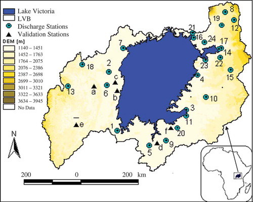
Fig. 1 Lake Victoria Basin (LVB) showing locations of the discharge stations and validation stations (see Table 1 for details).

Unfortunately, data limitation of the historical time series in the LVB is a major setback to such a study. Over reasonable areas of the LVB, either the catchments are ungauged, or gauged stations are not continuously operational due to poor maintenance. This data limitation creates high uncertainty in the calibration of the appropriate evd. One of the approaches that can be used to partly solve the data limitation problem is regionalization through regression models (as the form in equation (2)), which are constructed from basin characteristics or climatic variables. Such approach was used by the United States Geological Survey (USGS) as summarized in Jennings et al. (1994). According to Smakhtin (2001), the most commonly used basin and climate characteristics include: catchment area, mean annual precipitation, channel and/or catchment slope, stream frequency and/or density, percentage of lakes and forested areas, various soil and geology indices, length of the main stream, catchment shape and watershed perimeter, and mean catchment elevation. Regression models using a number of catchment characteristics were also developed in streamflow analysis in Australia by Nathan and McMahon (1991, 1992). Garcia-Martinó et al. (1996) developed statistical models for streamflow estimation in Puerto Rico using selected basin characteristics including drainage density, the ratio of the length of tributaries to the length of the main channel, the percentage of drainage area with northeast aspect, and the average weighted slope.

This study implemented and tested a regionalization attempt in statistical analysis of high flows to derive QDF relationships. The analysis is based on 24 selected catchments in the LVB, which is part of the Upper White Nile basin. To enhance the statistical accuracy and efficiency of the study findings and/or conclusions, emphasis was put on long-term discharge time series, preferably longer than 25 years. Six additional catchments with more limited flow records were considered for the validation of the regional QDF model (see Table 1).

Figure 1 shows the locations of the discharge measurement stations used in this study and Table 1 shows, for the selected catchments, some characteristics including flow record lengths, mean flow, locations and the physiographic characteristics.

Table 1 Details of selected stations and their characteristics. Long.: Longitude Lat.: Latitude SL: Slope

No.	Selected catchments	Station ID	Area (km^2)	Data length		Location		Point SL (%)	Mean flow (m^3 s^−^1)
				From	To	Long. (deg.)	Lat. (deg.)
1.	Biharamulo	***	1981	1950	2004	31.29	2.62	1.40	18.2
2.	Bukora	81270	8392	1951	1976	31.48	−0.85	0.46	3.1
3.	Grumeti	5F3	13363	1950	2004	33.94	−2.06	1.60	11.2
4.	Gurcha-migori	1KB05	6600	1950	2004	34.20	−0.95	2.00	57.7
5.	Isanga	114012	6812	1976	2004	32.77	−3.21	0.30	29.7
6.	Kagera	58370	54260	1950	1994	31.43	−1.29	3.00	266.3
7.	Katonga	100006	15244	1950	1975	31.95	−0.09	0.76	5.1
8.	Koitobos	1BE06	813	1949	1975	35.09	0.97	2.15	3.2
9.	Magogo-maome	113012	5207	1950	2004	33.15	−2.92	0.40	7.8
10.	Mara	107072	13393	1950	2003	34.56	−1.65	2.00	37.3
11.	Mbalangeti	111012	3591	1950	2004	33.86	−2.22	0.60	4.3
12.	Moiben	1BA01	188	1953	1990	35.44	0.80	2.13	1.3
13.	Nyakizumba	100005	359	1950	1987	30.08	−1.32	4.01	4.7
14.	Nyando	1GD01	3652	1962	2001	35.04	−0.10	5.00	20.3
15.	Nyangores	1LA03	4683	1963	1993	35.35	−0.79	1.02	8.3
16.	Nzoia	1EF01	12676	1974	1999	34.08	0.13	2.01	115.4
17.	Ogilla	1GD03	2650	1970	1996	34.96	−0.13	1.37	16.5
18.	Ruizi	100004	2070	1970	1998	30.65	−0.62	0.29	3.8
19.	Sergoit	1CA02	659	1959	1990	35.06	0.63	2.46	2.3
20.	Simiyu Ndagalu	5D1	1205	1970	1996	33.56	−2.63	0.50	11.8
21.	Sio	1AH01	1450	1958	2000	34.15	0.38	1.03	11.4
22.	Sondu	1JG01	3508	1950	1990	35.01	−0.39	2.30	43.3
23.	South Awach	1HE01	3156	1950	2004	34.54	−0.47	0.82	6.0
24.	Yala	1FG01	3351	1950	2000	34.51	0.09	2.30	37.3
Validation stations
(a)	Kagera Nyakanyasi	5A13	48427	1970	1978	31.20	−1.18	1.97	228.8
(b)	Ngono kalebe	5A3	1161	1970	1978	31.67	−1.41	0.81	15.3
(c)	Ngonokyaka/Bukoba	5A1	3200	1978	1989	31.60	−1.23	0.47	23.0
(d)	Pambani Mabuki Bridge	113022	1595	1970	1981	33.11	−2.97	1.11	2.33
(e)	Ruvuvu Mwendo	5A16	10970	1970	1977	30.56	−2.47	2.18	103.8
(f)	Simiyu Mwanza road	5D3	10200	1990	2001	33.45	−2.59	0.58	26.9

*** Station ID missing.

2 METHODOLOGY

2.1 QDF modelling

The extreme value analysis and QDF modelling are based on nearly independent extremes (peak values) extracted from daily full time series. This is done using independence criteria based on threshold values for the time difference between two successive independent peaks, the ratio of the minimum value between the two peaks to the peak value, and the peak height; see Willems (2009) for details on the method.

Prior to the extraction of the extreme values from the full time series for each of the selected stations, an n-day moving averaging window was passed through the series. Aggregation levels of 1 day up to 1 year were considered. This is the range covered by multipurpose applications (e.g. agricultural, irrigation, power plants, domestic water supply, pollution etc.). To come up with the amplitude–duration–frequency relationships, for the selected range of aggregation levels, extreme value analysis was carried out and the suitable evd was selected. To enable an adequate selection of the most optimal threshold level, and to avoid systematic over/under-estimation in the tail of the distribution, quantile plots or Q-Q plots were considered. The principle of calibrating the evds by a weighted linear regression in the Q-Q plot suggested by Csorgo et al. (1985) and Beirlant et al. (1996), and used by Willems et al. (2007), Taye and Willems (2011), Onyutha (2012) and Onyutha and Willems (2013), was adopted for this study. The extreme value index γ_evd (or k = −γ_evd), which is a parameter in the generalized extreme value (GEV) distribution of Jenkinson (1955), or the generalized Pareto distribution (GPD) of Pickands (1975), enables identification of the shape of the evd. The class of the GEV distribution or GPD is identified as heavy tail (when γ_evd > 0 or k < 0), normal tail (when γ_evd = k = 0), or light tail (when γ_evd < 0 or k > 0). The weighting factors proposed by Hill (1975) were considered.

Figure 2 shows examples of calibrated evds as linear regression lines in exponential Q-Q plots. As explained in Beirlant et al. (1996) and Willems et al. (2007), linear upper tail behaviour as in Fig. 2 means that the tail can be described by an exponential evd (which is a special case of the GPD with zero shape parameter):

(1)

Fig. 2 Observations (o) in exponential Q-Q plots of daily discharges for high flows in: (a) Nyando River (station 1GD01) and (b) Nzoia River (station 1EF01). □ denotes the selected optimal threshold; and the regression line is the calibrated evd.

where Q_T is the discharge (m³ s^-1) of return period, T (years); T₀ is the return period equal to or higher than that of the threshold event; Q_T0 is the discharge (m³ s^-1) of return period, T₀ (years); and β is the slope (scale parameter) of the exponential evd.

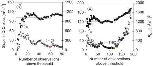
Due to the fact that high fluctuations occur in the slope of the Q-Q plots (e.g. in Fig. 3) for high thresholds due to randomness of the dataset, the slope estimates for these high thresholds have high statistical uncertainty. Instead, for very low thresholds, the slope estimates might result in pronounced bias (see the increasing slope on the right-hand side of Fig. 3(b)). The selection of optimal threshold values x_t above which the distributions are calibrated was ensured to be at points above which the mean squared error (E_MS) of the linear regression is minimal, i.e. within nearly horizontal sections in the plot of the slope vs the number of observations above the threshold. For the examples of the daily flows of Nyando River (station 1GD01) and Nzoia River (station 1EF01), the optimal thresholds are determined as the flow values with threshold ranks t = 59 and t = 118 (i.e. the 59th and 118th highest flow values) as shown in Fig. 3(a) and (b), respectively. A linear tail behaviour in the exponential Q-Q plot was obtained towards the higher Q values.

Fig. 3 Daily discharges of (a) Nyando River (1GD01) and (b) Nzoia River (1EF01). Left vertical axis, ♦: Hill-type estimation of slope in the exponential Q-Q plot; right vertical axis, ◊: mean squared error (E_MS) of Hill-type regression in the exponential Q-Q plot; □: selected optimal threshold.

Next, after carefully selecting, in a consistent way, the optimal thresholds for the different aggregation levels, the parameters of the evd were calibrated and the relationship between the model parameters and the aggregation levels was analysed, as in Onyutha and Willems (2013). To derive smooth mathematical relationships, small but acceptable modifications were made to the model parameters. The parameter/aggregation level relationships, together with the analytical description of the evd, finally constituted the QDF relationships, as is shown in Section 2.2.

2.2 Parameterization

To capture the differences in the characteristics of the QDFs for the selected stations, several parameters were derived, as discussed below.

2.2.1 Parameter α_s

For catchments a, b, c, …, z and a particular T, we can have corresponding flow quantiles Q_a[T], Q_b[T], Q_c[T], …, Q_z[T]. If a point of reference, say flow quantile Q_R[T], is selected, the differences (Q_a[T] – Q_R[T]), (Q_b[T] – Q_R[T]), (Q_c[T] – Q_R[T]), …, (Q_z[T] – Q_R[T]) define parameters α_a[T], α_b[T], α_c[T], …, α_z[T], respectively. Parameter α_s indicates by how much the extreme values, i.e. flow quantiles, described by a QDF relationship have to be brought onto common curve for the region; in other words, it is a scaling measure. This parameter quantifies the site to site variation in hydrological events. This variation can be ascribed to the size of the catchment, the local climate, e.g. rainfall statistics, the catchment’s land use, its topography, etc. The higher the value of parameter α_s, the higher are the flow extremes. This means that parameter α_s controls the magnitude of the runoff values. However, it is important to note that the basis for the choice of the reference curve to obtain parameter α_s is subjective. In this study, α_s was taken as the flow quantile for the 1-day aggregation level for all the selected catchments as illustrated in Fig. 4. With increase in the return period, the value of α_s increases.

Fig. 4 Parameters characterizing the peak flow QDFs for (a) parameter γ and (b) parameter α_s.

2.2.2 Parameter γ

This is the slope of a QDF curve for a particular return period (see Fig. 4). The value of γ is negative for high-flow QDFs. It defines how strong the temporal variability in river flows is reduced by temporally aggregating the series. It can be taken to be an indicator of the dryness or duration of dry spells of the catchment under study. A more negative γ value indicates higher intermittency in the daily flows, i.e. the existence of longer dry spells or stronger wet-dry variations, while a less negative value of γ indicates higher temporal homogeneity in the streamflow of the catchment under consideration. Hence γ also reflects the runoff variability over the catchment.

2.2.3 Parameter β

This is the slope of the evd in an exponential Q-Q plot (see equation (1)). Note that for the exponential evd, the relationship between the extreme flow quantile and the reduced variate (taken here to be the log-transformed return period) is linear. This means that for the same difference in log-transformed return periods (or log-frequency range), the same value for the difference between any two successive T-year curves on QDF relationship is obtained. It is parameter β that determines how far apart the T-year curves for any selected successive return periods on QDF relationships can be. In this paper, β was considered at the 1-day aggregation level in the QDF relationships. A higher value of β means higher extreme flow variations. It is important to note that, when the scaling parameter α_s is known for a given return period, the scaling parameter can be computed for other return periods using β.

2.3 Analysis of correlative relationships between the QDF parameters

The relationships between the parameters derived from the theoretical QDFs were examined. The coefficient of determination, R² was used to judge the goodness-of-fit for the correlative relationships. The main idea here is that, in the case of the existence of some correlative relationships between the QDF parameters, advantage can be taken of the interdependency to avoid the regional regression models being developed for each parameter.

2.4 Regression models

In support of the regionalization approach, a search is done for physiographic or hydroclimatic characteristics that explain the variations in the parameters characterizing the QDF relationships of the selected catchments. If such explanatory characteristics can be found, they can be used as predictors in regression models of the QDF parameters α_s, γ and β. These models would make it possible for ungauged catchments to estimate their QDF relationships. According to Downer (1981), development of a better understanding of the physical factors affecting the streamflow can help to enhance the accuracy of regression models. The most important step in the build-up of the regional regression models entailed the careful selection of the predictor variables. In this study, the following catchment characteristics were considered: catchment area (A_R, km²), mean point catchment slope (S_L, %), mean annual rainfall (R_AM, mm), mean annual potential evapotranspiration (E_MAT, mm), closest distance to the Lake Victoria shoreline (D_L, km), the mean point elevation (E_LEV, m a.s.l.), and the aspect (A_SP, -). The S_L and E_LEV were selected because they determine the catchment response to runoff, while D_L captures the hydroclimatic influence of Lake Victoria on the surrounding catchments in the study area. Catchment rainfall intensity determines the magnitude of hydrological extreme events. Parameter A_SP reflects the direction of catchment runoff, i.e. the bearing of Lake Victoria from a particular catchment in question. The values of S_L, A_SP and E_LEV were estimated from the 90 m × 90 m digital elevation model (DEM) by averaging 100 randomly selected points in the catchment area upstream of a given measurement station. The Hole-filled DEM derived from the USGS/NASA (Jarvis et al. 2008) and processed by the International Centre for Tropical Agriculture (CIAT-CSI-SRTM) using interpolation methods described by Reuter et al. (2007) was used in this study. In a trial-and-error procedure, jointly for all the selected catchments of the study area, the correlative relationships of α_s, γ and β with the physiographic and/or hydroclimatic characteristics were examined through scatter plots. Multivariate regression models entailing the multiplicative relationships were tested. The multiplicative model takes the following form:

(2)

where ρ is the parameter to be predicted; a_j are regression coefficients, j = 0, 1, 2, …, n; and P_i is the predictor, i = 0, 1, 2, …, n.

Such multiplicative relationship was also considered by Stedinger et al. (1993) for the prediction of flood quantile estimates based on physiographic and climate characteristics. An expression of the form of equation (2) was also included in the Urban Drainage Design Manual of the Federal Highway Administration (FHWA 1996) for estimating peak flows from basin characteristics. In this study, the multiplicative combination with the least number of physiographic and/or hydro climatic characteristics giving partial correlation of at least 0.4 with a particular parameter of the QDF relationship was adopted as a predictor.

In the calibration procedure, all the 24 selected catchments were jointly used for a selected return period. During the calibration, the evaluative ‘goodness-of-fit’ analysis was both graphically and statistically done. Statistically, so as to achieve a high value of R², adding more variables might be an option one would wish to undertake irrespective of whether the added variables are relevant or not. This trick is not encouraging but rather misleading, and, consequently, an adjusted R² (Ȓ²) was used in this study since it considers some punitive measure attached to addition of more variables. Out of the various formulae outlined by Snyder and Lawson (1993) and Yin and Fan (2001), which shrink R² based on the number of predictors (v), sample size (n), and the obtained effect (R²) as an initial estimate of the population effect, Leach and Henson (2007) empirically evaluated the reporting of adjusted effect sizes (e.g. adjusted R²) in published multiple regression studies. They identified the types of corrected effects reported, and found that, out of the several adjusted R² formulae, the formula of Ezekiel (1930), as expressed in equation (3), provided the most conservative correction for sampling error.

The Ezekiel (1930) formula, which can reasonably be confused with that of Wherry (1931), is actually a modification of that in Ezekiel (1929). The Ezekiel (1930) formula given in equation (3) was used in this study:

(3)

where Ȓ² is the adjusted R²; and R² is the coefficient of determination.

Statistical goodness-of-fit results of the calibrations were also evaluated using the model efficiency coefficient (E_F). The popular efficiency coefficient of Nash and Sutcliffe (1970), given by equation (4), is a dimensionless and scaled version of the mean squared error (E_MS) and varies from 1 (indicating the best model performance) to negative infinity.

In a trial-and-error procedure, the regression parameters were first manually adjusted until the highest possible value of Ȓ² was achieved. In a fine-tuning step, the optimization technique of E_MS minimization was adopted. At this point, the computed standard error of regression estimates (S_e), which is actually the standard deviation of the predicted values of γ, was expected to be at its minimum.

2.5 Uncertainty and analysis of errors

After calibration, validation of the regression models was conducted based on six discharge measurement stations with short records of data (see Table 1). In this validation step, model performance was evaluated based on the model bias (B_ias) and the root mean square of the model residual error (E_RMS). Considering i to be the rank of the selected aggregation levels of the study (i = 1 for the lowest i.e. 1 day), H the number of aggregation levels, M_p,i the theoretical quantile at i, M_e,i the empirical quantile at i, and the mean of theoretical quantiles, the mean of values obtained from the expression (M_p,i – M_e,i) as a percentage of M_e,i for i = 1 to H is considered the average percentage bias (equation (5)). For an ideal model, the B_ias (%) is equal to zero and the model is said to be unbiased. The overall differences between M_e,i and M_p,i values for each catchment were also evaluated in terms the relative root mean squared error, E_RMS (equation (6)).

(4)

(5)

(6)

Since there were no empirical values in the QDFs for return periods higher than the length of the available flow series, the goodness-of-fit of flow quantiles had to be validated for the lower return periods of 5, 10, 15, 20 and 25 years. Using the empirical and theoretical daily discharges from the QDF relationships of all the selected stations, the B_ias (%) and E_RMS (m³ s^-1) for the aforementioned return periods were evaluated using equations (5) and (6), respectively.

2.6 Validation of regression models

Ideally, T-year curves are to be parallel to each other on QDF relationships. This means that the deviations of parameter γ for the selected T-year curves on QDF relationships are expected to be minimal. Estimating QDF relationships in ungauged catchments taking into account the interdependency of the parameters of a QDF can be carried out using the following steps:

1. estimate parameter γ for a return period of 5 years using equation (2);

2. determine parameter β from its relationship with the estimated parameter γ;

3. determine parameter α_s for a return period of 5 years from its relationship with β or γ; and

4. use the estimated parameters α_s and β to derive QDF relationships for return periods longer than 5 years (equation (1)).

3 RESULTS AND DISCUSSION

3.1 QDF models

Figure 5 shows examples of the QDF relationships obtained from compiling the exponential evd calibration results for river flows aggregated over time scales of 1, 3, 5, 7, 10, 30, 45, 60 and 90 days, after parameterization of the QDF relationships. Up to the length of the available time series, empirical quantiles were derived as well. Because the lengths of the available river flow series were all more than 25 years, empirical T-year events are only shown for curves up to 25 years in Fig. 5. For higher return periods, due to the randomness involved in the empirical data, the empirical quantiles can be far more inaccurate in comparison with the theoretical quantiles. Differences between the empirical and theoretical quantiles can, for the higher return periods, also be explained by the influence of river flooding i.e. the difference between the river discharges and the catchment rainfall-runoff discharges.

Fig. 5 Calibration results of peak flow QDF relationships for: (a) Nzoia River (station 1EF01) and (b) Nyando River (station 1GD01). Legend: e.g. T₅ denotes T-year curve for T = 5 years.

Figure 6 shows the graphical goodness-of-fit of the flow quantiles after calibration of the evds for daily aggregation level; for return periods of 5, 10 and 25 years. Considering the full range of aggregation levels, low values of B_ias (%) and E_RMS (m³ s^-1) were realized for the calibrated T-year flow estimates as seen in Table 2. This means that, the fittings between empirical and theoretical points defining QDF relationships before parameterization were highly acceptable.

Fig. 6 Evaluation of QDF calibration results for daily high flows of all selected catchments for return periods of 5 (◊), 10 (*) and 25 (●) years.

In practice, for design of hydraulic structures such as along sewer and river systems, bridges and culverts, return periods between 5 and 100 years are used. Higher return periods around T₁₀₀ are used mainly for flood plain development, and medium-sized flood protection works. Although T₅₀₀ is rarely used in designs, it was in this study used for the assessment of the reliability of the projected QDF discharges for extreme conditions through extrapolation of the evd.

Table 2 The overall average B_ias (%) and E_RMS (m³ s^-1) for the calibrated T-year flow quantiles considering the full range of aggregation levels.

	T5	T10	T25
Bias (%)	−0.38	−0.58	−0.78
ERMS (m^3 s^-^1)	4.93	16.16	19.33
EF (-)	0.995	0.994	0.993

3.2 Relationships between the QDF parameters

Figure 7 indicates that, parameters α_s, γ and β all depend on each other. The following relationships were deduced:

(7)

(8)

(9)

This dependency between the QDF parameters means that they all depend on the magnitude of the temporal variability in streamflow. For stations with higher temporal variability (stronger differences between low and high flows), parameter γ indicates a higher slope (more negative values; because of stronger differences between short-duration values and longer duration values), parameter α_s will be higher because extremes will be higher for small aggregation levels, and parameter β will be higher because of higher difference between low and high extremes. The parameters α_s and γ used to obtain Fig. 8 and equations (7)–(9) were picked from a return period of 5 years. Similar plots were however made with all the selected return periods of the QDF relationships. The values of R² in the regression between QDF parameters were noted to reduce with increase in the return periods due to the higher uncertainty in extreme value analysis for higher return periods.

Fig. 7 Relationships between the QDF parameters α₅, γ₅ and β.

3.3 Relating QDF parameters to physiographic and hydroclimatic catchment characteristics

As shown in Table 3, the R² values of the regression models between the QDF parameters and physiographic or hydroclimatic catchment characteristics are low when individual characteristics are considered as single predictor. However, the correlative relationships are largely enhanced when different catchment characteristics are combined through multiplicative models of equation (2). As shown in Table 4, the highest R² values were obtained when A_R, and S_L are combined, such as when [A_RS_L] or [A_RS_LR_AM] are used as predictor variable. Fig. 8 shows the 5-year QDF parameters versus [A_RS_L].

Table 3 R² for relationships between the QDF parameters α_s, γ and β and individual possible predictors; α_s and γ are for a return period of 5 years.

	RAM	AR	SL	ELEV	DL	ASP	EMAT
αs	0.203	0.156	0.083	0.042	0.071	0.276	0.042
γ	0.220	0.072	0.091	0.007	0.065	0.203	0.110
β	0.140	0.007	0.179	0.004	0.097	0.171	0.065

Table 4 R² for relationships between the QDF parameters α_s, γ and β and possible combined predictors; α_s and γ are for a return period of 5 years.

	RAM. AR	RAM. SL	AR. SL	ELEV.ASP	RAM.DL	SL.DL	AR. SL.RAM	AR. SL. EMAT
αs	0.206	0.160	0.550	0.158	0.048	0.027	0.614	0.438
γ	0.098	0.193	0.397	0.082	0.035	0.020	0.444	0.307
β	0.017	0.262	0.484	0.065	0.075	0.018	0.527	0.235

Table 5 shows values of R² for the relationships between QDF parameters and the predictor variable taken as [A_RS_L] or [A_RS_LR_AM] with and without scaling exponents. For the models with scaling exponents, the final values of R² shown in Table 5 were again obtained after application of E_MS minimization to obtain optimal sets of the regression coefficients. The difference in R² values obtained for the models with and without scaling exponents is small. Eventually, model a₀(A_RS_L)^a1 was selected because it has the lowest number of parameters among the models with the highest R² values.

Table 5 R² for relationships between the QDF parameters α_s and γ and combined predictors with increase in return period.

	T5	T10	T25	T100	T500	T5	T10	T25	T100	T500
Model = (AR. SL)						Model = (AR. SL. RAM)
αs	0.550	0.524	0.506	0.483	0.308	0.614	0.585	0.565	0.539	0.493
γ	0.446	0.440	0.420	0.410	0.400	0.477	0.474	0.473	0.472	0.473
Model = a0.(AR. SL)^a^1						Model = a0. (AR. SL. RAM) ^a^1
αs	0.545	0.543	0.527	0.537	0.548	0.550	0.582	0.588	0.604	0.561
γ	0.506	0.551	0.561	0.568	0.523	0.550	0.582	0.588	0.604	0.561
Model = a0.AR ^a^1. SL ^a^2						Model = a0.AR ^a^1. SL ^a^2. RAM ^a^3
αs	0.620	0.618	0.602	0.612	0.623	0.655	0.646	0.615	0.581	0.534
γ	0.518	0.570	0.581	0.589	0.539	0.559	0.591	0.598	0.610	0.565

Fig. 8 Relationships of the combined physiographic characteristic [A_R.S_L] with QDF parameters (a) α_s and (b) γ.

The careful combination of predictors is a plausible approach because it avoids overfitting resulting from multicollinearity and overparameterization in the regression model. The calibrated regional regression models for T = 5 years can be seen in Fig. 9 and Table 6. From Table 5 it can be seen that the values of the R² of the regression models reduce with increase in return periods. This again is due to the uncertainty boost in extreme value analysis as return periods increase.

Table 6 Regional regression models for QDF parameter γ.

Model	a0	a1	Ȓ^2	EF (-)	Se (m^3 s^-^1) d^-1	ERMS (m^3 s^-^1)
a0(ARSL)^a^1	−2.88E-01	5.03E-01	0.4834	0.5258	0.0463	0.2170

3.4 Regression model

Table 6 shows the regional regression model for the QDF parameter γ using the combined characteristic in the form a₀(A_RS_L)^a1. The calibrated regional regression models were evaluated both graphically (Fig. 9) and statistically (Table 6). The computed standard deviations (S_tdev) and standard error of regression estimates S_e, reflect the total uncertainty in the regression models. This uncertainty might be due to the incomplete model structure as well as the uncertainty in the statistical extreme value analysis and the river flow measurement errors.

Fig. 9 Evaluation of the calibration results of the regional regression model.

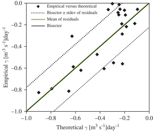
Since parameter γ was found to be correlated to both parameters α_s and β, the regression model was developed only for γ = 5 years so that α_s and β can be estimated from their dependency relationship with γ.

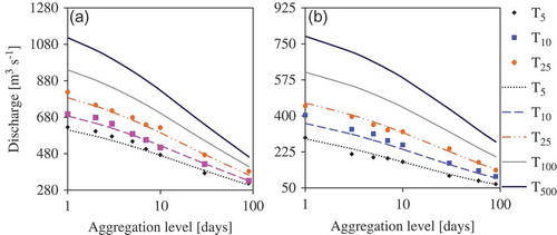
The examined variation of the QDF parameters with return period can be seen to follow power curves tending to asymptotic behaviour with very high return periods (see Fig. 10). The shapes of these curves were found to remain similar for all the catchments. The parameters α_s and γ vary smoothly with changing return period. The magnitude of parameter γ decreases as the return period increases; the reverse is true for parameter α_s(Fig. 10).

Fig. 10 Variation of QDF parameters (a) γ and (b) α_s with return period. ●: Nyando River (station 1GD01); □: Yala River (station 1FG01).

3.5 Spatial variations in the QDF parameters and hydroclimatic variables

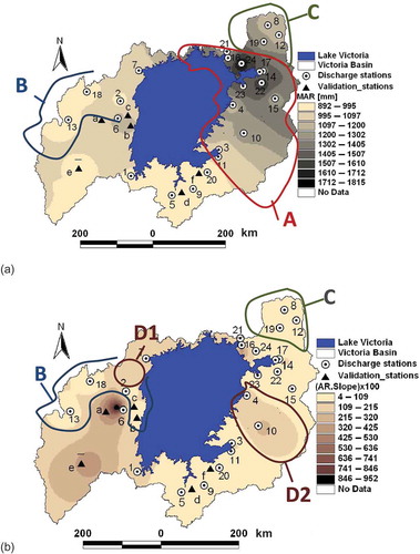
Figures 11 and 12 show the spatial variation of QDF parameters using R_AM and A_RS_L. These maps were obtained by surface interpolation (kriging method) of the standardized QDF parameters β and α_s based on the 30 catchments. The spatial maps for R_AM and A_RS_L were obtained using observations from meteorological stations within and around the study area.

For ease of visualization of the similarities between maps (a) and (b) of Fig. 11, areas with similar patterns have been encircled; this can be seen in the northeastern (C), eastern (A) and northwestern parts (B) of the basin. Of course, due to low spatial density of the network of stations, there are local influences from individual stations. For that reason, spatial similarities should not be compared at the level of individual stations but for larger areas. One possible solution to overcome this problem is to filter out the influence of local stations using stronger spatial smoothing, but this was not feasible due to the low resolution of stations in some regions, such as the southwestern region around station e. There are some local inconsistent values which indicate that more reliable QDF fittings to yield consistent hydrological parameters such as α_s, γ and β for a given region can be deduced only when there are more discharge stations with available flow observations. The 24 discharge stations considered for the study might have been less than required to obtain clear regional (spatial) variations of the parameters derived from the QDF relationships.

Fig. 11 Spatial maps showing regional differences in terms of: (a) β, and (b) α_s for T = 5 years.

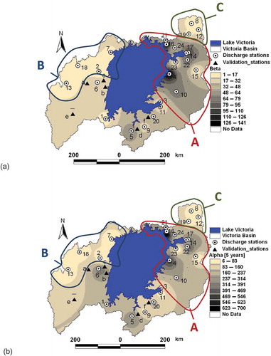
Region A in Figs 11 and 12(a) shows higher α_s, β and γ values in the areas close to Lake Victoria, whereas the regions B and C show lower values. The higher values in region A are explained by the higher rainfall extreme intensities in that region, as shown in the Nile basin regional extreme value analysis by Nyeko-Ogiramoi et al. (2012). These higher intensities are also reflected in the higher R_AM values for that region (Fig. 12(a)). In the south of region A, around stations 4 and 10, the R_AM values are lower but the QDF parameters α_s, β and γ remain high because of the higher A_RS_L values for these stations (sub-region D2, Fig. 12(b)). For the same reason, a similar pattern can be obtained in the northwestern area between stations 2 and 7 (sub-region D1, Fig. 12(b)). Also, the higher α_s value for station 6 is due to the higher catchment area. The lower QDF parameter values for encircled regions B and C are explained by both lower rainfall volumes and lower A_RS_L values. The stations in the south, such as stations 5, 9, 20, d and f, also have low R_AM and A_RS_L values, but, due to the higher E_MAT for that region (not shown), β and γ values are lower than that of regions B and C.

Fig. 12 Spatial maps showing regional differences in terms of: (a) R_AM, and (b) A_RS_L.

3.6 Validation of regional QDF models

Due to the fact that the validation stations were characterized by short data records (less than 12 years), the regional regression models were validated for return periods of 5, 10, 15, 20 and 25 years. This is because the short data records may cause high uncertainty in the statistical analysis of extreme events if used to estimate QDF relationships for very high return periods e.g. 100 or 500years. Table 7 shows the overall B_ias (%) and E_RMS (m³ s^-1) in the QDF estimates. The overall B_ias and E_RMS values increase with increasing return period (see also Fig. 14).

Table 7 The overall B_ias (%) and E_RMS (m³ s^-1) for T-year flow estimates computed as average value considering all six validation stations and considering the full range of aggregation levels.

T (years)	5	10	15	20	25
Bias (%)	−2.01	14.98	19.96	22.96	27.04
ERMS (m^3 s^-^1)	29.61	44.91	63.76	79.83	102.95

From Table 7 it can be seen that for a return period of 5 years, the validation result is reasonably well. However, for higher return periods, significant overestimations are found. This might be due to uncertainties in both the empirical and the theoretical flow quantiles, due to the uncertainty in the statistical extreme value analysis, and the flow measurement errors. There might also be the most important reason that the validation periods are limited in their length; hence the empirical flow values might be biased from the longer term values due to the decadal or multi-decadal climate oscillations, as shown in Taye and Willems (2011). Figure 13 shows the mean temporal variability (computed using a time slice of 5 years) for mean of annual maxima of river flows (R_AMF) of all the selected catchments of LVB in Table 1. The oscillation pattern of Fig. 13 was calculated using the quantile anomaly indicator, the details of which are discussed in Ntegeka and Willems (2008) and Willems (2013). Since the construction of QDF relationships is dependent on the periods used for the statistical analysis, the QDF quantiles obtained are respectively higher and lower during the oscillation highs (OHs) and lows (OLs) in comparison with the use of long record data. They may lead to biases in the QDF quantiles when they are based on short data records. From Fig. 13, it is shown that OHs in the mean of R_AMF of LVB occurred in the mid-1960s, the period between the late 1970s and early 1980s, and the 1990s. The OHs of the mid 1960s and the 1990s were significant at the 5% level of significance. The OLs were in the 1970s and the mid-1980s. It is also shown from Fig. 13 that there was a steadily increasing trend from 1970 to 2000 at a rate of 0.909% per year. If such temporal variations are significant, the applicability of the regional regression models may be lowered unless bias correction is applied in order to correct the QDF quantiles to account for the longer term flow variations. This can be done based on the anomaly indicator shown in Fig. 13, as demonstrated by Taye and Willems (2011).

Fig. 13 Temporal variability in the mean of annual maxima of LVB river flows for the period 1955–2000 using a time slice of 5 years.

The significant overestimations in the validation result might also be the influence of flooding. It also might be due to the uncertainty in the developed regional regression models, which have limited capacity to capture the site to site hydrological variations. If more stations with available data would become available, most likely the accuracy of the regional models could be largely improved. Another reason for the overestimations in the QDF estimates is that the predictors used in the regional regression models, i.e. A_R and S_L, are static in nature and may not adequately capture the changes in streamflow regimes in time. Improved regional regression models might also be obtained from regional regression analysis using data from hydroclimatic variables such as rainfall and evapotranspiration at smaller time steps, e.g. at daily resolutions.

Figure 14 shows evaluation of regional regression models for selected return periods. By considering the E_RMS as the measure of uncertainty in the QDF estimates, it can be seen that the E_RMS increases with increasing return periods (Fig. 14). For all the return periods considered, the highest and the lowest E_RMS values were obtained for Kagera Nyakanyasi and Ngono Kalebe (i.e. the largest and the smallest catchments) respectively. The size of the catchment and the consequent order of magnitude of the streamflows thus have a strong influence on the accuracy of the QDF estimates.

Fig. 14 Evaluation of QDF regional models for return periods of 5, 10, 15, 20 and 25 years: (a) B_ias (%), and (b) E_RMS (m³ s^-1) of T-year flow estimates.

4 CONCLUSIONS

This paper has provided a means of constructing estimates of QDF relationships for the hydrological extremes of ungauged catchments in the LVB for a number of applications including irrigation, hydropower supply and water supply, to assess the water management requirements in terms of cumulative volumes of water available during high flows. This can be done based on specific aggregation levels or return periods depending on the application. Twenty four selected catchments in the study area were used to model and characterize QDF relationships so as to capture their slopes (γ), tail behaviour (β) of the evd and scaling measures (α_s). The QDF parameters α_s, γ and β were found to depend on each other. Their spatial variability could be ascribed to site to site differences between the catchments with respect to the hydroclimatic (rainfall, evapotranspiration) and physiographic characteristics such as catchment area and slope. To explain the regional difference in the QDF parameters from these physiographic characteristics, regional regression models were obtained based on combined multiplicative relationships. Catchment area, slope and mean annual rainfall were found to have the highest correlations with the QDF parameters. The multiplicative combination of these three characteristics was found to present the highest correlative relationships with the QDF parameters with the R² values of 0.61, 0.44 and 0.52 for parameters α_s, γ and β, respectively. For the multiplicative combination of area and slope, the R² values only reduced slightly. The regression model a₀(A_RS_L)^a1 was selected because it has low number of parameters but high R² value. Application of scaling exponents to the individual catchment characteristics in the regression model did not show significant improvement in the model performance. From the calibration results, E_RMS and B_ias for modelled vs observed flow quantiles were found to be 0.23 m³ s^-1 and 0.37%, respectively. The average percentage bias for all validation stations and aggregation levels considered is –2% and 27% for the lowest and highest return periods considered in the study, i.e. 5 and 25 years, respectively.

It should be noted that the physiographic characteristics used in the regression models are static and may not adequately capture the changes in streamflow regimes with time. In determining the relationships between the streamflow QDF statistics and the physiographic and hydroclimatic characteristics, mean annual rainfall data was used. It is however expected that, improved models might be obtained from rainfall volumes during the wet seasons, or from daily rainfall based extreme value analysis. In the update of the regional regression models, more discharge measurement stations with up-to-date data could be used to fine tune the interdependency between the QDF parameters, and also the correlative relationships between parameters α_s, γ and β and the physiographic or hydroclimatic characteristics. Another interesting study would be to determine the variability in parameters α_s, γ and β and examine if they are correlated with the trends in land use of the study area; this would help to deduce a quantitative measure in the variability pattern for the parameters α_s, γ and β with respect to the anthropogenic influence.

Disclosure statement

No potential conflict of interest was reported by the author(s).

Acknowledgement

The historical discharge data were obtained at KU Leuven from the database of the FRIEND/NILE project (http://www.unesco.org/new/en/cairo/natural-sciences/hydrology-programme/friendnile/ [accessed 10 September 2014]). The DEM used in this study was obtained online from the International Centre for Tropical Agriculture, CIAT-CSI SRTM website, http://strm.csi.cgiar.org/[accessed 30 November 2010].

ORCID

Patrick Willems http://orcid.org/0000-0002-7085-2570

Additional information

Funding

The research was linked to the FRIEND/NILE project of UNESCO and the Flanders in Trust Fund. Financial support was obtained from VLIR-UOS scholarship for Inter-University Master programmes, and an IRO PhD scholarship of KU Leuven, all in Belgium.

REFERENCES

- Beirlant, J., Teugels, J.L., and Vynckier, P., 1996. Practical analysis of extreme values. Leuven: University Press Leuven.
- Chow, V.T., Maidment, D.R., and Mays, L.W., 1988. Applied hydrology. New York, NY: McGraw-Hill.
- Csorgo, S., Deheuvels, P., and Mason, D., 1985. Kernel estimates of the tail index of a distribution. The Annals of Statistics, 13, 1050–1077. doi:10.1214/aos/1176349656
- Downer, R.N., 1981. Low-flow studies for Vermont—a prognosis for success. In: Hydro power and its transmission in the Lake Champlain Basin. Proceedings of the eighth annual Lake Champlain Basin environmental conference, 43–51.
- Ezekiel, M., 1929. The application of the theory of error to multiple and curvilinear correlation. American Statistical Association Journal, 24, 99–104.
- Ezekiel, M., 1930. Methods of correlational analysis. New York, NY: John Wiley and Sons.
- Federal Highway Administration, FHWA, 1996. Urban drainage design manual (SI), hydraulic engineering circular no. 22 (FHWA-SA-96-078). Washington, DC: US Department of Transportation.
- Garcia-Martinó, A.R., et al., 1996. Statistical low-flow estimation using GIS analysis in humid montane regions in Puerto Rico. Journal of the American Water Resources Association, 32 (6), 1259–1271. doi:10.1111/j.1752-1688.1996.tb03495.x
- Gichere, S.K., et al., 2013. Effects of drought and floods on crop and animal losses and socio-economic status of households in the Lake Victoria Basin of Kenya. Journal of Emerging Trends in Economics and Management Sciences, 4 (1), 31–41.
- Hill, B.M., 1975. A simple and general approach to inference about the tail of a distribution. The Annals of Statistics, 3, 1163–1174. doi:10.1214/aos/1176343247
- Jarvis, A., et al., 2008. Hole-filled seamless SRTM data V4, International Centre for Tropical Agriculture (CIAT) [online]. Available from: http://srtm.csi.cgiar.org [Accessed 30 November 2010].
- Jenkinson, A.F., 1955. The frequency distribution of the annual maximum (or minimum) values of meteorological elements. Quarterly Journal of the Royal Meteorological Society, 81 (348), 158–171. doi:10.1002/qj.49708134804
- Jennings, M.E., Thomas, W.O. Jr, and Riggs, H.C., 1994. Nationwide summary of US Geological Survey regional regression equations for estimating magnitude and frequency of floods for ungaged sites, 1993. US Geological Survey, Water Resources Investigations Report 94–4002, prepared in cooperation with the Federal Highway Administration and the Federal Emergency Management Agency, Reston Virginia.
- Leach, F.L. and Henson, K.R., 2007. The use and impact of adjusted R2 effects in published regression research. Multiple Linear Regression Viewpoints, 33 (1), 1–11.
- Nash, J.E. and Sutcliffe, J.V., 1970. River flow forecasting through conceptual models part I—a discussion of principles. Journal of Hydrology, 10, 282–290. doi:10.1016/0022-1694(70)90255-6
- Nathan, R.J. and McMahon, T.A., 1991. Estimating low flow characteristics in ungauged catchments: a practical guide. Melbourne: Department of Civil and Agricultural Engineering, University of Melbourne.
- Nathan, R.J. and McMahon, T.A., 1992. Estimating low flow characteristics in ungauged catchments. Water Resources Management, 6 (2), 85–100. doi:10.1007/BF00872205
- Nhat, L.M., Tachikawa, Y., and Takara, K., 2006. Establishment of intensity-duration-frequency curves for precipitation in the monsoon area of Vietnam. Annals of Disaster Prevention Research Institute Kyoto University, 49, 93–103.
- Ntegeka, V. and Willems, P., 2008. Trends and multidecadal oscillations in rainfall extremes, based on a more than 100-year time series of 10 min rainfall intensities at Uccle, Belgium. Water Resources Research, 44 (7), W07402.doi:10.1029/2007WR006471
- Nyeko-Ogiramoi, P.O., et al., 2012. An elusive search for regional flood frequency estimates in the River Nile basin. Hydrology and Earth System Sciences, 16, 3149–3163. doi:10.5194/hess-16-3149-2012
- Onyutha, C., 2012. Statistical modelling of FDC and return periods to characterise QDF and design threshold of hydrological extremes. Journal of Urban and Environmental Engineering, 6 (2), 132–148. doi:10.4090/juee.2012.v6n2.132148
- Onyutha, C. and Willems, P., 2013. Uncertainties in flow-duration-frequency relationships of high and low flow extremes in Lake Victoria basin. Water, 5 (4), 1561–1579. doi:10.3390/w5041561
- Pickands III, J., 1975. Statistical inference using extreme order statistics. The Annals of Statistics, 3, 119–131. doi:10.1214/aos/1176343003
- Reuter, H.I., Nelson, A., and Jarvis, A., 2007. An evaluation of void‐filling interpolation methods for SRTM data. International Journal of Geographical Information Science, 21 (9), 983–1008. doi:10.1080/13658810601169899
- Smakhtin, V.U., 2001. Low flow hydrology: a review. Journal of Hydrology, 240, 147–186. doi:10.1016/S0022-1694(00)00340-1
- Snyder, P. and Lawson, S., 1993. Evaluating results using corrected and uncorrected effect size estimates. The Journal of Experimental Education, 61, 334–349. doi:10.1080/00220973.1993.10806594
- Stedinger, J.R., Vogel, R.M., and Foufoula-Georgiou, E., 1993. Frequency analysis of extreme events. In: D.R. Maidment, ed. Handbook of hydrology. New York, NY: McGraw-Hill, 18.1–18.66.
- Taye, M.T. and Willems, P., 2011. Influence of climate variability on representative QDF predictions of the Upper Blue Nile Basin. Journal of Hydrology, 411, 355–365. doi:10.1016/j.jhydrol.2011.10.019
- Wherry, R.J., 1931. A new formula for predicting the shrinkage of the coefficient of multiple correlation. The Annals of Mathematical Statistics, 2, 440–457. doi:10.1214/aoms/1177732951
- Willems, P., 2009. A time series tool to support the multi-criteria performance evaluation of rainfall-runoff models. Environmental Modelling software, 24 (3), 311–321.doi:10.1016/j.envsoft.2008.09.005
- Willems, P., 2013. Multidecadal oscillatory behaviour of rainfall extremes in Europe. Climatic Change, 120, 931–944.doi:10.1007/s10584-013-0837-x
- Willems, P., Guillou, A., and Beirlant, J., 2007. Bias correction in hydrologic GPD based extreme value analysis by means of a slowly varying function. Journal of Hydrology, 338, 221–236.doi:10.1016/j.jhydrol.2007.02.035
- World Meteorological Organization, WMO, 2008. Hydrological data. In: Manual on low-flow estimation and prediction; Operational Hydrology Report No. 50, WMO-No.1029, Geneva: WMO, 138p.
- World Meteorological Organization, WMO, 2009. Management of water resources and application of hydrological practices. In: Guide to hydrological practices, Volume II, 6th ed.; WMO-No.168, Geneva: WMO.
- Yin, P. and Fan, X., 2001. Estimating R2 Shrinkage in multiple regression: a comparison of different analytical methods. The Journal of Experimental Education, 69, 203–224. doi:10.1080/00220970109600656