Novel information for source identification of local pumping and recharging in a groundwater system

Abstract

The aim of this paper is to solve the local pumping and recharging source identification problem by introducing a statistical technique, independent component analysis (ICA), into groundwater modelling. Such a problem suffers from limited observations in the field and is ill-posed. With the help of ICA, the observed head at monitoring wells is decomposed into a linear combination of head fluctuations caused by each source. The ill-posed problem is transferred into several independent well-posed ones. Moreover, the decomposed hourly head fluctuation, specially referred to as ‘characteristic pattern’, provides novel information on the type and distance of local sources. A hypothetical case to identify two local sources using two observation wells is presented, and the results show the accuracy and efficiency of the proposed method. The identified results are stable as long as the observation error is within a reasonable range. The characteristic pattern provides novel information, which can be widely used for source identification in the future.

Editor D. Koutsoyiannis; Associate editor Xi Chen

Résumé Le but de cet article est de résoudre le problème de l’identification d’une source locale de pompage ou de recharge par l’introduction de la technique statistique d’analyse de composante indépendante (ACI) dans la modélisation des eaux souterraines. Un tel problème souffre d’observations limitées et est mal posé. Avec l’aide de l’ACI, la piézométrie observée dans des ouvrages de surveillance est décomposée en une combinaison linéaire de fluctuations piézométriques causées par chaque source. Le problème mal posé est transformé en plusieurs problèmes indépendants bien posés. En outre, la fluctuation piézométrique horaire décomposée, dénommée «schéma caractéristique», fournit une information nouvelle sur le type et la distance des sources locales. Un cas hypothétique est présenté pour identifier deux sources locales à l’aide de deux puits d’observation et les résultats montrent la justesse et l’efficacité de la méthode proposée. Les résultats identifiés sont stables aussi longtemps que l’erreur d’observation est dans une fourchette raisonnable. Le schéma caractéristique fournit une information nouvelle qui pourrait être largement utilisée à l’avenir pour l’identification de sources.

Key words:

• independent component analysis
• characteristic pattern
• source identification
• groundwater modelling

Mots clefs:

• analyse de composante indépendante
• schéma caractéristique
• identification de source
• modélisation des eaux souterraines

1 INTRODUCTION

In the early days, water resources development focused on surface water, which constituted the majority of freshwater resources to meet basic human needs (Koutsoyiannis 2011). But with global population increases in recent years, water demand is also rising, and this coupled with climate change makes the surface water supply more unstable (Groisman et al. 2005). More countries are developing groundwater resources as supplementary solutions to water deficiency (Chiu et al. 2009, Safavi et al. 2010). Groundwater, which can easily be exploited by wells, has become a more convenient water supply source in the past few decades.

Around the world, groundwater is widely extracted (Llamas 2004, Don et al. 2005, Lee et al. 2005, Galloway and Burbey 2011). Before people became fully aware that pumping capacity had exceeded the recharge rate, land subsidence, saltwater intrusion and structure destruction had occurred, resulting in a considerable loss to society (Teatini et al. 2006, Galloway and Burbey 2011). Such substantial environmental impacts indicate that the exploitation of groundwater may not be more economical than investment in large surface water engineering projects (Koutsoyiannis 2011). Governments are quickly starting to manage the groundwater resource (Chou and Ting 2007, Calderhead et al. 2012, Nelson 2012).

The first step of groundwater resource management is to understand the entire groundwater system, and compile and analyse the system characteristics, including stratigraphic composition of lithology, aquifer stratification, hydrogeology, hydrological inflow and loss, groundwater level and water quality. Among these, lithology and stratification can be generally investigated by geological drilling and lithology analysis; hydrogeological parameters can be evaluated by in-situ pumping tests with given conditions (Sun 2005, Liu et al. 2009); groundwater level and water quality can be continuously monitored through a network of monitoring wells; and large-scale hydrological inflow and loss can be appropriately assessed through the water balance method. Currently, the most difficult variables to grasp and clarify are the time and space distribution of inflow and loss. In other words, local pumping and recharging source identification and quantity estimation remain a challenge for groundwater resource management (Porter et al. 2000, Rao 2006, Peng et al. 2010).

Local sources are difficult to identify because of limited information. The pumping and recharging at local sources can be viewed as a stimulation or perturbation to the groundwater system. In response, the groundwater level and water quality change. Such a change is the only data that can be observed and collected in the field through monitoring wells. The pumping and recharging is latent, meaning that they cannot be directly observed, and can only be estimated through indirect information. Based on groundwater level and water quality observations, as well as the correct understanding of the system, it should be possible to trace back the pumping and recharging sources.

Besides the limited information, another problem is that every observation is a mixed result of multiple sources rather than a single stimulation. In fact we cannot restrict it so that there is only one local source in the field. If there is only one source, the source location and its quantity can be easily estimated. This is because the number of observations will be far more than the number of unknowns. Unfortunately, the groundwater change due to individual sources cannot be known. Consequently, source identification in the past can only give a rough sketch of large-scale hydrology (Wittenberg and Sivapalan 1999, Ruud et al. 2004, Wang et al. 2005, Misstear et al. 2009), or can evaluate a few suspicious sources and related pumping or recharging rates using a large number of observed data in time and space (Aral et al. 2001, Tung and Chou 2004, Mahinthakumar and Sayeed 2005, Saffi and Cheddadi 2007, Ayvaz and Karahan 2008, Lin and Yeh 2008, Cheng et al. 2009, Saffi and Cheddadi 2010).

In reality, each pumping or recharging source has its own characteristic which makes them easy to distinguish from each other. The fundamental problem lies in that all observation data are blended, simultaneously influenced by two or more sources. It is difficult to use such data to infer the impact of any one individual source. The number of unknowns exceeds that of the observations, which makes the source identification problem ill-posed. Therefore, the basic concept of this research is to restore the observation first. The mixed signals should be returned to the original signals, that is, use signal processing techniques to achieve a situation of many monitoring wells simultaneously monitoring one signal local source. Then we can have more observations than unknowns and the ill-posed source identification problem can become a well-posed one. Such a situation is not possible to meet in the field. Unknown pumping and recharging sources are simplified into one, but the observation wells can be many, making source identification more likely to be correctly solved.

Based on this concept, we introduce a statistical technique, known as independent component analysis (ICA) (Jutten and Herault 1991), to analyse the groundwater head observations to extract the characteristics of sources. ICA has been applied in the signal processing area for years and achieved success in source separation and feature extraction (Hyvärinen and Oja 2000). ICA utilizes statistical theory and signal analysis techniques to decompose the observed mixed signals into independent components. In this paper, ICA is first applied to groundwater modelling combining with the groundwater simulation and optimization model to solve the local pumping and recharging source identification and quantity estimation problem. This new source identification procedure is tested in a designed virtual case to verify the correctness and feasibility of this method. Novel information on local pumping and recharging sources is also discovered through the case study, which can be widely used for source identification in the future.

2 METHODOLOGY

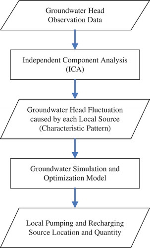
The methodology of local pumping and recharging source identification and quantity estimation is illustrated as a flow chart in Fig. 1. The first step is to collect observed groundwater head data; this is decomposed by independent component analysis (ICA) to obtain the groundwater head fluctuations caused by each local source. Each fluctuation is a special pattern, which we named the ‘characteristic pattern’. Each characteristic pattern contains the characteristics of each source and provides novel information for source identification. Every single characteristic pattern is put into the groundwater simulation and optimization model to best estimate one local source location and quantity. Repeat the simulation and optimization process by inputting different characteristic patterns, so that in the end, every local pumping and recharging source is identified. Details of the applied tools and each analysis step are described in order as follows.

Fig. 1 Flow chart of local pumping and recharging source identification and quantity estimation.

2.1 Groundwater head observation data

Groundwater head observations are obtained from monitoring wells located at adequate spatial coordinates. The monitoring time frequency could be hourly, daily, monthly or yearly, depending on the monitoring purpose. For a water budget of a large-scale groundwater system, yearly observations can work well. For contaminant site remediation, monthly observations may be sufficient to describe the movement of the plume. For rainfall infiltration analysis, daily head observations are preferred to evaluate the infiltration rate during and after a rainfall event. For local pumping and recharge source identification and quantity estimation, hourly groundwater head observation data are most suitable. A local source affects the groundwater system in finite space and time, and the only information about this comes from head observations. Therefore, one should collect as much observation data as possible in order to offer maximum information on source identification. This is one reason why hourly groundwater head data are required. Another more important reason is that the characteristic patterns of different sources are hidden not in a daily, but in an hourly time scale. This important phenomenon will be further described in the case study section.

2.2 Independent component analysis (ICA)

Independent component analysis is a recently developed signal processing method (Jutten and Herault 1991). The goal of ICA is to find a linear representation of non-Gaussian data so that the components are statistically independent. Applications of ICA can be found in many different areas such as feature extraction, signal separation, image processing, telecommunications, and econometrics (Hyvärinen and Oja 2000). In this paper, we introduce ICA into groundwater modelling to separate the observed data and to extract the features of local sources. The basic concept and algorithm are briefly described below; detailed mathematics and numerical treatments are provided in the valuable works of Hyvärinen and Oja (1997, 2000), and Hyvärinen (1998, 1999a, 1999b).

The basic concept of ICA is that any observed signal could be a linear combination of one or several original signals, thus, the original signals can be evaluated through decomposing the observed signal. The ICA algorithm is to find a set of components, which are statistically independent of each other and provide the maximum information. In other words, ICA is a statistical tool to find the hidden original information in the observed mixed signals as separate components.

The solution of a blind source separation problem known as the ‘cocktail party problem’ is a classical problem to demonstrate the concept and algorithm of ICA. In a cocktail party, assume there are n people speaking simultaneously; meanwhile, n sound recorders are located at different locations; and n time signals are obtained, denoted by x₁(t), x₂(t), …, x_n(t), with amplitudes x₁, x₂, …, x_n and time index t. Each of the recorded signals is a weighted sum of the n original voice signals, represented by s₁(t), s₂(t), …, s_n(t). The mixed process is linear and can be expressed as follows:

(1)

where a_ij is the mixing or weighting coefficient of s_j to x_i. The magnitude of mixing coefficient depends on the distance and angle between speakers and recorders. For further mathematical operation, equation (1) is rewritten in a matrix form as:

(2)

It is assumed that components s_j are statistically independent, and independent components must have non-Gaussian distributions. The objective of ICA is to find S given X. In other words, ICA seeks a de-mixing matrix W, i.e. the inverse of mixing matrix A, to return the observed signal X back to the original signal S:

(3)

Since the independent components must be non-Gaussian (at most, one is Gaussian) for ICA, the solution of the cocktail party problem is to find a W that maximizes the non-Gaussian property of S. Several ICA estimation methods have been presented, including maximization of kurtosis, or negentropy; minimization of mutual information; and maximum likelihood estimation. A commonly-used method is maximization of kurtosis. Kurtosis is a measurement of non-Gaussianity, defined as the fourth-order moment (E{s⁴}) minus three times the square of the second-order moment (E{s²}), given by:

(4)

If the kurtosis is zero, the probability distribution of the independent component is Gaussian. In contrast, the independent component becomes more non-Gaussian with higher kurtosis values. Therefore, kurtosis is set as the objective function of ICA and is maximized by optimization algorithms, such as gradient descent method, Newton method or quasi-Newton method. During the optimization, the de-mixing matrix is updated continuously to reach the best estimation of independent components. In this paper, the ICA is executed automatically by commercial signal analysis software, Visual Signal (AnCAD Inc. 2011).

2.3 Characteristic pattern of head fluctuation due to individual source

For groundwater modelling applications, the mixed signals are groundwater head data recorded at monitoring wells. The original signals are the groundwater head fluctuations at local pumping and recharging sources. The goal of this study is to estimate the source location and its related quantity with the help of ICA. The basic concept is slightly different from that of ICA. We do not seek the original signals s_j; what is really important is a_ij × s_j, i.e. groundwater head fluctuation at well i caused by a single source j. To investigate this idea more deeply, the head fluctuation is caused by many pumping and recharging sources, so the only way to identify every single source is to individually separate the influence of source j on well i. ICA helps to achieve this, especially when there is more than one well monitoring each source. The source identification problem then becomes well-posed. That is to say, the number of observations is larger than the number of unknowns.

Most importantly, groundwater head fluctuations caused by each local source form a special pattern, the characteristic pattern, which can reveal the characteristics of each local pumping and recharging source. But the head fluctuation is only a measure of water level, and what really concerns us is the source location and the amount of groundwater pumped out or recharged in. The answers rely on groundwater numerical modelling.

2.4 Groundwater simulation and optimization model

For this paper, the two-dimensional (2D) horizontal groundwater flow in an isotropic and heterogenous confined aquifer is taken into consideration. The unknown location of sources and the related quantity are to be optimized. The governing equation, initial condition and boundary condition of the simulation model take the following form:

(5)

where h(x,y,t) is the piezometric head [L] with x, y, t as the space and time coordinates; S is the storage coefficient [-]; T is transmissivity [L²/T]; Q(x_i,y_i,t) is the sink or source [L/T] located at (x_i,y_i), which is positive for recharging and negative for pumping; f₀ is the initial head; f₁, f₂ are boundary conditions at Γ₁ and Γ₂, respectively; and n is the unit normal vector of Γ₂.

For the optimization model, the main goal is to minimize the difference between model simulation and field observation. In the traditional groundwater source identification problem, the summation of square error between simulation head and observation head is chosen as the objective function:

(6)

where h is the piezometric head solved from the simulation model; h_obs is the observation head obtained from monitoring wells; N_m is the number of monitoring wells; and N_t is the number of discretized observation times.

In this paper, the observation head is pre-processed by ICA to extract the groundwater head fluctuation at monitoring wells, i.e. the characteristic pattern caused by each local source. The objective function thus becomes:

(7)

where h_i is the piezometric head solved from the simulation model with only one ith source; and h_i,ICA is the characteristic pattern, caused by the ith source, obtained from ICA.

From equation (6) to equation (7), a big improvement is realized. The original lumped objective function E that is influenced by all unknown sources is separated into several independent components, E_i that are each influenced by a single source. Therefore, each local source can be identified separately by putting its related characteristic pattern into the optimization model.

The role of the optimization model is to minimize the objective function in order to best estimate the unknown variables, i.e. source location (x_i,y_i), as well as pumping and recharging time series Q(x_i,y_i,t) in equation (5). Without ICA, such an optimization model could fail even when there is only one unknown source and one observation well. Because of an equivalent effect between the location and the amount of the source, a specific decrease in the value of groundwater head at an observation well could have resulted from a low pumping rate at a close pumping well or from a high pumping rate at a distant pumping well. With ICA, this problem is overcome by having more than one observation well to monitor one source. For example, the influence of one source on two or more observation wells can be separately extracted by ICA. The amount and the position of the source have to fit all these observations; thus, the equivalent effect no longer spoils the optimization. Since the problem has been simplified enormously with the help of ICA, it can now be easily solved by utilizing a line search method, together with the steepest descent method. The optimization procedure is described briefly as follows:

First, an initial guess of all unknowns is given. The simulation model with the given source is run to obtain the groundwater head distribution. Secondly, the difference between simulation head and characteristic pattern at monitoring wells is calculated as an objective function. If the guess is very near the truth, the objective function should be very small. If not, the source location and quantity have to be updated towards the true solution. The update begins with the source location by the line search method, that is, the well keeps moving in the horizontal plane along x, y directions until it reaches the minimum solution. Then, the quantity of pumping or recharging is updated by the steepest descent method. The gradient of objective function with respect to all unknown quantities is calculated by the perturbation method. One at a time, each hourly pumping or recharging quantity is perturbed by 10% to calculate its gradient. Along the descent direction, a new guess of quantity, which reduces most of the error between characteristic pattern and simulation, can be obtained. This two-step optimization process is repeated until the objective function cannot be further improved. Eventually, one local pumping and recharging source location and its quantity are best estimated.

Next, another set of characteristic patterns induced by another local source is put into the objective function. The optimization procedure is repeated again to identify another source. By inputting an independent set of characteristic patterns into the optimization model one at a time, all the unknown sources can be identified individually correctly and efficiently. The groundwater simulation and optimization model are discretized by a finite difference method and executed automatically by a FORTRAN program.

3 CASE STUDY

A hypothetical example of 2D horizontal groundwater flow in a confined aquifer is designed to demonstrate the difficulty in local source identification and the feasibility of the proposed method in solving this problem. A plain view of the synthetic confined aquifer is illustrated in Fig. 2. The aquifer is of square size 200 m × 200 m, while the thickness is 95 m. The space domain is discretized into 2500 grids. The discretized grid size is each 4 m × 4 m in size, and the discretized time step is 1 h. The transmissivity is set using ordinary kriging fitted by an exponential model with mean value 190 m²/h, standard deviation 20, and correlation length 100 m; the storage coefficient is 0.0005 throughout the aquifer. The boundary condition on every side is constant head 10 m. The initial head is also 10 m everywhere.

Fig. 2 Plain view of the confined aquifer and locations of local sources and observation wells.

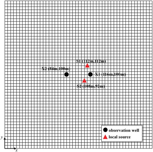
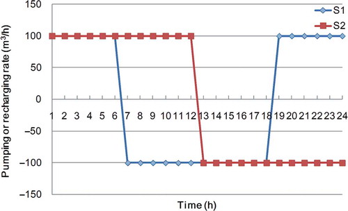
Two pumping and recharging wells, denoted by S1 and S2, are located near the middle of the site with the spatial coordinates (112 m, 112 m) and (108 m, 92m), respectively. The pumping and recharging rate is time variant, as shown in Fig. 3. For S1, the recharging starts at 01:00 h, ends at 06:00 h, restarts at 19:00 h and ends again at 24:00 h, with a constant rate of +100 m³/h. The pumping starts at 07:00 h and ends at 18:00 h, with a constant rate of –100 m³/h. For S2, the recharging starts at 01:00 h and ends at 12:00 h, with a constant rate of +100 m³/h. The pumping starts at 13:00 h and ends at 24:00 h, with a constant rate of –100 m³/h.

Fig. 3 Time series of pumping and recharging rate of two local sources.

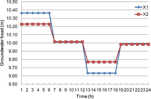
Two monitoring wells, denoted by X1 and X2, are located near the local source, with the spatial coordinates (116 m, 100 m) and (84 m, 100 m), respectively. The observation data are illustrated in Fig. 4. The head at monitoring well X1 varies from 10.37 to 9.63 m, while the head at monitoring well X2 varies from 10.23 to 9.77 m. The head fluctuation is higher at X1 because it is located near two local sources. Besides, the observed head fluctuation can be divided into four time periods: 1–6, 7–12, 13–18, and 19–24 h. During each time period, the groundwater head has its special pattern related to its pumping and recharging characteristics. But the observation data give a mixed signal, which is simultaneously influenced by two local sources. Through only the observed time series, it is hard to evaluate the extent to which one source has affected one observation. This is why the local source identification problem is hard to solve with limited observations. In the traditional source identification process, the source location and quantity are assumed to be unknown and only the simulation and optimization model without ICA is used to estimate local sources, i.e. 48 observations are used to estimate 52 unknowns (four for source location and 48 for the pumping and recharging time series). As a natural consequence of such an ill-posed problem, the estimation results diverge seriously. This is why we employ ICA in this paper to extract beforehand the characteristic pattern from the groundwater head observation data.

Fig. 4 Hourly groundwater head observation data obtained from two monitoring wells.

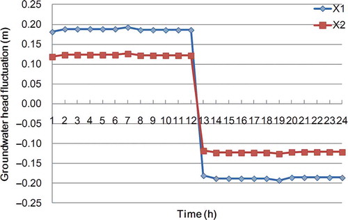
For ICA, the observation head at monitoring well X1 and X2 is the mixed signal X, while the head at local sources S1 and S2 is the original signal S, which is to be evaluated together with mixing matrix A. Each element in the AS matrix represents an independent head fluctuation caused by one single source, i.e. a_ij × s_j is the groundwater head fluctuation at monitoring well i caused by local source j. The head fluctuation at monitoring well X1 and X2 caused by local source S1 is shown in Fig. 5, and the corresponding head fluctuation caused by local source S2 in Fig. 6. It can be seen from Fig. 5 that the head fluctuation is the same as the pumping and recharging pattern of S1 shown in Fig. 3. In the same way the head fluctuation shown in Fig. 6 is the same as pumping and recharging pattern of S2. This explains why we referred to the groundwater head fluctuation extracted by ICA as the characteristic pattern. The most important characteristics are type and distance, where type means the type of pumping or recharging behaviour in one day, and pumpage for each different usage has a different type. For example, domestic water usage is highest just before and after working hours. In contrast, agricultural water usage is highest during working hours. The characteristic pattern has exactly the same type of water usage. In addition to the type of local source, the characteristic pattern also reveals the distance between source and observation. Take Fig. 6, for example: the magnitude of head fluctuation at X1 is always larger than that at X2. This clearly indicates that local source S2 is located near monitoring well X1 and far from X2. In summary, the shape of the characteristic pattern displays the pumping and recharging type of the local source; meanwhile, the amplitude of the characteristic pattern presents the distance between source and observation. These are the reasons that we claim that characteristic patterns extracted by ICA provide novel information on local pumping and recharging source identification and quantity estimation of a groundwater system.

Fig. 5 Groundwater head fluctuation at monitoring well X1 and X2 caused by local source S1.

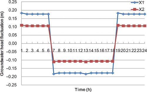
Fig. 6 Groundwater head fluctuation at monitoring well X1 and X2 caused by local source S2.

Moreover, the ill-posed problem is solved automatically after applying ICA. The original 48 counts of observation data, i.e. hourly observation data within 24 h from two observation wells, are separated independently into 96 observations. Of these, 48 observations relate to only one single local source S1, while the other 48 observations relate only to the other local source S2. The groundwater head fluctuation at monitoring wells X1 and X2 caused by local source S1 is chosen as observations to estimate local source S1; the groundwater head fluctuation at monitoring wells X1 and X2 caused by local source S2 is chosen as observations to estimate local source S2. Both single source identification problems are well-posed problems, since 48 observations are used to estimate 26 unknowns (two for source location and 24 for the pumping and recharging time series). ICA creates an ideal situation that only one source is pumping or recharging while all the monitoring wells are observing. Such an ideal situation is hard to meet in the field, but now is easily created by ICA. The numerous local sources could be properly identified one by one under sufficient observations.

3.1 Sensitivity analysis

Before applying the new observation data extracted from ICA in source identification, sensitivity analysis is carried out to assess if the new observation data are sensitive to the unknowns. The difference in objective function calculated with different guesses of unknowns should be significant enough to distinguish one suspected source from another. The sensitivity of observation with respect to unknown source location and quantity is calculated by the perturbation method. In practice, the sensitivity is equal to the objective function with the value of one chosen unknown increasing by one unit. For example, the true x coordinate of local source S1 is 112 m; the perturbed x coordinate can be 116 m (=112 m + discretized grid size); the sensitivity or objective function with the perturbed x coordinate is 1.29 × 10⁻³ m²/m. Similarly, the true recharging quantity at 04:00 h of the local source S1 is +100 m³; the perturbed recharging quantity can be +101 m³; the sensitivity calculated is 2.15 × 10⁻⁶ m²/m³, and so on. All the sensitivities of unknown source location and quantity at different times are listed in Table 1. Since all the sensitivities are greater than zero, it can be concluded that each observation setting is sensitive to the location and the quantity of local sources S1 and S2. Furthermore, the observation is more sensitive to the location than to the quantity. This may suggest that the source location is easier to identify than the pumping or recharging quantity. The sensitivity analysis of local source S2 is similar to that of S1. In other words, the new observation data extracted from ICA are capable of source identification.

Table 1 Sensitivities of unknown source location and quantity of local source S1 and S2.

Unknown	Sensitivity
	S1	S2
x coordinate	0.00128700 m^2/m	0.00606300 m^2/m
y coordinate	0.00613500 m^2/m	0.00488000 m^2/m
Pumping or recharging quantity in each hour	0.00000215 m^2/m^3	0.00000248 m^2/m^3

Here, we want to emphasize again the view, mentioned in Section 2.1, that the hourly groundwater head observations contain the most valuable information about characteristic pattern. This can be found in Fig. 4: if we take daily head as the observation, it is a constant head of 10 m. So, daily head contains no information about local source identification in the case study. This is a common situation, which one may encounter in the field. Because local source affects the groundwater system in finite space and time, any observation with a long time scale would smooth the information and detail of a short time scale. This is why hourly head observation is required and the results shown in Figs 5 and 6 clarify this viewpoint. The next step is to put the characteristic pattern into the groundwater simulation and optimization model as the new observation data to best estimate one local source location and quantity at a time.

3.2 Source identification

First, the groundwater head fluctuation at monitoring wells X1 and X2 caused by local source S1 is chosen as the observation and is put into the simulation and optimization model to identify the local source S1. That is, the characteristic pattern is given as new observation data at monitoring wells X1 and X2, and the groundwater simulation and optimization model is utilized to simulate the head variation and to optimize the source location and pumping or recharging rate. The optimization model quickly finds the exact solution in only 136 search times. Location, as well as the pumping and recharging time series of local source S1, are correctly identified as the real ones.

Secondly, the characteristic pattern of S2, as illustrated in Fig. 6, is used to identify local source S2. Again, the proposed source identification process combining ICA and optimization model follows a rational line, and is successful in the identification of S2 in 112 search times. This case study shows the correctness and efficiency of the proposed source identification process.

The results indicate that the ill-posed source identification problem is converted into several independent well-posed ones by adding novel information, called a characteristic pattern, obtained from ICA. The groundwater head fluctuation at monitoring wells induced by many local sources is a mixed signal. With the help of ICA, the fluctuation is separated into several small components. Each component represents the fluctuation caused by a single source. In other words, one local source is monitored by more than one monitoring well. If there are two monitoring wells, two local pumping or recharging sources can be identified; if there are three monitoring wells, three local pumping or recharging sources can be identified, and so on. As a result, the maximum number of local sources that can be identified is the same as the number of monitoring wells, as long as all the sources have a different characteristic pattern. This condition is easy to satisfy in reality, since it is very hard to find two sources with exactly the same characteristic pattern.

3.3 Robust analysis

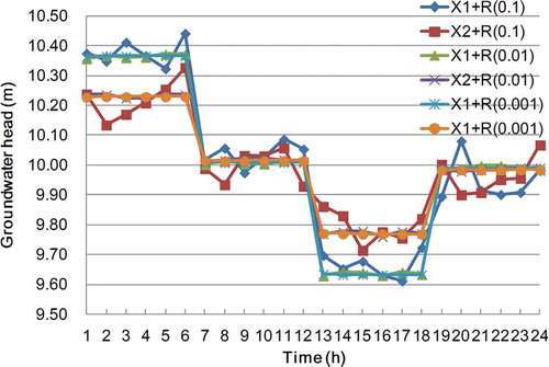
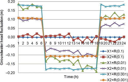
In real situations, some observation error may be embedded in observation data. The error can come from measuring instruments, human operation, or just random process. The success of the proposed methodology depends on whether ICA can independently and correctly identify the characteristic pattern of each source. From original observation data, ICA should be able to separate the groundwater head fluctuation caused by any single source. Robust analysis is required to test if ICA will work within an acceptable range of observation error. Three different magnitudes of random observation error, 0.1, 0.01 and 0.001 m, are added into the observation data to form three sets of observations, as shown in Fig. 7. The observation data with random error of 0.001 m are very close to the field situation, since most groundwater level meters are of centimetre or even millimetre precision. For the observation data with a random error of 0.1 m, the error is so large that this observation set cannot offer meaningful information on source identification.

Fig. 7 Observation data with different magnitude of random observation error.

After the source identification process, three observation sets are first separated by ICA to obtain the groundwater head fluctuation, i.e. characteristic pattern, at monitoring wells caused by local sources S1 and S2, as illustrated in Figs 8 and 9, respectively. It can be seen from both Figs 8 and 9 that the characteristic pattern is clearly identified with an observation error of 0.001 m. As the error increases, the extracted result gets worse. The characteristic pattern extracted from observation with random error of 0.01 m can still display the pumping and recharging trend of the local source, but the detail is a little disturbed. When the observation error reaches a magnitude of 0.1 m, the extracted pattern has nothing in common with the character of the local source and is almost the same as observation. These phenomena indicate that ICA has the ability to recognize the character of a local source under a reasonable range of observation error. Nevertheless, ICA still has its limitations: it does not work when no information can be extracted from the original signals. That is the situation encountered in the case of 0.1 m observation error. The results of source identification also support the findings.

Fig. 8 Characteristic pattern of local source S1 extracted by ICA with different magnitude of random observation error.

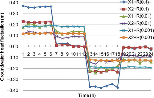
Fig. 9 Characteristic pattern of local source S2 extracted by ICA with different magnitude of random observation error.

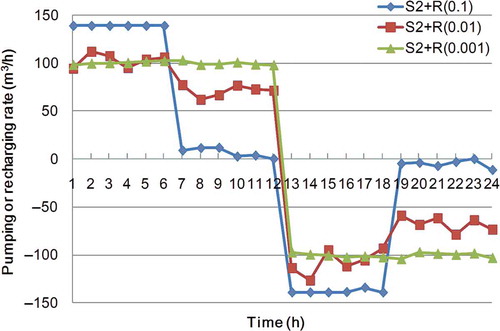
Three different sets of characteristic pattern are used for source identification to estimate the source location and quantity. The two with a small observation error are able to identify the source location, i.e. (116 m, 100 m) and (84 m, 100 m), while the one with a large observation error fails to locate the source, as expected. The identified pumping and recharging time series of local sources S1 and S2, with a different magnitude of random observation error, are plotted in Figs 10 and 11, respectively. Through the proposed source identification process, not only the location but also the quantity of two local sources is correctly identified as long as the observation error is of reasonable magnitude. As illustrated in Figs 10 and 11, observation with an error of 0.001 m is acceptable. The identified quantity is almost the same as the true one, with a difference of 4 m³/h at most. Even when the observation error becomes as large as 0.01 m, the identification process still can catch the basic trends of pumping and recharging. Besides, the difference between the true solution and the identified one converges in a small range within 40 m³/h. The results show the robustness and practicability of the proposed source identification process. Importing ICA into the groundwater simulation and optimization model stabilizes the source identification problem and also brings out novel information on local sources. Thus the proposed methodology enables further research on source identification.

Fig. 10 Identified pumping and recharging time series of local source S1 with different magnitude of random observation error.

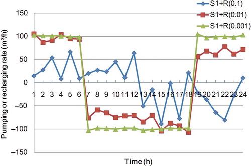
Fig. 11 Identified pumping and recharging time series of local source S2 with different magnitude of random observation error.

4 CONCLUSIONS

In this paper, a series of research papers concerning source identification, as well as pumping or recharging rate estimation have been reviewed. This indicates that local sources are difficult to identify because of limited information. The groundwater head observation obtained at monitoring wells is the most informative data, but all the observations are mixed signals and indirect measures of local source. Lack of sufficient information limited the development of source identification.

The statistical technique, independent component analysis, is introduced to evaluate the head fluctuation at every monitoring well caused by a single local source. That is, through ICA, we create a situation that only one well is pumping or recharging, while all monitoring wells are observing. Such a situation can never happen in the field. But, through the ability of source separation and feature extraction in ICA, such a situation can be realized. The number of observations does not increase, but the information about unknown sources increases. Therefore, the ill-posed source identification problem is now converted into several independent well-posed ones and is easy to solve.

Moreover, the decomposed head fluctuation at a monitoring well caused by a local source contains meaningful information and is specially named the ‘characteristic pattern’. The shape of the characteristic pattern displays the pumping and recharging type of the local source; meanwhile, the amplitude of the characteristic pattern presents the distance between source and observation. Characteristic patterns extracted by ICA provide novel information on local sources. Thus, local pumping and recharging source identification and quantity estimation of groundwater can be correctly solved by combining ICA with a groundwater simulation and optimization model.

A hypothetical case clearly shows the accuracy and efficiency of the proposed source identification process. Without ICA, the number of observations is less than that of unknowns and the solution is divergent. Through ICA, the characteristic patterns are extracted and reveal the characters of local pumping and recharging. Through adding novel information and decreasing the number of unknowns, the source identification problem can be solved correctly and efficiently. The maximum number of local sources that could be identified is extended to the number of monitoring wells, as long as the characteristic pattern of any two of the local sources is not the same. This is a basic restriction of ICA, but it may not cause any problem in its application to groundwater modelling, since the pumping behaviour of different sources varies in a local region. Moreover, the novel information can be widely used for source identification and provides a new vision for groundwater resources management. The pumping and recharging behaviour of local sources can be further discussed for an hourly time scale.

The proposed method is basically successful in the case of source identification in a confined aquifer. When applied to an unconfined aquifer, it may suffer a strong nonlinear effect of the observed head response to pumping or recharging. Besides, the head variation in an unconfined aquifer is less than that in a confined aquifer. The limitations of the proposed method can be further tested. Furthermore, in large-scale (such as groundwater basin) application, there are thousands of pumping wells together with dozens of observation wells. Thus observation may be very limited, so it is impossible to identify every single pumping well. However, with some adjustment, the method provided herein can still work in reality. The adjustment is to give up the idea of identifying one pumping well; instead, it is to identify one pumping behaviour of a specific kind of water usage, i.e. agricultural, industrial, or domestic pumpage. Such adjustment has to be further tested and more research needs to be done.

Finally, we want to stress the importance of observation frequency. The commonly used sampling frequency for a monitoring network in the field is once a day. Daily observation is therefore applied in groundwater modelling for many applications. However, daily observation does not seem to work well for local source identification. This is because the pumping and recharging of a local source is dominated by human activities. People act hour by hour not all day long, which leads to an hourly variation pattern of the local source. Consequently, hourly groundwater head observation data are most suitable and required for local source identification.

Last, but most important of all, we bring up a whole new idea about source identification: the success of unknown estimation depends on the information not the observations one can gain. In reality, the observation data are limited. The number of unknowns is often larger than that of observations, so we should try to extract as much information as possible from observations instead of trying to increase the number of observations. One may extract different kinds of information by applying different kinds of data analysis techniques. Some information, such as the characteristic pattern extracted by ICA, can be very useful in helping us to understand the real world.

Disclosure statement

No potential conflict of interest was reported by the authors.

Acknowledgements

We gratefully acknowledge the Civil and Environmental Engineering Department, University of California, Los Angeles, Prof. William W.-G. Yeh for his participation in the discussion and providing academic advice.

Additional information

Funding

We would like to express our gratitude for the financial support granted by the Water Resources Agency, Ministry of Economic Affairs, Taiwan (Project no. MOEAWRA0990409).

REFERENCES

- AnCAD Inc., 2011. Visual signal reference guide, version 1.4. Taipei: AnCAD Inc. Available from: http://www.ancad.com.tw/VS_Online_Help_1.4/index1.html?page=ar01.html
- Aral, M.M., Guan, J., and Maslia, M.L., 2001. Identification of contaminant source location and release history in aquifers. Journal of Hydrologic Engineering, 6, 225–234. 10.1061/(ASCE)1084-0699(2001)6:3(225).
- Ayvaz, M.T. and Karahan, H., 2008. A simulation/optimization model for the identification of unknown groundwater well locations and pumping rates. Journal of Hydrology, 357, 76–92. doi: 10.1016/j.jhydrol.2008.05.003.
- Calderhead, A.I., et al., 2012. Sustainable management for minimizing land subsidence of an over-pumped volcanic aquifer system: tools for policy design. Water Resources Management, 26, 1847–1864. doi:10.1007/s11269-012-9990-7.
- Cheng, W.-C., et al., 2009. A nudging data assimilation algorithm for the identification of groundwater pumping. Water Resources Research, 45, W08434. doi:10.1029/2008WR007602.
- Chiu, Y.C., et al., 2009. Development of an objective-oriented groundwater model for conjunctive-use planning of surface water and groundwater. Water Resources Research, 45, W00B17. doi:10.1029/2007WR006662.
- Chou, P.Y. and Ting, C.S., 2007. Feasible groundwater allocation scenarios for land subsidence area of Pingtung Plain, Taiwan. Water Resources, 34, 259–267. doi:10.1134/S0097807807030037.
- Don, N.C., et al., 2005. Simulation of groundwater flow and environmental effects resulting from pumping. Environmental Geology, 47, 361–374. doi:10.1007/s00254-004-1158-1.
- Galloway, D.L. and Burbey, T.J., 2011. Review: regional land subsidence accompanying groundwater extraction. Hydrogeology Journal, 19, 1459–1486. doi:10.1007/s10040-011-0775-5.
- Groisman, P.Y., et al., 2005. Trends in intense precipitation in the climate record. Journal of Climate, 18, 1326–1350. doi:10.1175/JCLI3339.1.
- Hyvärinen, A., 1998. Independent component analysis in the presence of Gaussian noise by maximizing joint likelihood. Neurocomputing, 22, 49–67. doi:10.1016/S0925-2312(98)00049-6.
- Hyvärinen, A., 1999a. Fast and robust fixed-point algorithms for independent component analysis. IEEE Transactions on Neural Networks, 10, 626–634. doi:10.1109/72.761722.
- Hyvärinen, A., 1999b. Survey on independent component analysis. Neural Computing Surveys, 2, 94–128.
- Hyvärinen, A. and Oja, E., 1997. A fast fixed-point algorithm for independent component analysis. Neural Computation, 9, 1483–1492.
- Hyvärinen, A. and Oja, E., 2000. Independent component analysis: algorithms and applications. Neural Networks, 13, 411–430. doi:10.1016/S0893-6080(00)00026-5.
- Jutten, C. and Herault, J., 1991. Blind separation of sources, part I: an adaptive algorithm based on neuromimetic architecture. Signal Processing, 24, 1–10. doi:10.1016/0165-1684(91)90079-X.
- Koutsoyiannis, D., 2011. Scale of water resources development and sustainability: small is beautiful, large is great. Hydrological Sciences Journal, 56 (4), 553–575. doi:10.1080/02626667.2011.579076.
- Lee, J.Y., et al., 2005. Evaluation of hydrologic data obtained from a local groundwater monitoring network in a metropolitan city, Korea. Hydrological Processes, 19, 2525–2537. doi:10.1002/hyp.5689.
- Lin, Y.C. and Yeh, H.D., 2008. Identifying groundwater pumping source information using simulated annealing. Hydrological Processes, 22, 3010–3019. doi:10.1002/hyp.6875.
- Liu, H.-J., Hsu, N.-S., and Lee, T.-H., 2009. Simultaneous identification of parameter, initial condition, and boundary condition in groundwater modelling. Hydrological Processes, 23, 2358–2367. doi:10.1002/hyp.7344.
- Llamas, R., 2004. Water and ethics: use of groundwater. Paris: UNESCO. ISBN 92-9220-022-4.
- Mahinthakumar, G. and Sayeed, M., 2005. Hybrid genetic algorithm-local search methods for solving groundwater source identification inverse problem. Journal of Water Resources Planning and Management-ASCE, 131, 45–57.
- Misstear, B.D.R., Brown, L., and Johnston, P.M., 2009. Estimation of groundwater recharge in a major sand and gravel aquifer in Ireland using multiple approaches. Hydrogeology Journal, 17, 693–706. doi:10.1007/s10040-008-0376-0.
- Nelson, R.L., 2012. Assessing local planning to control groundwater depletion: California as a microcosm of global issues. Water Resources Research, 48, W01502. doi:10.1029/2011WR010927.
- Peng, T.R., et al., 2010. Identification of groundwater sources of a local-scale creep slope: using environmental stable isotopes as tracers. Journal of Hydrology, 381, 151–157. doi:10.1016/j.jhydrol.2009.11.037.
- Porter, D.W., et al., 2000. Data fusion modeling for groundwater systems. Journal of Contaminant Hydrology, 42, 303–335. doi:10.1016/S0169-7722(99)00081-9.
- Rao, S.V.N., 2006. A computationally efficient technique for source identification problems in three-dimensional aquifer systems using neural networks and simulated annealing. Environmental Forensics, 7, 233–240. doi:10.1080/15275920600840560.
- Ruud, N., Harter, T., and Naugle, A., 2004. Estimation of groundwater pumping as closure to the water balance of a semi-arid, irrigated agricultural basin. Journal of Hydrology, 297, 51–73. doi:10.1016/j.jhydrol.2004.04.014.
- Safavi, H.R., Darzi, F., and Mariño, M.A., 2010. Simulation-optimization modeling of conjunctive use of surface water and groundwater. Water Resources Management, 24, 1965–1988. doi:10.1007/s11269-009-9533-z.
- Saffi, M. and Cheddadi, A., 2007. Explicit algebraic influence coefficients: a one-dimensional transient aquifer model. Hydrological Sciences Journal, 52, 763–776. doi:10.1623/hysj.52.4.763.
- Saffi, M. and Cheddadi, A., 2010. Identification of illegal groundwater pumping in semiconfined aquifers. Hydrological Sciences Journal, 55 (8), 1348–1356. doi:10.1080/02626667.2010.520560.
- Sun, N.-Z., 2005. Structure reduction and robust experimental design for distributed parameter identification. Inverse Problems, 21, 739–758. doi:10.1088/0266-5611/21/2/018.
- Teatini, P., et al., 2006. Groundwater pumping and land subsidence in the Emilia-Romagna coastland, Italy: modeling the past occurrence and the future trend. Water Resources Research, 42, W01406. doi:10.1029/2005WR004242.
- Tung, C.P. and Chou, C.A., 2004. Pattern classification using tabu search to identify the spatial distribution of groundwater pumping. Hydrogeology Journal, 12, 488–496. doi:10.1007/s10040-004-0344-2
- Wang, C.-H., et al., 2005. Some isotopic and hydrological changes associated with the 1999 Chi-Chi earthquake, Taiwan. The Island Arc, 14, 37–54. doi:10.1111/j.1440-1738.2004.00456.x.
- Wittenberg, H. and Sivapalan, M., 1999. Watershed groundwater balance estimation using streamflow recession analysis and baseflow separation. Journal of Hydrology, 219, 20–33. doi:10.1016/S0022-1694(99)00040-2.