A new fuzzy linear regression approach for dissolved oxygen prediction

Abstract

A new method for fuzzy linear regression is proposed to predict dissolved oxygen using abiotic factors in a riverine environment, in Calgary, Canada. The proposed method is designed to accommodate fuzzy regressors, regressand and coefficients, i.e. representing full system uncertainty. The regression equation is built to minimize the distance between fuzzy numbers, and generalizes to crisp regression when crisp parameters are used. The method is compared to two existing fuzzy linear regression techniques: the Tanaka method and the Diamond method. The proposed new method outperforms the existing methods with higher Nash-Sutcliffe efficiency, and lower RMSE, AIC and total fuzzy distance. The new method demonstrates that nonlinear membership functions are more suitable for representing uncertain environmental data than the typical triangular representations. A result of this research is that low DO prediction is improved and consequently the approach can be used for risk analysis by water resource managers.

Editor D. Koutsoyiannis; Associate editor T. Okruszko

Une nouvelle approche de régression linéaire floue pour la prévision de l’oxygène dissous

Résumé Nous proposons une nouvelle méthode de régression linéaire floue afin de prévoir l’oxygène dissous en utilisant des facteurs abiotiques d’un environnement fluvial, à Calgary, au Canada. La méthode proposée est conçue pour intégrer des variables explicatives floues, une variable dépendante et des coefficients, représentant ainsi l’incertitude totale du système. L’équation de régression est conçue pour minimiser la distance entre nombres flous, et se généralise à la régression bornée lorsque des paramètres bornés sont utilisés. La méthode est comparée à deux techniques existantes de régression linéaire floue: la méthode Tanaka et la méthode Diamond. La méthode proposée fait mieux que les méthodes existantes avec un meilleur coefficient de Nash-Sutcliffe et avec une racine de l’écart quadratique moyen, un critère d’information d’Akaike (CIA) et une distance floue totale plus petits. La nouvelle méthode montre que l’utilisation de fonctions d’appartenance non-linéaires est plus appropriée pour représenter des données environnementales incertaines par rapport aux représentations triangulaires typiques. Un résultat de cette recherche est que la prévision des faibles valeurs d’oxygène dissous est améliorée, et que l’approche peut être utilisée pour l’analyse de risques par les gestionnaires des ressources en eau.

Key words:

• dissolved oxygen
• fuzzy numbers
• linear regression
• fuzzy linear regression
• uncertainty
• risk
• water quality

Mots clefs:

• oxygène dissous
• nombres flous
• régression linéaire
• régression linéaire floue
• incertitude
• risques
• qualité de l’eau

1 INTRODUCTION

Dissolved oxygen (DO) is an important water quality parameter and is often used as an indicator of overall aquatic ecosystem health. DO concentration in water bodies influences biotic communities and is vital for their survival (He et al. 2011). For these reasons, DO is a parameter of concern and is routinely monitored by water resource managers. A number of factors can cause low DO, thereby increasing the risk of adverse effects on the aquatic environment. Both biotic and abiotic (non-living, physical and chemical attributes) factors influence DO concentration in riverine environments. These affects can be direct or indirect. For example, macrophyte growth can directly cause variation in DO concentration through photosynthesis and respiration (Pogue and Anderson 1995, Hauer and Hill 2007). In contrast, discharge rate influences macrophyte population, which in turn affects DO concentration.

The physical processes that govern the behaviour of DO in the aquatic environment are quite complex and poorly understood. Furthermore, modelling DO behaviour requires the parameterization of a large number of variables (Khan et al. 2013). Thus, predicting DO concentration in riverine environments is not only challenging, but is filled with uncertainty that is generally unknown. This increases the difficulty in decision making for water resource managers and also increases the risks to aquatic ecosystems. Thus, a method is needed that can accurately predict DO concentration that is not limited by the lack of understanding of governing processes and at the same time, circumvents the parameterization issues and data hurdles that plague modelling. In addition, the method must capture the uncertainty and variability in DO prediction so that complete and useful information can be provided to managers. In this research, a new method to predict DO concentration that satisfies these two requirements is proposed. It uses a combination of abiotic factors, data-driven techniques and fuzzy set theory.

1.1 Background

In a highly urbanized reach of the Bow River, in Calgary, Alberta, Canada, occasional low DO concentrations have been observed. A number of abiotic factors (influenced by urbanization) seem to affect DO concentration and variability at sites downstream of the effluent discharge from a wastewater treatment plant (He et al. 2011, Khan et al. (2013). The City of Calgary is mandated to maintain DO concentration above the Alberta provincial guideline of 5 mg/L (one day minimum limit) (Alberta Environment Protection 1997). Thus, monitoring and modelling DO concentration is part of the compliance program of the City of Calgary. Recent studies by He et al. (2011) and Khan et al. 2013) have used data-driven modelling techniques (e.g. multiple linear regression and multiple layer perceptron neural networks) with abiotic factors to predict DO concentration in the Bow River in the absence of both sufficient biotic data, and knowledge of the physical processes underlying DO trends in the river. In these studies, abiotic factors such as water temperature, river discharge, solar radiation, and pH, were analyzed to see if they can be used to predict daily DO concentration and variability. The rationale of identifying which abiotic factors, and to what extent they influence DO concentration, is that if the former can be controlled, the latter can be indirectly improved. The results from these studies show that a data-driven approach is appropriate to predict DO concentration in the Bow River.

Another implication of the success of these studies is that the developed models can be used to predict when (and possibly where) low DO concentration may occur in the Bow River. This extends the application of these models from simple predictions to risk assessment. For example, if forecast data suggest that the abiotic factors are expected to be such that the data-driven models predict potentially low DO concentration, a probability and risk of ‘DO being below 5 mg/L’ can be assigned. However, data-driven modelling has intrinsic uncertainties associated with it. This uncertainty must be identified and propagated through the model before important decisions based on the output can be made (Shrestha and Nestmann 2009). Scarcity, measurement errors, randomness and scaling issues are a few examples of the different sources of uncertainty, each of which can affect model projections (Zhang et al. 2009). In addition, uncertainty may also increase when data from numerous sources are used, integrated and propagated (Porter et al. 2000, Shrestha and Nestmann 2009, Hermann 2011). Fuzzy numbers and its extension, possibility theory, are one approach for dealing with these types of uncertainty.

1.2 Uncertainty analysis using fuzzy numbers

Fuzzy set theory was first proposed by Zadeh (1965) and can be described as a generalization of classical set theory. In classical set theory, an element x  either belongs or does not belong to a set A. In contrast, using fuzzy set theory, the elements x of a fuzzy set à have a degree of membership within that set. This degree of membership is defined as a value between 0 and 1. Here a membership level, µ, equal to 0 means that x does not belong in Ã, a value µ = 1 means that it completely belongs in set Ã, while a value µ = 0.5 means that it is only a partial member of Ã. By these definitions, a traditional set (known as a crisp set to distinguish it from a fuzzy set) is a special case of a fuzzy set: when x is a member of A, its membership level µ is equal to 1, and when x does not belong to A, µ = 0. The collection of membership levels that define a fuzzy number is known as its membership function. Fuzzy sets have recently been used in a variety of hydrological and environmental applications (Wang and Huang 2012, Han et al. 2013, Wang and Huang 2013a, 2013b).

Fuzzy set theory was developed to describe uncertain or imprecise information. A fuzzy number is an extension of fuzzy set theory, and expresses an uncertain or imprecise quantity. In much the same way that a fuzzy set generalizes a crisp set, a fuzzy number generalizes a real number. A fuzzy number does not refer to a single value, but represents the set of all possible values that define it. The nature of fuzzy numbers lends itself well to uncertainty analysis and is one technique for characterizing and aggregating uncertain data (Khan et al. 2013). It is particularly useful for dealing with uncertainties when data are limited or imprecise (Bárdossy et al. 1990, Guyonnet et al. 2003, Huang et al. 2010, Zhang and Achari 2010a). In these cases, a probabilistic representation of parameters may not be possible, since the exact values of parameters may be unknown, or only partial information is available (Zhang 2009). In such a situation, fuzzy techniques can be used to transform uncertainty from traditional probabilistic to ‘possibilistic’ representation (Xia et al. 2000).

Fuzzy numbers, along with possibility theory (the extension of probability theory for fuzzy numbers), has been widely used in hydrology to represent uncertainty in the parameters of numerical models. A popular application has been to represent water level and discharge rate as fuzzy numbers to improve stage–discharge relationships (Alvisi et al. 2006, Shrestha et al. 2007, Alvisi and Franchini 2011). Another approach has been to model the contaminant transport phenomenon using fuzzy numbers to represent uncertainty in groundwater systems, including contaminant concentration and subsurface characteristics (Dou et al. 1997, Freissinet et al. 1999, Abebe et al. 2000, Kumar et al. 2006, Zhang et al. 2009). Fuzzy number-based methods have also been developed to link contaminant concentration to health risk assessment in groundwater systems (Chen et al. 2003, Guan and Aral 2004, Kentel and Aral 2004, Kumar et al. 2006). In a different type of application, Maskey et al. (2004) used fuzzy numbers to describe a rainfall–runoff process, where the temporal uncertainty in precipitation was represented by fuzzy numbers. Another example, an early application in hydrology, was illustrated by Bárdossy et al. (1990), who used fuzzy numbers to study an imprecise relationship between soil electrical resistivity and hydraulic permeability. In more recent studies, fuzzy set theory has been used in water resource management problems, where uncertainties from multiple sources and types have been combined.

Applications involving DO have also been developed, though they do not specifically use fuzzy numbers, but use other fuzzy set theory-based methods, such as fuzzy logic and fuzzy pattern recognition. Mujumdar and Sasikumar (2002) defined the risk of the occurrence of low DO concentration as a fuzzy event, i.e. instead of assigning one value to the probability of a low DO event, a range of values in the form of a fuzzy set are defined. Giusti and Marsili-Libelli (2009) used a fuzzy pattern recognition technique to define the natural variation, and to predict the dynamics of DO in a lagoon. Altunkaynak et al. (2005) also modelled DO dynamics, and used a fuzzy logic inference system for forecasting using artificial neural networks.

The literature clearly demonstrates the utility and advantage of using fuzzy numbers in environmental problems. In the examples discussed above, the representation of uncertain data (e.g. hydraulic conductivity or contaminant concentration) as fuzzy numbers has been widely used, although the techniques have varied. However, the representation of fuzzy relationships or systems has been limited. In the case of the Bow River in Calgary, uncertainty exists not only in the abiotic parameters used to predict DO concentration, but also in the relationships between the abiotic factors and DO. Thus, a method that uses fuzzy numbers to represent parameter and system uncertainty to predict DO concentration using a data-driven approach would be highly advantageous to water resource managers. Mathematical techniques have been developed, each suited to the particular application, to use fuzzy numbers in crisp relationships (e.g. in physically-based models). To correctly incorporate fuzzy numbers into numerical models, be it physically-based or data-driven, classical mathematics needs to be adapted to account for fuzzy numbers. Fuzzy arithmetic (covered in detail in Kaufmann and Gupta 1984, and also briefly described in the Appendix), including the extension principle and the α-cut approach, has been developed to provide these tools.

1.3 Fuzzy linear regression

Linear regression is a widely-used data-driven technique for prediction. The general purpose of regression is to explain the uncertainty and variability in a dependent variable through a series of explanatory or independent variables, leading to a prediction equation (Bárdossy 1990, Bárdossy et al. 1990, Peters 1994, Chang and Ayyub 2001, Kahraman et al. 2006). When large datasets are available, regression may provide realistic results, but in its absence, as is often the case in hydrological applications, statistical regression should not be used (Bárdossy et al. 1990). Furthermore, statistical regression is inappropriate when it is difficult to verify strict distribution assumptions (including whether or not the data are mutually independent and identically distributed), and vagueness and ambiguity exists in the relationships between variables (Peters 1994, Kim et al. 1996, Kahraman et al. 2006). Fuzzy linear regression is an attempt to extend linear regression for applications involving fuzzy numbers. It provides an alternative method in situations where crisp linear regression may not be possible, whether it be due to the inability to meet strict assumptions, or if there is obvious fuzziness in the underlying data or process (Bárdossy et al. 1990, Kim et al. 1996, Kahraman et al. 2006). A number of different fuzzy linear regression methods have been created, each aiming to mimic the concept of crisp regression but with fuzzy numbers.

In crisp regression, deviations from the true data can be caused by measurement and modelling error. Though measurement error may be well defined, modelling error (which would occur even if using precise data) is often not (Bárdossy 1990, Chang and Ayyub 2001). However, fuzzy regression tries to capture the vagueness, and the non-random or fuzzy error in the model structure: it is assumed that deviations are due to system fuzziness, i.e. the fuzziness of the regression coefficients. These two distinct types of uncertainty are only part of the overall uncertainty. Ordinary linear regression provides tools that are suitable for dealing with crisp data, but only when the true relationships between the data are known (Peters 1994, Chang and Ayyub 2001, Lee and Chen 2001, Kahraman et al. 2006).

There are two major types of fuzzy regression. The first is known as ‘possibilistic’ fuzzy regression, developed by Tanaka et al. (1982), which is a linear programming approach that aims to minimize the fuzziness of the system. The second is a fuzzy least-squares approach, where, in broad terms, the distance between two fuzzy numbers is minimized (Diamond 1988, Kahraman et al. 2006). The goal of each method is to fit fuzzy data within a specific fitting criterion. The choice of criterion, whether it is to minimize system fuzziness or to minimize the distance between fuzzy numbers, governs the final regression equation (Chang and Ayyub 2001). In addition, there is a choice in the type of parameters to be used: fuzzy or crisp input data, fuzzy or crisp output data, and fuzzy or crisp regression coefficients (i.e. fuzzy relationships). This type of flexibility allows fuzzy regression to provide application-specific formulations.

The advantage of using fuzzy regression is that some of the strict assumptions of the statistical model can be relaxed (Bárdossy et al.1990, Peters 1994). In classical regression it is assumed that each error in the predicted variable is the same, whereas in fuzzy regression, the individual membership function describes the unique uncertainty of the variable. In addition, fuzzy regression can provide an insight into physical systems even with small sets of data; in fact, the performance of fuzzy regression models improves (as compared to crisp regression) when the size of the datasets is reduced (Bárdossy et al. 1990, Kim et al. 1996). Another benefit of fuzzy regression is that it can provide better generalization of data trends or patterns compared to crisp data (Bargiela et al. 2007). This is because the membership functions associated with fuzzy numbers have significant and useful information that is not incorporated in crisp regression.

1.3 Objectives

In this paper, the use of fuzzy numbers to characterize and propagate the uncertainty in a data-driven system for predicting daily DO concentration in a riverine environment is explored. Specifically, the objectives are: (a) to characterize the abiotic factors (limited to the discharge rate Q and water temperature T) that influence DO concentration as fuzzy numbers; and (b) to determine the efficacy of using fuzzy numbers to predict daily DO concentration and its uncertainty with a fuzzy linear regression model. To meet the first objective, an algorithm is described to convert a series of imprecise, highly variable and uncertain crisp measurements into fuzzy numbers. The second objective is accomplished through an improved fuzzy linear regression technique proposed to predict fuzzy daily DO concentration using fuzzy abiotic input parameters. The proposed new method is compared to two popular fuzzy linear regression techniques to highlight its novelty and significant results. The results from this method are then used to illustrate the benefit of using fuzzy numbers as opposed to crisp numbers. Data from the Bow River in Calgary are used to illustrate this methodology.

2 METHODOLOGY

2.1 Site description and data collection

The Bow River flows southeastwards from its headwaters in the Rocky Mountains through the foothills and the Prairies before reaching the City of Calgary. The average annual discharge in the Bow River within the city limits is approximately 90 m³/s and the average width and depth of the river are 100 m and 1.5 m, respectively. Three wastewater treatment plants (WWTP) located at Fish Creek, Bonnybrook and Pine Creek (Fig. 1) discharge their effluent into the Bow River.

Fig. 1 Aerial view of the City of Calgary, highlighting the Bow River, the Water Survey of Canada (WSC) monitoring station, and the Bonnybrook (BB), Fish Creek (FC) and Pine Creek (PC) wastewater treatment plants.

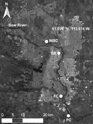
The objective of this study is to predict daily DO concentration using two abiotic factors, namely the discharge rate, Q, and river water temperature, T. The reasons for selecting these two parameters have been discussed previously in He et al. (2011) and Khan et al. (2013). The required data were collected from various sources. Hourly Q measurements from the Water Survey of Canada (WSC) were collected for the monitoring station ‘Bow River at Calgary 05BH005’ which is highlighted in Fig. 1 (Environment Canada Water Office 2013). Water quality data, specifically DO concentration and T, were measured using continuous YSI sondes from Pine Creek (PC in Fig. 1), which is approximately 20 km downstream of the Bonnybrook WWTP. The sondes were calibrated on a weekly basis and recorded water quality data every 15 min; though the interval increased to 30 min on some days.

Data for each variable were collected for the period 22 May–22 November for the years 2006, 2007 and 2008. This period coincides with the ice-free period in the Bow River, beyond which these data are typically not collected. During this period, the average annual Q ranged from 99.10 to 131.83 m³/s, while the minimum and maximum observed Q was 48.67 and 352.17 m³/s, respectively. Low flows are typically observed from January until the onset of spring freshet in May, when snowpack melt from the Rocky Mountains starts to contribute to flows. Discharge peaks in mid-June due to the combination of snowmelt from the mountains and precipitation within the watershed. The discharge then reduces until late October when baseflow conditions are reached (Alberta Environment River Basins 2012).

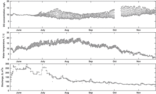
Average annual DO concentration ranged from 9.52 to 10.02 mg/L throughout the study period, while the minimum and maximum observed concentration was 3.81 and 18.32 mg/L, respectively. On an annual basis, the occurrence of low DO concentration tends to occur during the summer months, corresponding to low flows and high temperatures. This critical period corresponds to the selected research period. Typically, daily minimum DO concentration is high and daily DO variability is low during the winter, ice-covered period, when the risk to aquatic habitat is negligible. Note that DO concentrations fell below the provincial guidelines of 5 mg/L in 2006, but not in 2007 or 2008. The average annual T for the study period was in the range 11.72°C to 12.96°C, while the minimum and maximum were –0.05 and 22.44°C, respectively. None of the parameters exhibited a significant trend (p = 0.05) during the monitoring period. A sample time series plot of sub-daily observations for the three variables in 2008 is shown in Fig. 2.

Fig. 2 Daily observations of DO concentration, water temperature, T, and discharge, Q, in the Bow River for the ice-free period (May–November) in 2008. Note that DO and T data were collected every 15 min, while Q data were collected hourly.

2.2 Creating fuzzy numbers

The definition of a fuzzy set can be found in many textbooks on the subject (e.g. Kaufmann and Gupta 1984, DuBois and Prade 1980, Novák 1989). A fuzzy quantity is a numerical representation of imprecise data using fuzzy sets. A fuzzy number is a specific type of fuzzy quantity, one that aims to represent one particular quantity, rather than an interval of values. The mathematical definition of a fuzzy number is detailed in the Appendix, including that of a triangular (‘L-R’) fuzzy number, which is the most common and simplest realization of fuzzy numbers. These types of fuzzy numbers have membership functions defined by only three points (the lower and upper bound where µ = 0, and the modal value where µ = 1), and assume that the membership level monotonically increases, linearly from the lower bound to the modal value, and then monotonically decreases, linearly to the upper bound. These types of fuzzy numbers are believed to provide a reasonable representation of the possible values of a variable. Being linear functions, triangular fuzzy numbers are computationally inexpensive, but may not sufficiently describe the membership level of observed data. Other shapes for membership functions are also prevalent and may provide a more realistic representation of the observed data (Khan et al. 2013). By necessity, these nonlinear functions are defined at more than three membership levels (e.g. µ = 0.25, 0.50, 0.75 and so on), and are thus referred to as higher resolution membership functions.

The membership function of a fuzzy number is mathematically equivalent to its possibility distribution, and the terms are often used interchangeably (Zadeh 1978). However, it is important to note that possibility or degree of membership of a variable should not be confused with the probability or likelihood of occurrence. Possibility and probability are conceptually different: possibility theory is built on the weakness of probability theory, and does not subscribe to additivity (Zhang 2009). In probability theory, the probability of an event completely determines the probability of the contrary or complementary event (i.e. it is self-dual) (Dubois et al. 2004). However, in possibility theory the event and contrary event are only weakly linked (Dubois and Prade 1988). Since these are distinct concepts, it is possible to define the probability associated with some fuzzy number being measured (e.g. the probability that observed DO will be below the Alberta guideline), and the corresponding possibility distribution of the observed DO, given by its membership function (e.g. DÕ = {5.0, 4.8, 5.2} mg/L, using notation described in equation (A2)). Detailed discussion and a derivation of the possibility distribution can be found in Zadeh 1978) and Dubois and Prade (1988).

The Appendix details three concepts, α-cuts, the extension principle, and probability–possibility transformations, which are all used to convert crisp data to fuzzy numbers. Briefly, the α-cut technique provides a bridge to connect fuzzy sets to crisp sets (Zhang et al. 2009, Zhang and Achari 2010b, Wang et al. 2011, 2012). The extension principle (Zadeh 1975) provides a method for extending crisp mathematical functions to deal with fuzzy numbers. A probability–possibility transformation uses the α-cut and extension principle to transform crisp data to fuzzy numbers (Dubois et al. 1993, 2004, Zhang et al. 2009).

The data described in Section 2.1 were converted to a fuzzy number using a probability–possibility transformation detailed in the Appendix. The intention was to combine sub-daily measurements of a variable (e.g. Q, T or DO) into one fuzzy number representation of a daily measurement. Using this method, as opposed to the common approach of using mean daily data, all available information is contained in the fuzzy number. This fuzzy number not only characterizes the magnitude of the modal value of the daily observations, but also the variability, i.e. the support (the left and right bounds) and the probability of the data distribution, indirectly through the membership function. The specific algorithm developed to conduct this transformation for the T, Q and DO data is described below.

A daily data array, X, of length N, representing the N observations in a 24-h period, was collected for each variable. The first step is to calculate the probability density function (pdf) of the given array. The data were sorted into bins, and the number of observations in each bin was calculated. This series represented the pdf of the daily data. This pdf has to be created to ensure it is uni-modal, which means that it is a function of the bin size. Another constraint on the bin size is that it cannot be smaller than the sensitivity of the instrument used to measure each of the variables. This error term, ε, was subtracted from the minimum (X_min) and maximum (X_max) values of X, essentially to extend the support of the fuzzy number. The magnitude of ε is ±0.3°C for T; the greater of 0.2 mg/L or 2% of X, for DO; and 2, 3 or 8% of X, when Q < 80 m³/s, 80 < Q < 200 m³/s, Q > 200 m³/s, respectively. The ε terms for T and DO are based on the accuracy of the YSI sonde used for measuring the data (YSI Environmental 2012). The three intervals for Q correspond to low, medium and high flow regimes (as defined by He et al. 2011), while the corresponding values of error are based on the literature (Shiklomanov et al. 2006, Di Baldassarre and Montanari 2009, McMillan et al. 2010). The bin size Δ was calculated as simply:

(1)

Once the bin size was defined, the start and end point of the bins had to be defined. The first bin, X_B1 was from (X_min – ε – Δ) to (X_max – ε), and the last bin was from X_BN = (X_min + ε) to (X_min + ε + Δ). Here the extra term Δ is included to ensure that the developed membership function has µ = 0 at both the left and right supports. The bin corresponding to the maximum probability is identified; this value, X_M, corresponds to the kernel of the membership function µ(X). From here the objective is to find bins that have equal probabilities, i.e. for each p(X) = H, determine X^L = p^- (H) and X^R = p^- (H). In most cases, the data are not symmetric around X_M, and the pairs of X and p(X) from the histogram cannot be directly used to calculate X^L and X^R. So, all X^L and P^L(X) = ∑p(X^L), and X^R and P^R(X) = ∑p(X^R) are collected in a table. A linear interpolation algorithm is then used to calculate the X^R corresponding to P^L(X), and the X^L corresponding to P^R(X). This results in a membership function described at N elements, X_B1 to X_BN, each with μ(X) = {P^L(X) + P^R(X)}. If for example, N = 100 and X_M is located at the midpoint of X, the length of the vector X_B = [X_B1, X_B2, ..., X_BN] is 102, which means that the length of the membership function (as a paired dataset of X_B and µ(X)) is also 102. However, the membership function does not need such a high resolution to be described. For this research, five points, at µ = 0, 0.25, 0.50, 0.75 and 1 are selected, to represent the fuzzy number. Here each µ has two corresponding X_B values: [X_B^L, X_B^R]_{α = µ}. Note that in the case of triangular fuzzy numbers, only two values of the membership function, at µ = 0 and µ = 1 are considered. In that case, it is assumed that the possibility distribution linearly increases between µ = 0^L and µ = 1, and then linearly decreases from µ = 1 to µ = 0^R. However this assumption is not always suitable (Khan et al. 2013) and even a slight change in the possibility of a fuzzy number can have a larger impact on the probability distribution of its crisp representation. Thus, in this algorithm, the membership function is defined using five values of µ rather than two.

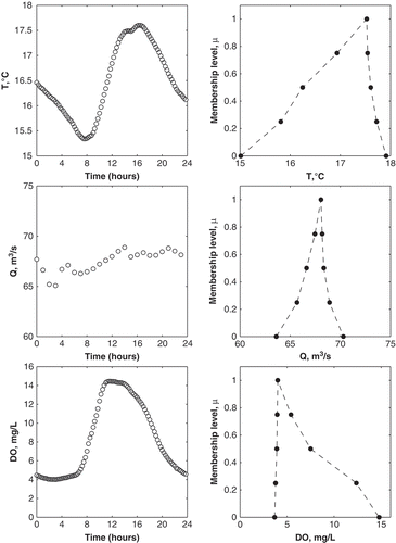
The algorithm described above was used to develop the fuzzy numbers T̃, Q̃, and DÕ corresponding to the crisp data T, Q and DO, respectively, for the 2006, 2007 and 2008 datasets. An example of the observed and fuzzy number version of each variable is illustrated in Fig. 3. Note that convention is followed, by connecting the dots in the right-hand figures with straight dashed lines. Technically speaking, the membership functions developed using the algorithm described above is a discrete process, and does not calculate, nor assume, that the values of µ(X) between the selected points (at µ = 0, 0.25, 0.50, 0.75 and 1) are on a straight line. The algorithm only guarantees that the function is monotonically increasing, as required by the definition of a fuzzy number. In many applications, especially those using triangular membership functions, using two points (at µ = 0 and µ = 1), it is assumed that the function is continuous and linear at all X and µ. The results from this analysis challenge this concept and are clearly illustrated in Fig. 3. Had the typical triangular approach been used, a straight line between the kernel value and the two support values would result in a membership function drastically different from those generated here. This difference is pronounced when it is assumed that the triangular membership functions are symmetrical, i.e. the left and right bounds are equidistant from X_M. Thus, if fuzzy numbers are to be incorporated into physically-based or data-driven models, it is important to accurately portray the prevailing ‘fuzziness’ in the data (Peters 1994). The algorithm proposed here arguably develops a more appropriate fuzzy number representation of uncertain environmental data compared to typical triangular fuzzy numbers.

Fig. 3 Comparison of T, Q and DO observations on 12 September 2006 and their transformations into fuzzy numbers. Note that on the right column, the symbols correspond to µ = 0, 0.25, 0.50, 0.75 and 1, i.e. the selected membership levels used for this research.

2.3 Fuzzy linear regression methods

In the following sections, three fuzzy linear regression methods are defined: the Tanaka method (Tanaka et al. 1982), the Diamond method (Diamond 1988) and a proposed new method. A short derivation of each method is provided, followed by a description of their application to predict DÕ.

2.3.1 The Tanaka method

This method for fuzzy regression is a linear programming problem, formulated as follows (from Tanaka et al. 1982). Given a set of crisp observations x_i and y_i (i = 1, 2, ..., N), a fuzzy equation is required to predict a symmetrical triangular fuzzy number Z̃: {z, z – e, z + e}, where:

(2)

where Ã₀, Ã₁ and Ã₂ are fuzzy number coefficients, defined as {A_j, A_j – c_j, A_j + c_j}, where A_j is the kernel and c_j is the half-width of the support of Ã_j, for j = 0, 1, 2. In other words, the support of Ã_j is defined by [A_j – c_j, A_j + c_j]_α=0. The objective of this fuzzy linear regression method is to minimize the fuzziness J (or as originally referred to, the ‘vagueness’) of the system, which is defined as:

(3)

subject to c_j ≥ 0 and:

(4)

In equation (4), H is a user-defined variable referred to as the h-certain factor. This factor, which is a membership level, restricts the amount of data being used in the regression problem. For example, if H = 1, the problem is to minimize J, only considering the crisp values of Z̃_i, i.e. where µ = 1. As H is reduced, more variability is introduced into the problem, until H = 0, where the full triangular fuzzy data for Z̃_i is being used.

High values of H mean that less uncertainty is incorporated into the regression model. This means that the resulting regression equation will not be able to propagate the uncertainty that exists in the observed data. Essentially, H can be seen as another constraint in the problem: J is to be minimized subject to the constraint of the degree of membership fit and the constraints in equation (4) (Kahraman et al. 2006). By specifying H, the linear problem is trying to minimize the residual between the observed and predicted equations, for only data at membership levels equal to or above the cut-off H.

This method has drawn criticism since it was introduced; the key shortcoming being that least-squares is not utilized and, thus, the problem does not reduce to crisp regression if crisp parameters are used (Diamond 1988, Chang and Ayyub 2001). In essence, this method has replaced the random error component with the fuzzy error component, rather than combining the two. Another issue is that, as the number of observations increases, the constraints and, hence, the amount of computation, increases proportionally (Chang and Ayyub 2001). Also, the results of this technique are dependent on a number of factors: the symmetry assumptions of µ, the value of H used, and the choice of the fuzziness criterion J (which may be defined in a number of different ways, e.g. the sum, mean or maximum of the c_j) (Bárdossy 1990, Bárdossy et al. 1990, Chang and Ayyub 2001). Thus, the success of the model is directly influenced by the selection of these parameters, which are selected specifically to conform to the application, rather than a universal approach, as is expected of regression techniques (Bárdossy 1990). Another limitation of the Tanaka model is that the regressors are required to be crisp. However, even if the model is adapted to use fuzzy regressors (Hojati et al. 2005), the fundamental problems with the model described above are not resolved.

2.3.2 The Diamond method

A key feature of this method, developed by Diamond (1988), is that it incorporates least-squares, which was a key shortcoming in the Tanaka method. A number of other fuzzy regression techniques that use least-squares with linear or quadratic programming have also been developed. These include the maximum compatibility method (Celmiņš 1987) and the minimum fuzziness method (Savic and Pedrycz 1991). Although each of these methods has its advantages, only the Diamond method is discussed here in detail.

In the Diamond method the objective is to minimize D² (a metric defined as the distance between fuzzy numbers) in the least-squares sense, and to determine the regression coefficients as a linear problem. Of the three models described by Diamond (1988), the method that incorporates fuzziness in the input, output and one coefficient is extended to be applicable to cases with multiple regressors and non-symmetrical fuzzy numbers. This is described below.

Given a set of fuzzy observations X̃_i: {x, x^L, x^R}_i and Ỹ_i: {y, y^L, y^R}_i, (i = 1, 2, ..., N) a fuzzy equation is required to predict a triangular fuzzy number Z̃: {z, z^L, z^R}, with:

(5)

where the coefficient Ã₀ {A₀, A₀^L, A₀^R} is a triangular fuzzy number, and the coefficients a₁ and a₂ are crisp numbers. The objective of the fuzzy least-squares problem proposed by Diamond is:

(6)

where

(7)

A solution for this problem can be found by calculating the associated normal equations for equation (6), for the four cases: when a₁ ≥ 0 and a₂ ≥ 0, a₁ < 0 and a₂ ≥ 0, a₁ ≥ 0 and a₂ < 0, or a₁ < 0 and a₂ < 0. The derivation of the solution is trivial and is not shown here. A key difference between this method and the Tanaka method is that, along with the output observations Z̃_i, the input values X̃_i and Ỹ_i are also fuzzy, though limited to triangular fuzzy numbers. However. this approach prevents the coefficients a₁ and a₂ from being fuzzy, due to the necessity of linearity of µ (Diamond 1988). This method essentially defines a metric to express the deviation between two fuzzy numbers, Z̃ and Ã₀ + a₁X̃ + a₂Ỹ, and then minimizes this deviation in a least-squares sense. The implication of this method is that if the error between each corresponding element of the two fuzzy numbers can be simultaneously minimized, then the overall distance D² is also minimized. Kao and Chyu (2003) modified this method to allow the regressors and regressand to be non-triangular membership functions, but kept the coefficient crisp.

A key difference between this method and the Tanaka method is that when crisp data are used, the minimization problem reduces to a conventional least-squares regression problem (Kao and Chyu 2003). By allowing the constant coefficient A₀ to be fuzzy, the random and fuzzy errors are both represented (to an extent). In addition, the h-certain factor does not need to be specified, as the method only relies on the support and the kernel, assuming µ to be triangular.

The majority of research focuses on fuzzy regression systems where not all parameters, i.e. regressor, regressand and coefficients are all fuzzy at once. Typically the model coefficients are crisp and the input and output data are fuzzy (Yang and Lin 2002, Kao and Chyu 2003, Bargiela et al. 2007). However, as noted earlier, the vagueness in a system may be caused by a combination of both measurement error and the indefiniteness of model parameters (Lee and Chen 2001). This combined fuzziness is common when observations are from uncontrollable or uninfluenced sources, as is the case in hydrological and environmental data (Lee and Chen 2001). A consequence of using fuzzy numbers to represent each of the three parameters is that their multiplication results in an increase in the spread of predicted data. In some applications this is seen as unfavourable, since specificity is highly favoured. In contrast, when the objective is to be able to define the maximum map of possibilities, this larger spread is favourable. Further, a possibility–probability transform can be used to convert the uncertain predicted data into a pdf that determines the chance of these outlying data to occur. Thus the ‘correct’ form for a fuzzy regression equation is dependent on the nature of the system being modelled and the nature of the input and output data (Bisserier et al. 2009).

2.3.3 A proposed new method

A method for fuzzy linear regression is proposed, which is an extension of the Diamond method described above. This proposed method is designed to be suitable for the required application, i.e. predicting fuzzy DO, using fuzzy input parameters and fuzzy regression coefficients. This application has additional requirements that have not been addressed in current literature (Yang and Lin 2002, Nasrabadi and Nasrabadi 2004, Hojati et al. 2005, Chachi et al. 2011): specifically that these fuzzy numbers are not limited to the triangular L-R types, µ is not restricted to symmetric functions and each variable may have distinctly shaped µ. In addition, the method should be appropriate for less general fuzzy numbers with discrete membership functions directly created from observed data via a probability–possibility transformation. The proposed method is outlined below:

Given a set of fuzzy observations X̃_i and Ỹ_i, and their corresponding membership functions, µ(X_i) and µ(Y_i), for (i = 1, 2, ..., N) a fuzzy equation is required to predict a fuzzy number Z̃ defined by µ(Z_i), where:

(8)

and the coefficients Ã_j (j = 0, 1, 2) are fuzzy numbers. The objective is to solve the following least-squares problem:

(9)

where

(10)

Note that d² in equations (9) and (10) is not the same as D² in equation (7). This ‘distance’ now measures the sum of the squared-deviations of the observed and predicted (Z̃) crisp intervals , for all α-cuts between µ = 0 and µ = 1. To calculate d², the intervals at µ = 0, 0.25, 0.50 and 0.75 are decomposed into its left and right bounds, whereas the interval at µ = 1 (which cannot be decomposed into left and right values) is left as is:

(11)

Note that in equation (11), the values of α used are not limited to 0, 0.25, 0.50 and 0.75, but can be any set of values, provided that the interval at µ = 1 is separated. Using equation (11), the minimization problem is then redefined as:

(12)

Equation (12) is derived from the fact that the minimum total d² results when the square deviation is a minimum at each α-level. Similarly, at each α-level, d²_α is minimum when both the left (d²_α^L) and right (d²_α^R) values are minimum. Thus, equation (12) can be solved by the usual procedure of deriving a solution from the normal equations, resulting in:

(13a)

(13b)

(13c)

where X_α^L, X_α=1 and X_α^R are matrices of the left, kernel and right bound observations of the regressors, X̃ and Ỹ, respectively, at each α. The terms β^L_α, β_µ=1 and β^R_α are vectors of coefficients Ã_j^L_α, Ã_j|µ=1 and Ã_j^R_α, respectively, for j = 0, 1, 2, at each α, and y^L_α, y_µ=1 and y^R_α are vectors of the left, kernel and right bound observations of the regressand Z̃, at each α. These equations result in the following system of equations:

(14)

where X is a matrix of each X_α^L, X_µ=1 and X_α^R along the diagonal and zeros everywhere else, and β and y are vectors of the corresponding β_α and y_α. Equation (14) is thus solved for β, which gives the values at required membership levels for each fuzzy coefficient Ã₀, Ã₁ and Ã₂.

2.4 Model implementation and comparison

The 2006 and 2007 datasets of T̃, Q̃, and DÕ (the fuzzy versions of observed T, Q and DO), were used to construct each of the three fuzzy linear regression models. The 2008 dataset was used for model verification. It should be noted here that the logarithm of Q was used in each case. The models were implemented in MATLAB (version 2012b).

Since the Tanaka method requires crisp values for the regressors T and Q (see equation (2)), values of T̃ and Q̃ at µ = 1 were used. Also, the method required the regressand DÕ to be a symmetrical, triangular fuzzy number; thus, values of DÕ at µ = 0^L, µ = 0^R and µ = 1 were used to define DÕ as {DO_µ=1, DO_µ=0^L, DO_µ=0^R}. Note that for symmetry DO_µ=0^L must equal DO_µ=0^R; thus, the larger of the distances between each support and the kernel was used. Further analysis was conducted using four different values of H: 0, 0.25, 0.50 and 0.75. Results are only presented for H = 0.25, as higher values do not capture enough of the observed variability, while lower values (i.e. H = 0) are highly uncertain, as explained in Section 2.3.1. The Diamond method requires the regressors and regressand to be triangular fuzzy numbers, thus values of T̃, Q̃, and DÕ at µ = 0^L, µ = 0^R and µ = 1 are used to define a three-element fuzzy number for each variable. For the proposed method, the fuzzy numbers for each variable are represented at five α-levels, corresponding to µ = 0, 0.25, 0.50, 0.75 and 1; these values were selected to give a complete representation of the observed fuzzy number. In each model (equations (2), (5) and (8)) the coefficient Ã₁ was associated with T̃, and Ã₂ was associated with Q̃.

The results from model construction and verification were evaluated using the Nash-Sutcliffe model efficiency coefficient, E, defined as:

(15)

where z_i is the observed value, ẑ_i is the predicted value, z_m is the mean of the observed values of the regressand, and N is the total number of observations. The value of E was first calculated by grouping z_i at each µ together and grouping ẑ_i at each µ together. This meant that for the Tanaka and Diamond methods, the values of z_i and ẑ_i at µ = 0^L, 0^R and 1 were combined into one vector, while for the proposed method, their values at µ = 0, 0.25, 0.50, 0.75 and 1 were combined into one vector. In addition, for the Tanaka and Diamond methods, values of z_i and ẑ_i at µ = 0.25, 0.50, and 0.75 were interpolated (treating the membership function as a linear relationship). These data were then used to estimate E individually at each µ = 0, 0.25, 0.50, 0.75 and 1, and compared with the results from the proposed method at the corresponding membership levels. Similarly, the root mean square error (RMSE, equation (16)) was calculated for each method, with the data at each membership level combined together. In addition, RMSE was calculated at µ = 0, 0.25, 0.50, 0.75 and 1, using the interpolated data described above, for the Tanaka and Diamond methods, and then summed to give an overall total error for each method. The objective of doing this was to demonstrate the difference between errors when using triangular membership functions and when using higher resolution membership functions (as is done in the proposed method).

(16)

The Akaike information criterion (AIC, equation (17)) is also calculated for each method, grouping all the data together, and as a sum at each membership level, as described for RMSE:

(17)

where N is the total number of observations, RMSE is calculated by equation (16), and k is the number of parameters to be estimated in the models. Lastly, the metric D² developed by Diamond (1988) and defined in equation (7), along with the proposed new metric, d² (defined in equation (11)), were also calculated for each method. These metrics were used to define the objective function of the minimization problem and thus, are evaluated to compare the efficacy of each method.

3 RESULTS AND DISCUSSION

The coefficients for the three regression models were calculated and their values illustrated in Fig. 4. The Tanaka model, which used crisp input observations (T and Q), and fuzzy output observations (DÕ), calculated a crisp value for Ã₀, i.e. c₀ = 0, and symmetric triangular membership functions for the fuzzy coefficients Ã₁ and Ã₂. This implies that the best fit of the regressors to the fuzzy regressand, as defined by the criterion J, did not require any uncertainty to be present in Ã₀. The Diamond method used fuzzy input and output observations and had a fuzzy Ã₀ and crisp a₁ and a₂ (as defined by the constraints listed in Section 2.3.2). This resulted in completely different values for the coefficients compared to the Tanaka method. The Tanaka method predicted crisp Ã₀ and fuzzy Ã₁ and Ã₂, while the Diamond method predicted fuzzy Ã₀ and crisp Ã₁ and Ã₂.

Fig. 4 Comparison of the values of the three regression coefficients calculated using the Tanaka method (top), the Diamond method (middle) and the proposed method (bottom).

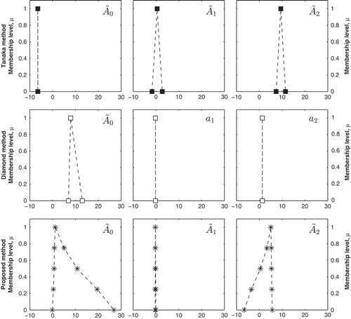
The proposed method, which did not have constraints on whether the coefficients, the regressors or the regressand were fuzzy or crisp, resulted in each coefficient being fuzzy, each with distinct, nonlinear membership functions. This highlights the fact that assuming or selecting linear, or even a symmetric representation, of µ may not be realistic. Also, by removing the crispness constraints on the coefficients, the proposed method produces completely different results compared to both the Tanaka and Diamond methods. The uncertainty, which was represented only in one coefficient in the Diamond method, is now transferred to all three coefficients, with drastically different values. Also, the new approach shows that without having predefined constraints on fuzziness, it still has the ability to generalize to a crisp number if necessary, as is the case for Ã₁, which is nearly fuzzy, with a small support. This shows that the regression model can generalize to crisp linear regression, if crisp regressors are used. By incorporating full system fuzziness, the regression model can provide insight into the physical system, e.g. at low membership levels, when µ = 0^L, i.e. at low Q, the influence of the constant Ã₀ is much lower compared to µ = 0^R when the constant is high (approximately 30, as illustrated in Fig. 4).

The impacts of the different values of the coefficients are illustrated in Figs 5, 6 and 7. Each figure shows a time series plot of observed and predicted DÕ for each method. The observed DÕ is only shown at µ = 0^L and 0^R, whereas the predicted DÕ is shown at µ = 0^L, 0^R and 1. Data at these membership levels were sufficient to illustrate the overall results of each approach; thus data at other µ are not shown. The Tanaka method was not able to capture the observed DÕ at any membership level. This is illustrated by the fact that, in each plot, the predicted values at µ = 0^L and 0^R (black crosses) are three to four times larger than the observed values. Furthermore, the predicted DÕ at µ = 1 (white circle) falls outside the observed DÕ interval at µ = 0 (black circles). Generally speaking, the Tanaka method is not appropriate for this application, as the results from the regression equation do not provide meaningful predictions of DÕ.

Fig. 5 Comparison of observed and predicted DÕ for model construction (2006 data), using (a) the Tanaka method, (b) the Diamond method, and (c) the proposed method. Observed data (black circles) correspond to µ = 0^L and 0^R, while the predicted data are shown for µ = 0^L and 0^R (black crosses) and µ = 1 (white circles).

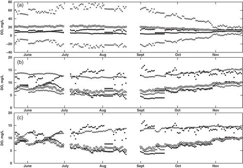
Fig. 6 Comparison of observed and predicted DÕ for model construction (2007 data), using (a) the Tanaka method, (b) the Diamond method, and (c) the proposed method. Observed data (black circles) correspond to µ = 0^L and 0^R, while the predicted data are shown for µ = 0^L and 0^R (black crosses) and µ = 1 (white circles).

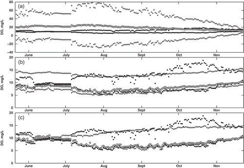
Fig. 7 Comparison of observed and predicted DÕ for model validation (2008 data), using (a) the Tanaka method, (b) the Diamond method, and (c) the proposed method. Observed data (black circles) correspond to µ = 0^L and 0^R, while the predicted data are shown for µ = 0^L and 0^R (black crosses) and µ = 1 (white circles).

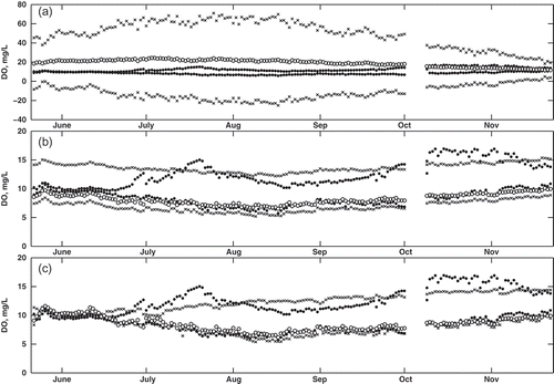
In contrast, both the Diamond method and the proposed new method provide more realistic predictions of DÕ. A major difference between these two methods is immediately evident: although the Diamond method generally follows the observed trend, it cannot replicate the fluctuations in daily observed DÕ. This is illustrated by the band of black crosses, with a near constant width, throughout the entire dataset. However, in the new method, the predicted data follow the transformed observed data much more closely. The predicted supports (black crosses) follow the observed supports (black circles) as the size of the fuzzy interval changes on a daily basis. The reason for this improvement can be traced back to the formulation of the fuzzy regression technique. In the Diamond method, the coefficient a₁ and a₂ are crisp, essentially scaling the observed T̃ and Q̃, and thus limiting the propagation of uncertainty. However, in the new method, the product of the fuzzy coefficients and fuzzy variable produce values that are able to mimic the fluctuations. In addition, the regression problem defined by the Diamond method is not well equipped to predict this type of uncertainty: it is designed to minimize the overall uncertainty (i.e. at µ = 0^L, 0^R and 1 combined). However, the approach of the new method is to minimize the distance on a α-cut interval basis. This ensures that fluctuations at each membership level are matched by the predictions from the regression model. Of note is that the values of DÕ at µ = 1 are skewed closer to values at µ = 0^L than µ = 0^R in both the Diamond and the new method. This mimics the observed data where DO is skewed to lower values (see Fig. 3 for an example). The Tanaka method cannot capture this skewness since it is limited to symmetric fuzzy numbers.

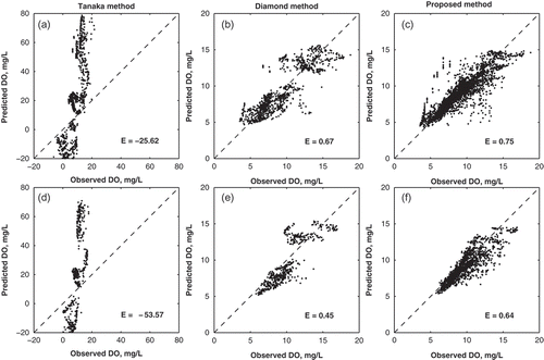
Figure 8 shows plots of observed vs predicted DÕ for each method, for both the construction and verification datasets. Note that these plots include data from all calculated membership levels. The Nash-Sutcliffe coefficient, E, is listed for each method on the figure. The new method has higher values of E compared to the other methods, with E equal to 0.75 and 0.64 for the construction and verification datasets, respectively. The Tanaka method has negative E values for both datasets, confirming that the method is not suitable for this application. The Diamond method fares better than the Tanaka method, with E = 0.67 and 0.45, for the construction and verification dataset, respectively. Of note is that the proposed method slightly under-predicts DO (Fig. 8(c) and (f)), whereas the Diamond method both under- and overpredicts DO (Fig. 8(b) and (e)). Another important point to note is that in the Diamond method (Fig. 8(b) and (e)) the predicted DO has a gap in values between approx. 10 and 12 mg/L in both datasets. This gap represents the data that the method is unable to predict because it cannot capture the daily variability. This gap, and the spread of the data about the one-to-one line, is symptomatic of the shape of the membership functions used (i.e. assumed to be linear in the Diamond method and unconstrained in the proposed method), as well as the representation of uncertainty in each method. It highlights the importance of incorporating system uncertainty (via fuzzy regression coefficients), without which the full spectrum of data cannot be predicted (as seen in the Diamond method).

Fig. 8 Comparison of observed and predicted DÕ, for the construction and verification datasets: (a) and (d) the Tanaka method, (b) and (e) the Diamond method, and (c) and (f) the proposed method. Note that each plot includes values at all membership levels.

Figure 9(a) shows the values of E calculated for the Diamond and the proposed methods at each membership level. Results for the Tanaka method are not included since the method substantially underperformed compared to the other two, and would plot outside the axis limits presented in Fig. 9. Note that for the Diamond method, values at µ = 0.25, 0.50 and 0.75 were calculated using the linearly interpolated predicted values, described in Section 2.4. The figure illustrates that both methods have higher E when predicting the lower values (i.e. left bound) of DO, which are the values of interest in risk analysis. Both models are less accurate when predicting high DO concentrations. Note that in all but two cases (at µ = 0.75^R and 0.50^R for the verification dataset), the proposed method has higher E values compared to the Diamond method, and this trend is consistent in both the construction and verification datasets. For the proposed method, E was calculated to be less than 0.2 on two occasions: at µ = 0.75^R and 0.50^R (for the verification dataset). In comparison, the Diamond method, E was below 0.2 on 12 occasions: at µ = 0.50^R, 0.25^R and 0^R (for the construction dataset) and at all membership levels for the verification dataset. This shows that the proposed method is superior to the Diamond method, even at a lower performance level (i.e. when E < 0.2). The lower E values of the proposed method, at µ = 0.75^R and 0.50^R for the verification data, are a consequence of the method used: it does not suggest a flaw in the new approach, in fact the opposite. Since each α-cut interval is calculated independently for the proposed method, the predicted values reflect the highly variable nature of the daily data at each α-cut, which the Diamond method does not attempt to reproduce. This is also reflected in the RMSE calculations discussed below. Similarly, the low E (<0.2) of the proposed method at the two aforementioned membership levels are not a reflection of overall model performance, nor related to the performance at other membership levels. Note that the Nash-Sutcliffe coefficient was not developed to measure the efficiency of models using fuzzy numbers; nonetheless, it has been presented here for comparison purposes though it may not be a suitable performance measure. Since a fuzzy number is a set of values, all analyses should be conducted using the entire set rather than values at individual membership levels. Thus, the ‘mean’ value required to calculate E at individual membership levels, does not represent the ‘mean’ of a series of fuzzy numbers, as it would for crisp numbers. Thus additional error terms are explored below for comparing model performance.

Fig. 9 Comparison of (a) Nash-Sutcliffe coefficient and (b) RMSE for the Diamond and proposed methods, calculated at µ = 0, 0.25, 0.50, 0.75 and 1.

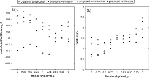
Figure 9(b) shows the RMSE values calculated at each membership level for the Diamond and proposed method. Again, in calculating the RMSE for the Diamond method, interpolated values are used for µ = 0.25, 0.50 and 0.75. The RMSE values increase from the left bound to the right bound (i.e. from µ = 0^L to µ = 0^R). However, this is not reflective of a decrease in performance, but is due to the fact that right bound values are associated with higher values of DO, due to the skewed nature of the data. In general, the new method has lower RMSE than the Diamond method for both datasets, particularly for the left bound (or low DO) data.

Table 1 lists the results of other model comparison criteria, including RMSE, AIC and D². The RMSE was first calculated by combining data at all membership levels for each method. The proposed method had lower RMSE in each case. The Total RMSE, which is the sum of RMSE presented in Fig. 9(b), is also presented in Table 1 and is lower for the proposed method compared to the other two. Similarly, the results for AIC and Total AIC are listed: in both of these cases, the proposed method has a lower AIC. The significance of these results is that when nonlinear membership functions are used to represent the predicted DÕ, then the errors between it and the observed DÕ at the intermediate membership levels are lower compared with assuming linear membership functions.

Table 1 Summary of model performance criteria for each method.

	Tanaka method		Diamond method		Proposed method
	Construction	Verification	Construction	Verification	Construction	Verification
RMSE (mg/L)	27.05	26.40	1.85	1.82	1.35	1.23
Total RMSE (mg/L)	170.57	165.84	14.43	13.65	11.47	10.62
AIC (-)	1169	584	220	108	107	39
Total AIC (-)	8531	4261	1437	659	574	264
Total D^2 (mg/L)^2	2195	2090	10.29	9.94	6.25	4.85

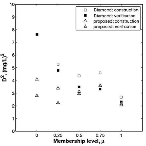
The bottom row of Table 1 shows the calculated metric D² (using equation (7)); D² was calculated for the each predicted DÕ, summed, then divided by the length of the datasets. The results show that the proposed method outperforms the Diamond method, even when using the minimization criteria of the latter. The proposed method had lower values of D² for both the construction and verification datasets. Similarly d² was calculated using equation (11), at µ = 0, 0.25, 0.50, 0.75 and 1. The results of these calculations are shown in Fig. 10, which shows that the new method outperforms the Diamond method. The d² values of the proposed method are lower at each membership level for both the construction and verification datasets. In fact, the difference between the two is greatest at µ = 0, suggesting that the Diamond method is not suitable to model low or high DO. In addition, the results confirm that assuming a linear membership function to determine the values of DÕ at µ = 0.25, 0.50 and 0.75 is not appropriate, as this produces high errors compared to the nonlinear functions used in the new method.

Fig. 10 Comparison of d² for the Diamond and proposed methods calculated at µ = 0, 0.25, 0.50, 0.75 and 1.

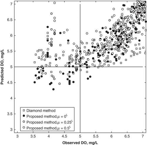
An implication of the differences in results from the methods is illustrated in Fig. 11. The figure shows observed vs predicted data points for the Diamond and the proposed methods, concentrating specifically on the days where there is a possibility of low DO. As previously shown, the Diamond method is unable to capture the day-to-day variability in DO (Figs 5–7), and has higher errors corresponding to low DO values. A result of this inflexibility is that the method predicts fewer days with a possibility of low DO compared to the proposed method. In the example shown in Fig. 11, at µ = 0^L, the Diamond method predicts that there is a possibility of low DO (specifically that DO < 5 mg/L) on 7 days, compared to 28 occurrences with the new method. This difference is pronounced at higher µ: at µ = 0.25^L and 0.5^L, the new method predicts 16 and 4 days, respectively, where DO < 5 mg/L, compared to zero occurrences at both µ for the Diamond method. In addition, the Diamond method overestimates DO at µ = 0^L, when the DÕ is observed to be less than 5 mg/L, as illustrated in Fig. 11. These differences highlight two major results of this research: (a) that the proposed fuzzy regression method can predict DÕ with lower error, and (b) that its nonlinear membership functions improve low DO predictions. Furthermore, the advantage of using fuzzy numbers rather than crisp numbers can be highlighted here as well. Had only crisp observations (µ = 1) been used for this analysis, the linear regression equation would not have predicted any days to have a possibility, or probability, of low DO for the same dataset illustrated in Fig. 11.

Fig. 11 Comparison of observed and predicted DÕ for the Diamond and proposed methods, using the model construction dataset. The Alberta guideline for low DO (5 mg/L) is highlighted.

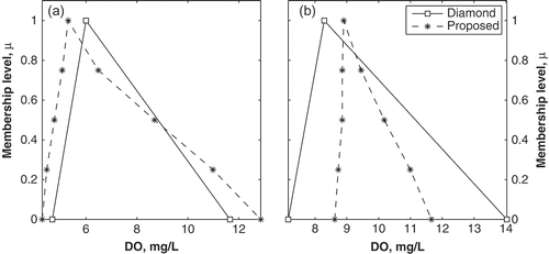
Lastly, to illustrate the difference between the results of the two methods, the membership functions of predicted DÕ are shown in Fig. 12 for one day in 2006 and another in 2007. The functions clearly show that the proposed method does not follow the linear or triangular pattern, typically used to represent fuzzy numbers in environmental data. It is worth highlighting again that, for the proposed method, although the values at each membership level are connected with a straight, dashed line, this does not assume that the values between the selected µ follow the line (i.e. a linear relationship), as is assumed in the Diamond method. Lastly, Fig. 12 also shows that the support of DÕ for the proposed method is more flexible, in that it can match the observed changes in daily DO variation, whereas the Diamond method is less sensitive to change. This is a direct result of how the proposed regression method was designed.

Fig. 12 Comparison of membership function shapes for the predicted DÕ for (a) 23 July 2006 and (b) 22 May 2007.

4 conclusion

A new fuzzy linear regression method is proposed in this paper. The method builds on two previously defined fuzzy linear regression methods (namely, the Tanaka and Diamond methods) and is compared to these to evaluate its performance. Data of DO, Q and T from the Bow River in Calgary, Alberta, Canada were used to demonstrate the performance of the model. First, an algorithm was developed to apply a probability–possibility transformation that converts the observed data into fuzzy numbers. The transformation was able to represent the skewness in the observed data. The fuzzy data were then used to test the three fuzzy linear regression methods, to predict fuzzy DO using fuzzy Q and T as the regressors.

In general, the proposed new method was shown to be superior to the existing methods, as it was able to represent both random and non-random uncertainty in the system, by using fuzzy regressors, regressand and fuzzy coefficients. The new method was able to generate distinct nonlinear membership functions for each regression coefficient. The higher performance of the new method compared to the other two, suggests that linear or symmetric representation of uncertainty (i.e. µ) in the coefficients may not be realistic. The new method also showed that it has the ability to reduce to crisp regression if necessary, a key requirement for fuzzy linear regression methods. This type of fuzzy linear regression approach has the ability to provide insight into physical system.

Comparing the three methods, the proposed method can model the daily fluctuations in DO variability more precisely and accurately compared to the other two methods. This is due to the way the regression system is set up, where the residuals between the observed and modelled data are minimized on an α-cut interval basis collectively. One of the major advantages of this approach is that the skewness of the observed DO can be modelled effectively, giving a tool to predict low DO and other environmental data that are typically skewed. This advantage is highlighted by the fact that the Nash-Sutcliffe coefficient for the new method is higher than for the other two methods, and this difference is greater at low DO values. The proposed method outperforms the other two methods with lower RMSE and AIC at each µ, and also has lower total RMSE and total AIC. The proposed method outperforms the Diamond method when using the Diamond D² and the proposed d² metric. The difference in performance reflected by d² is greatest at µ = 0, which again suggests that the proposed method is better suited to predicting low DO. The significance of these results is that the new method does not overpredict low DO, as does the Diamond case. In fact, it highlights a larger number of days, where there is a possibility of low DO occurring, compared to the Diamond method. These results can be used by water resource managers to conduct risk assessments for the occurrence of low DO. Future research should focus on extending this approach to nonlinear systems (i.e. where the dependent and independent variables are not assumed to be linearly related). The use of fuzzy numbers (as an uncertain quantity) in artificial neural networks should be explored, specifically for improving the prediction of DO in highly uncertain and complex environments.

Disclosure statement

No potential conflict of interest was reported by the author(s).

Acknowledgements

The authors would like to thank the City of Calgary, Alberta Environment and Dr C. Ryan (Geoscience, University of Calgary) for providing data for this research. The authors are also grateful for the helpful suggestions made by two anonymous reviewers that helped improve the quality of this manuscript.

Additional information

Funding

The authors acknowledge the Natural Sciences and Engineering Research Council of Canada and the University of Victoria for funding this work.

APPENDIX

A Fuzzy numbers

Fuzzy numbers are defined as a fuzzy subset of the real line R, i.e. a continuous mapping from R to the closed interval [0,1]. A fuzzy number à is a convex, normal fuzzy set, that has a piecewise continuous membership function µ(x), such that the elements x₁, x₂, ..., x_m, ..., x_n of Ã, where x₁ < x₂ < ... < x_m ... < x_n, and the following hold true:

• For  the intervals x ϵ (–∞, x₁) and (x_m, ∞), µ(x) = 0, µ(x) monotonically increases between x₁ and x_m and monotonically decreases between x_m and x_n,

• µ(x¹) = µ(xⁿ) = 0 and there exists one element x_m where µ(x_m) = 1; this element is referred to as the mode value or the kernel.

A normal fuzzy set, as mentioned above, simply means that there is at least one element x_i, where µ(x_i) = 1. The convexity constraint means that for any three (or more) elements, x_a, x_b and x_c, where x_a < x_b < x_c, the following holds true (Zhang et al. 2009, Wang et al. 2011):

(A1)

The underlying concept of a fuzzy number is to define an imprecise quantity, thus x_m (i.e. the element where µ = 1) is the value that is closest to the true value being measured, while the values x₁ and x_n (where µ = 0) can be considered the upper and lower limits, beyond which are values that cannot be considered possible values of Ã.

The membership function µ(x) describes the degree of membership or membership level that each element has in a fuzzy set (or number). The functions model the gradual change in membership of an element in a fuzzy set. Typically, triangular (or also referred to as ‘L-R’) membership functions are used. In this case, µ(x) is typically defined at three x_i: µ = 0^L (the left or lower bound), µ = 1 (the kernel) and µ = 0^R (the right or upper bound). A common notation for triangular fuzzy numbers is as follows:

(A2)

where à is a fuzzy number, x_b is the kernel of Ã, and x_a^L and x_c^R are the left and right bounds of Ã. Other shapes for membership functions have also been used, including uniform, trapezoidal and Gaussian shaped functions (Duch 2005, Khan et al. 2013).

B The α-cut and the extension principle

The α-cut technique is a method used to reduce a fuzzy number into a series of nested intervals that contain crisp elements (Zhang et al. 2009, Zhang and Achari 2010b, Wang et al. 2011, 2012). It provides a bridge to connect a fuzzy set to a crisp set. Formally, the crisp set A_α is defined as a set that includes all elements x_i that belong to a fuzzy set à with a membership grade greater than or equal to α, where α ∈ [0,1]. This set A_α, is known as the ‘α-level cut’ or simply the α-cut of Ã. In other words, the set A_α contains all x_i that are members of à at degree of membership of at least µ(x) = α. The ordinary set A_α consists of an interval [x_i^L, x_i^R]_α ∈ A_α at some degree of membership α. The α-cut is described as:

(B1)

The extension principle was introduced by Zadeh (1975) and provides a method for extending crisp mathematical functions to deal with fuzzy quantities. Suppose that a function f acts on a fuzzy number Ã, which is defined by the elements x₁, ..., x_n, and that their corresponding membership levels are µ_Ãx1, ..., µ_Ãxn. The fuzzy number Ñ is generated by f acting on à (i.e. Ñ = f(Ã)) and consists of elements y₁, ..., y_n, where y_i = f(x_i). The corresponding µ describing the membership of elements y_i in Ñ are unaffected by the mapping f, and are given by µ_Ãx1, ..., µ_Ãxn. This principle can be generalized to multiple input fuzzy numbers as:

(B2)

where Ã₁ to Ã_n are a series of fuzzy numbers, x₁ to x_n are their corresponding elements, each with a membership level of µ_Ã1(x₁) to µ_Ã1(x_n), and µ_Ñ(y) is the membership level of y, which is an element in the fuzzy number Ñ, and is generated from a mapping f on the elements x₁ to x_n. The term ‘sup’ is the supremum operator and ‘min’ is the minimum (Zadeh 1975, Dubois and Prade 1980).

This implies that the membership levels of the images of elements are not affected by the function f. This effectively reduces mathematical operations on the fuzzy number Ã, into a series of operations on the ordinary sets A_α (the α-cut of à at µ = α). A number of standardized mathematical operations have been defined to use with fuzzy numbers; the reader is referred to Kaufmann and Gupta (1984) for more details.

C Probability–possibility transformation

In order to represent crisp data as fuzzy numbers, the relationship between possibility and probability is used to transform the data. This transformation is referred to as a probability–possibility transformation (Dubois et al. 1993, 2004, Zhang et al. 2009). It converts a uni-modal probability density function (pdf) p(x) with bounded support to a possibility distribution µ(x). The transformation relates the area under a pdf to a membership value. Details on the theoretical background relating the possibility and probability distributions of a variable are not included here, but can be found in Dubois et al. (1993, 2004), amongst others. The transformation is given by:

(C1)

where the kernel of µ(x) is the mode M of p(x) and f(x) is a mapping where for any x, f(x) = y ≥ M, such that p(x) = p(y). It is subject to the constraint:

(C2)

In simple terms, consider a pdf of x, p(x) that is bounded by two values x_min and x_max. A horizontal cut is made at p(x) = H, resulting in two values of x, x^L = p⁻¹(H) and x^R = p⁻¹(H). The sum of the cumulative probability between x_min and x^L and between x^R and x_max, is some value α. This α is the minimum membership level for all values between x^L and x^R, or in other words represents the interval or α-cut given by A_α = [x^L, x^R]_α. This procedure is repeated for all H, between 0 and max{p(x)}, resulting in a series of α-cuts at different α. These values together define the membership function µ of the fuzzy number Ã:

(C3)

where the symbol ∪ represent the union of all α-cuts.

REFERENCES

- Abebe, A.J., Guinot, V., and Solomatine, D.P., 2000. Fuzzy alpha-cut vs Monte Carlo techniques in assessing uncertainty in model parameters. In: Paper presented at Proceedings of the 4th international conference on hydroinformatics, 23–27 July, Iowa City, IA. Cedar Rapids: University of Iowa, College of Engineering. ISBN-10: 0874141249; ISBN-13: 978-0874141245.
- Alberta Environment Protection, 1997. Alberta water quality guideline for the protection of freshwater aquatic life: dissolved oxygen. Edmonton, Alberta, Canada: Standards and Guidelines Branch, Alberta Environment, Catalogue #: ENV-0.94–OP.
- Alberta Environment River Basins, 2012. Bow River at Calgary [online]. Available from: http://www.environment.alberta.ca/apps/basins/DisplayData.aspx?Type=Figure&BasinID=8&DataType=1&StationID=RBOWCALG [Accessed 5 April 2013].
- Altunkaynak, A., Özger, M., and Çakmakcı, M., 2005. Fuzzy logic modeling of the dissolved oxygen fluctuations in Golden Horn. Ecological Modelling, 189 (3–4), 436–446. doi:10.1016/j.ecolmodel.2005.03.007
- Alvisi, S., et al., 2006. Water level forecasting through fuzzy logic and artificial neural network approaches. Hydrology and Earth System Sciences, 10 (1), 1–17. doi:10.5194/hess-10-1-2006
- Alvisi, S. and Franchini, M., 2011. Fuzzy neural networks for water level and discharge forecasting with uncertainty. Environmental Modelling & Software, 26 (4), 523–537. doi:10.1016/j.envsoft.2010.10.016
- Bárdossy, A., 1990. Note on fuzzy regression. Fuzzy Sets and Systems, 37 (1), 65–75. doi:10.1016/0165-0114(90)90064-D
- Bardossy, A., Bogardi, I., and Duckstein, L., 1990. Fuzzy regression in hydrology. Water Resources Research, 26 (7), 1497–1508. doi:10.1029/WR026i007p01497
- Bargiela, A., Pedrycz, W., and Nakashima, T., 2007. Multiple regression with fuzzy data. Fuzzy Sets and Systems, 158 (19), 2169–2188. doi:10.1016/j.fss.2007.04.011
- Bisserier, A., Boukezzoula, R., and Galichet, S., 2009. An interval approach for fuzzy linear regression with imprecise data. In: J.P. Carvalho, et al., eds. Proceedings of the joint 2009 international fuzzy systems association world congress & 2009 European society of fuzzy logic and technology conference, 20–24 July, Lisbon. Lisbon: EUSFLAT, 1305–1310. ISBN 978-989-95079-6-8.
- Celmiņš, A., 1987. Least squares model fitting to fuzzy vector data. Fuzzy Sets and Systems, 22 (3), 245–269. doi:10.1016/0165-0114(87)90070-4
- Chachi, J., Taheri, S.M., and Pazhand, H.R., 2011. An interval-based approach to fuzzy regression for fuzzy input-output data. Paper presented at 2011 IEEE International Conference on Fuzzy Systems, Taipei. Taiwan: IEEE, 2859–2863. doi:10.1109/FUZZY.2011.6007457
- Chang, Y.-H.O. and Ayyub, B.M., 2001. Fuzzy regression methods—a comparative assessment. Fuzzy Sets and Systems, 119 (2), 187–203. doi:10.1016/S0165–0114(99)00091–3
- Chen, Z., Huang, G.H., and Chakma, A., 2003. Hybrid fuzzy-stochastic modeling approach for assessing environmental risks at contaminated groundwater systems. Journal of Environmental Engineering, 129 (1), 79–88. doi:10.1061/(ASCE)0733-9372(2003)129:1(79)
- Di Baldassarre, G. and Montanari, A., 2009. Uncertainty in river discharge observations: a quantitative analysis. Hydrology and Earth System Sciences, 13 (6), 913–921. doi:10.5194/hess-13-913-2009
- Diamond, P., 1988. Fuzzy least squares. Information Sciences, 46 (3), 141–157. doi:10.1016/0020-0255(88)90047-3
- Dou, C., et al., 1997. Numerical solute transport simulation using fuzzy sets approach. Journal of Contaminant Hydrology, 27 (1–2), 107–126. doi:10.1016/S0169-7722(96)00047-2
- Dubois, D., et al., 2004. Probability-possibility transformations, triangular fuzzy sets, and probabilistic inequalities. Reliable Computing, 10, 273–297. doi:10.1023/B:REOM.0000032115.22510.b5
- Dubois, D. and Prade, H., 1980. Fuzzy sets and systems: theory and applications. New York, NY: Academic Press.
- Dubois, D. and Prade, H., 1988. Possibility theory: an approach to computerized processing of uncertainty. New York, NY: Plenum Press.
- Dubois, D., Prade, H., and Sandri, S., 1993. On possibility/probability transformations. In: R. Lowen and M. Roubens, eds. Fuzzy logic. Dordrecht, Netherlands: Kluwer Academic Publishers, 103–112.
- Duch, W., 2005. Uncertainty of data, fuzzy membership functions, and multilayer perceptrons. IEEE Transactions on Neural Networks, 16 (1), 10–23. doi:10.1109/TNN.2004.836200
- Environment Canada Water Office, 2013. Bow River at Calgary [online]. Available from: http://www.wateroffice.ec.gc.ca/graph/graph_e.html?stn=05BH004 [Accessed 5 April 2013].
- Freissinet, C., Vauclin, M., and Erlich, M., 1999. Comparison of first-order analysis and fuzzy set approach for the evaluation of imprecision in a pesticide groundwater pollution screening model. Journal of Contaminant Hydrology, 37 (1–2), 21–43. doi:10.1016/S0169-7722(98)00163-6
- Giusti, E. and Marsili-Libelli, S., 2009. Spatio-temporal dissolved oxygen dynamics in the Orbetello Lagoon by fuzzy pattern recognition. Ecological Modelling, 220 (19), 2415–2426. doi:10.1016/j.ecolmodel.2009.06.007
- Guan, J. and Aral, M.M., 2004. Optimal design of groundwater remediation systems using fuzzy set theory. Water Resources Research, 40, W01518. doi:10.1029/2003WR002121
- Guyonnet, D., et al., 2003. Hybrid approach for addressing uncertainty in risk assessments. Journal of Environmental Engineering, 129 (1), 68–78. doi:10.1061/(ASCE)0733-9372(2003)129:1(68)
- Han, J.C., et al., 2013. Optimal land use management for soil erosion control by using an interval-parameter fuzzy two-stage stochastic programming approach. Environmental Management, 52, 621–638. doi:10.1007/s00267-013-0122-9.
- Hauer, F.R. and Hill, W.R., 2007. Temperature, light and oxygen. In: F.R. Hauer and G.A. Lamberti, eds. Methods in stream ecology. San Diego, CA: Academic Press, 103–117.
- He, J., et al., 2011. Abiotic influences on dissolved oxygen in a riverine environment. Ecological Engineering, 37 (11), 1804–1814. doi:10.1016/j.ecoleng.2011.06.022
- Hermann, G., 2011. Various approaches to measurement uncertainty: a comparison. Paper presented at 2011 IEEE 9th international symposium on intelligent systems and informatics, Subotica. Serbia: IEEE, 377–380. doi:10.1109/SISY.2011.6034356.
- Hojati, M., Bector, C.R., and Smimou, K., 2005. A simple method for computation of fuzzy linear regression. European Journal of Operational Research, 166 (1), 172–184. doi:10.1016/j.ejor.2004.01.039
- Huang, Y., et al., 2010. A fuzzy-based simulation method for modelling hydrological processes under uncertainty. Hydrological Processes, 24 (25), 3718–3732. doi:10.1002/hyp.7790
- Kahraman, C., Beşkese, A., and Bozbura, F.T., 2006. Fuzzy regression approaches and applications. In: C. Kahraman, ed. Fuzzy applications in industrial engineering. Berlin, Germany: Springer, 589–615.
- Kao, C. and Chyu, C.-L., 2003. Least-squares estimates in fuzzy regression analysis. European Journal of Operational Research, 148 (2), 426–435. doi:10.1016/S0377-2217(02)00423-X
- Kaufmann, A. and Gupta, M.M., 1984. Introduction to fuzzy arithmetic: theory and applications. New York, NY: VanNostrand Reinhold.
- Kentel, E. and Aral, M.M., 2004. Probabilistic-fuzzy health risk modeling. Stochastic Environmental Research and Risk Assessment, 18 (5), 324–338. doi:10.1007/s00477-004-0187-3
- Khan, U.T., Valeo, C., and He, J., 2013. Non-linear fuzzy-set based uncertainty propagation for improved DO prediction using multiple-linear regression. Stochastic Environmental Research and Risk Assessment, 27 (3), 599–616. doi:10.1007/s00477-012-0626-5
- Kim, K.J., Moskowitz, H., and Koksalan, M., 1996. Fuzzy versus statistical linear regression. European Journal of Operational Research, 92 (2), 417–434. doi:10.1016/0377-2217(94)00352-1
- Kumar, V., Schuhmacher, M., and García, M., 2006. Integrated fuzzy approach for system modeling and risk assessment. In: V. Torra, Y. Narukawa, A. Valls and J. Domingo-Ferrer, eds. Modeling decisions for artificial intelligence. Berlin, Germany: Springer, 227–238. doi:10.1007/11681960_23
- Lee, H.T. and Chen, S.H., 2001. Fuzzy regression model with fuzzy input and output data for manpower forecasting. Fuzzy Sets and Systems, 119 (2), 205–213. doi:10.1016/S0165-0114(98)00382-0
- Maskey, S., Guinot, V., and Price, R.K., 2004. Treatment of precipitation uncertainty in rainfall–runoff modelling: a fuzzy set approach. Advances in Water Resources, 27 (9), 889–898. doi:10.1016/j.advwatres.2004.07.001
- McMillan, H., et al., 2010. Impacts of uncertain river flow data on rainfall‐runoff model calibration and discharge predictions. Hydrological Processes, 24 (10), 1270–1284. doi:10.1002/hyp.7587
- Mujumdar, P.P. and Sasikumar, K., 2002. A fuzzy risk approach for seasonal water quality management of a river system. Water Resources Research, 38 (1), 5.1–5.9. doi:10.1029/2000WR000126
- Nasrabadi, M.M. and Nasrabadi, E., 2004. A mathematical-programming approach to fuzzy linear regression analysis. Applied Mathematics and Computation, 155 (3), 873–881. doi:10.1016/j.amc.2003.07.031
- Novák, V., 1989. Fuzzy sets and their applications. Bristol, UK: Adam Hilger.
- Peters, G., 1994. Fuzzy linear regression with fuzzy intervals. Fuzzy Sets and Systems, 63 (1), 45–55. doi:10.1016/0165-0114(94)90144-9
- Pogue, T.R. and Anderson, C.W., 1995. Factors controlling dissolved oxygen and pH in the upper Willamette River and major tributaries. Oregon, USA: US Geological Survey Water Resources Investigations Report 95–4205.
- Porter, D.W., et al., 2000. Data fusion modeling for groundwater systems. Journal of Contaminant Hydrology, 42 (2–4), 303–335. doi:10.1016/S0169-7722(99)00081-9
- Savic, D.A. and Pedrycz, W., 1991. Evaluation of fuzzy linear regression models. Fuzzy Sets and Systems, 39 (1), 51–63. doi:10.1016/0165-0114(91)90065-X
- Shiklomanov, A.I., et al., 2006. Cold region river discharge uncertainty—Estimates from large Russian rivers. Journal of Hydrology, 326 (1–4), 231–256. doi:10.1016/j.jhydrol.2005.10.037
- Shrestha, R.R. and Nestmann, F., 2009. Physically based and data-driven models and propagation of input uncertainties in river flood prediction. Journal of Hydrologic Engineering, 14 (12), 1309–1319. doi:10.1061/(ASCE)HE.1943-5584.0000123
- Shrestha, R.R., Bárdossy, A., and Nestmann, F., 2007. Analysis and propagation of uncertainties due to the stage–discharge relationship: a fuzzy set approach. Hydrological Sciences Journal, 52 (4), 595–610. doi:10.1623/hysj.52.4.595
- Tanaka, H., Uejima, S., and Asai, K., 1982. Linear regression analysis with fuzzy model. IEEE Transactions on Systems, Man and Cybernetics, 12 (6), 903–907. doi:10.1109/TSMC.1982.4308925
- Wang, S., et al., 2011. An interval-valued fuzzy linear programming with infinite α-cuts method for environmental management under uncertainty. Stochastic Environmental Research and Risk Assessment, 25 (2), 211–222. doi: 10.1007/s00477-010-0432-x
- Wang, S. and Huang, G.H., 2012. Identifying optimal water resources allocation strategies through an interactive multi-stage stochastic fuzzy programming approach. Water Resources Management, 26 (7), 2015–2038. doi:10.1007/s11269-012-9996-1
- Wang, S. and Huang, G.H., 2013a. An interval-parameter two-stage stochastic fuzzy program with type-2 membership functions: an application to water resources management. Stochastic Environmental Research and Risk Assessment, 27, 1493–1506. doi:10.1007/s00477-013-0685-2.
- Wang, S. and Huang, G.H., 2013b. A two-stage mixed-integer fuzzy programming with interval-valued membership functions approach for flood-diversion planning. Journal of Environmental Management, 117, 208–218. doi:10.1016/j.jenvman.2012.12.037.
- Wang, S., Huang, G.H., and Yang, B.T., 2012. An interval-valued fuzzy-stochastic programming approach and its application to municipal solid waste management. Environmental Modelling & Software, 29 (1), 24–36. doi:10.1016/j.envsoft.2011.10.007
- Xia, X., Wang, Z., and Gao, Y., 2000. Estimation of non-statistical uncertainty using fuzzy-set theory. Measurement Science and Technology, 11 (4), 430–435. doi:10.1088/0957-0233/11/4/314
- Yang, M.S. and Lin, T.S., 2002. Fuzzy least-squares linear regression analysis for fuzzy input–output data. Fuzzy Sets and Systems, 126 (3), 389–399. doi:10.1016/S0165-0114(01)00066-5
- YSI Environmental, 2012. YSI 5200A continuous multiparameter RAS monitor [Online]. Available from: http://www.ysi.com/media/pdfs/W45-5200A-Continuous-Multiparameter-Monitor.pdf [Accessed 18 April 2013].
- Zadeh, L.A., 1965. Fuzzy sets. Information and Control, 8 (3), 338–353. doi:10.1016/S0019-9958(65)90241-X
- Zadeh, L.A., 1975. The concept of a linguistic variable and its application to approximate reasoning—I. Information Sciences, 8 (3), 199–249. doi:10.1016/0020-0255(75)90036-5
- Zadeh, L.A., 1978. Fuzzy sets as a basis for a theory of possibility. Fuzzy Sets and Systems, 1 (1), 3–28. doi:10.1016/0165-0114(78)90029-5
- Zhang, K., 2009. Modeling uncertainty and variability in health risk assessment of contaminated sites. Thesis (Ph. D.), Department of Civil Engineering, University of Calgary, Calgary, AB, Canada.
- Zhang, K. and Achari, G., 2010a. Correlations between uncertainty theories and their applications in uncertainty propagation. In: H. Furuta, D.M. Frangopol and M. Shinozuka, eds. Safety, reliability and risk of structures, infrastructures and engineering systems. London, UK: Taylor & Francis Group, 1337–1344. doi:10.1201/9781439847657–c20
- Zhang, K. and Achari, G., 2010b. Uncertainty propagation in environmental decision making using random sets. Procedia Environmental Sciences, 2, 576–584. doi:10.1016/j.proenv.2010.10.063.
- Zhang, K., Li, H., and Achari, G., 2009. Fuzzy-stochastic characterization of site uncertainty and variability in groundwater flow and contaminant transport through a heterogeneous aquifer. Journal of Contaminant Hydrology, 106 (1–2), 73–82. doi:10.1016/j.jconhyd.2009.01.003