Comparing expert judgement and numerical criteria for hydrograph evaluation

Abstract

This paper investigates the relationship between expert judgement and numerical criteria when evaluating hydrological model performance by comparing simulated and observed hydrographs. Using a web-based survey, we collected the visual evaluations of 150 experts on a set of high- and low-flow hydrographs. We then compared these answers with results from 60 numerical criteria. Agreement between experts was found to be more frequent in absolute terms (when rating models) than in relative terms (when comparing models), and better for high flows than for low flows. When comparing the set of 150 expert judgements with numerical criteria, we found that most expert judgements were loosely correlated with a numerical criterion, and that the criterion that best reflects expert judgement varies from expert to expert. Overall, we identified two groups of 10 criteria yielding an equivalent match with the expertise of the 150 participants in low and high flows, respectively. A single criterion common to both groups (the Hydrograph Matching Algorithm with mean absolute error) may represent a good indicator for the overall evaluation of models based on hydrographs. We conclude that none of the numerical criteria examined here can fully replace expert judgement when rating hydrographs, and that both relative and absolute evaluations should be based on the judgement of multiple experts.

Editor D. Koutsoyiannis

Résumé

Cet article examine la relation entre jugement expert et critères numériques lorsque l’on évalue les performances de modèles hydrologiques en comparant des hydrogrammes simulés et observés. Une enquête en ligne nous a permis de collecter 150 évaluations d’experts sur un échantillon d’hydrogrammes en hautes et basses eaux. Ces évaluations ont ensuite été comparées aux résultats obtenus à l’aide de 60 critères numériques. Les experts ont été plus fréquemment en accord en termes absolus (en notant les modèles) qu’en termes relatifs (en comparant les modèles), et sur les hautes eaux que sur les basses eaux. La comparaison des 150 jugements d’experts et des critères numériques montre que la plupart des experts sont faiblement corrélés à un critère numérique, et que le critère qui reflète le mieux le jugement expert varie d’un expert à l’autre. Globalement, nous avons identifié deux groupes de dix critères qui reflètent bien l’expertise des 150 participants en basses et hautes eaux respectivement. Un critère commun aux deux groupes (l’algorithme de correspondance des hydrogrammes basé sur l’erreur absolue moyenne) peut représenter un bon indicateur pour l’évaluation globale de modèles basée sur les hydrogrammes. On conclut qu’aucun des critères numériques examinés ne peut remplacer le jugement expert lorsque l’on note des hydrogrammes, et que des évaluations relatives ou absolues devraient être basées sur des expertises multiples.

Key words:

• hydrograph evaluation
• hydrological model
• expert judgement
• efficiency
• numerical criterion
• online survey

Mots clefs:

• évaluation d’hydrogrammes
• modèle hydrologique
• jugement expert
• efficacité
• critère numérique
• enquête en ligne

INTRODUCTION

The issue

Imagine yourself as the technical counsel to the Water Agency. You have been asked to evaluate a modelling study that produced a large number of hydrographs. Hydrographs have been simulated by different models and the agency requires your opinion on the quality of the fit of each model. How should you do it? Here are the options.

Hydrologists and water managers often evaluate the quality of model outputs by visually comparing observed and simulated hydrographs (Chiew and McMahon 1993). Visual evaluation benefits from the knowledge of experts and from their skill and experience, and can be very helpful in providing finely tuned assessments of model accuracy. As an example, Bennett et al. (2013) emphasized the possibility for experts to visually detect “under- or non-modelled behaviour” and evaluate overall performance. Nevertheless, the dependence on the personal experience of an expert can also be seen as a drawback, because it makes the evaluation subjective and may therefore influence its reliability (Houghton-Carr 1999, Alexandrov et al. 2011).

Numerical criteria are often considered more valuable than visual judgement because they are reproducible. However, depending on their formulation, numerical criteria will emphasize certain aspects of the set of analysed values (Perrin et al. 2006, Jachner et al. 2007). Besides, despite their apparent simplicity, the behaviours of numerical criteria remain difficult to fully understand and can exhibit unexpected properties (see e.g. Gupta et al. 2009, Berthet et al. 2010a, 2010b, Gupta and Kling 2011, Pushpalatha et al. 2012). Therefore, numerical criteria should be chosen carefully to correspond to the evaluation objectives (Krause et al. 2005). Today, a large variety of numerical criteria exists. Some authors have suggested combining several complementary criteria to obtain more comprehensive model evaluations (Chiew and McMahon 1993, Krause et al. 2005). Others have advised standardizing evaluation tools to make published studies more consistent in terms of evaluation (Dawson et al. 2007, Moriasi et al. 2007, Schaefli and Gupta 2007, Reusser et al. 2009, Alexandrov et al. 2011, Ritter and Muñoz-Carpena 2013).

Obviously, if you ask your colleagues to help with the job of visual evaluation, or if you use any set of numerical criteria, the result might differ from your own expert assessment. A possible solution would be to select candidates who think the way you do, and/or to select criteria that match your own way of evaluating …, but how can you identify them?

Past experiments relating expert judgement to numerical criteria

Some studies on interdisciplinary modelling processes (such as Kloprogge and van der Sluijs 2002, Kloprogge et al. 2011, Matthews et al. 2011) analysed expert opinions through surveys, videos or interviews. For example, Cloke and Pappenberger (2008) tried to relate the eyeball evaluation and numerical criteria for detecting spatial patterns. However, expert judgement has not been extensively investigated for the purpose of hydrograph evaluation. Visual inspection is considered a full-fledged evaluation technique (Rykiel 1996) and many authors advise combining visual inspection along with other qualitative evaluations with quantitative evaluation techniques (Chiew and McMahon 1993, Mayer and Butler 1993, Houghton-Carr 1999, Pappenberger and Beven 2004, Moriasi et al. 2007, Bennett et al. 2013).

Among these studies, only a few have attempted to relate the two evaluation approaches. Chiew and McMahon (1993) led a survey in which 63 hydrologists were asked to define the visual and numerical criteria they prefer when evaluating a model, and to assess the quality of 112 discharge simulations on 28 catchments. Their analysis resulted in guidelines on how to evaluate hydrographs in absolute terms (perfect, acceptable, satisfactory) depending on the values of several efficiency criteria (Nash-Sutcliffe efficiency, coefficient of determination, bias). Houghton-Carr (1999) compared two expert judgements with results from ten numerical criteria. She contributed in showing evidence of the discrepancies between the qualitative and quantitative methods when ranking hydrological models. No universal criterion, quantitative or qualitative, could be selected from the studied set. More recently, Olsson et al. (2011) asked 12 experts from the Swedish Meteorological and Hydrological Institute (SMHI) to rank model simulations with respect to six visual criteria (overall fit, mean volume, timing, variation, peaks and low flows) on a scale ranging from 1 to 5. On the basis of this survey, the authors characterized the relationship between expert judgement and numerical criteria rating scales and they identified the value ranges of the modified Nash-Sutcliffe criterion considered to be acceptable or good.

Calibration and evaluation methods combining expert judgement and numerical criteria

Acknowledging the possible disagreement between expert judgement and numerical criteria on hydrographs, a few authors have tried to develop calibration methods, visual evaluation techniques, or numerical criteria combining the two approaches.

Boyle et al. (2000) developed a calibration approach that combines manual and automatic methods. From the mathematically acceptable sets of parameters obtained after a search using numerical criteria, a solution is chosen by visual and objective methods. Results obtained with this approach were later compared with results obtained via a fully manual calibration (Boyle et al. 2001). Similarly, the Multi-step Automated Calibration Scheme (MACS) developed by Hogue et al. (2000, 2003, 2006) reproduces the steps hydrologists follow to manually calibrate models.

Pappenberger and Beven (2004) developed a method to evaluate hydrographs by dividing them into box areas and evaluating each box by means of an adequately chosen numerical criterion. With this technique, the expert judgement is integrated when defining the boxes and choosing the numerical criteria to be applied in each of these boxes. Also based on subdivided hydrographs, Zappa et al. (2013) proposed a new visualization of ensemble peak-flow forecasts for an easier evaluation.

In recent years, two numerical criteria were proposed to automatically reproduce the way experts visually evaluate hydrographs. Ehret and Zehe (2011) proposed the Series Distance criterion, in which they paired and compared the timing and amplitude of observed and simulated events on the rising and recession limbs of hydrographs separately using a regular mathematical criterion. Ewen (2011) proposed the Hydrograph Matching Algorithm, which quantifies the distance between simulated and observed hydrographs by means of elastic bands and calculates the minimum energy required to fit the simulated to the observed event.

Scope of the paper

In this article, we aim to clarify the similarities and differences between quantitative and qualitative techniques for the evaluation of simulated hydrographs. The analysis is based on the visual evaluations performed by 150 hydrologists with various backgrounds and experience. From now on, this group of international hydrologists, who agreed to answer the survey and whose characteristics will be described later, will be referred to as ‘experts’. Our objective was twofold: (1) to investigate the similarity between experts’ judgements (who is the closest to me in terms of judgement?), and (2) to look for links between numerical criteria and the judgement of these 150 experts (which numerical criterion is closest to my expert judgement?).

The remainder of this paper is organized as follows: the Methodology section presents the design of the survey, the chosen set of numerical criteria, and the statistical methods applied to compare experts with each other and relate our group of experts to numerical criteria. Then, the results are presented in detail and discussed. Lastly, concluding remarks and tentative recommendations are provided.

Table 1 The r_C value for each criterion and corresponding similarity index, S_C (the meanings of the 60 criteria are detailed in the Appendix).

Criterion	High flows		Low flows		Criterion	High flows		Low flows
	rc	SC^max (%)	rc	SC^max (%)		rc	SC^max (%)	rc	SC^max (%)
AIC	0.92	57.7	1	41.9	MSRE	0.83	53.2	0.85	53.5
AME	0.72	49.6	0.96	40.5	Pdiff	1	45.4	0.95	41.0
Bias	0.44	50.1	0.58	37.5	PI	0.77	51.8	1	40.2
BIC	0.83	57.3	1	41.9	R2	0.94	46.4	1	45.7
CVR	0.91	59.5	1	41.9	R4MS4E	0.88	56.9	0.96	39.4
EI	0.83	59.5	1	41.9	RAE	0.93	59.2	0.93	47.0
EI2	0.79	55.2	0.95	41.2	RBFI	0.96	44.1	1	33.8
EIFDC	0.66	62.2	1	40.0	REMP	1	45.4	0.95	41.0
EILN	0.88	54.4	0.84	56.3	Rmod	0.98	50.4	0.75	32.5
EIparam	0.74	56.3	1	41.9	RMSE	0.91	59.5	1	41.9
EIR	0.89	58.4	1	46.6	RVE	0.44	50.1	0.58	37.5
EIrel	0.83	53.2	0.85	52.5	SEI	0.83	59.5	1	42.0
ESC	0.76	35.3	0.70	46.4	TEST	0.86	42.0	1	40.7
IA	0.70	60.4	0.65	37.5	WR2	0.98	46.5	0.97	38.9
IArel	0.85	52.9	0.98	49.3	EIHF	0.79	56.2	0.83	36.3
KGE	0.75	60.1	0.53	34.8	EILF	0.50	43.8	0.95	54.8
MAE	0.93	59.2	0.93	47.0	FTEI	0.79	47.4	1	32.8
MARE	0.84	55.7	0.96	60.0	MRAF	1	42.5	0.94	41.1
MCE	0.44	50.1	0.60	37.5	RLFD	0.37	33.6	0.97	45.9
MdAPE	0.95	50.6	0.88	62.0	RMLFV	0.84	39.1	0.98	58.2
MEI	0.83	59.5	1	42.0	RMP	0.99	52.6	0.91	33.8
MRE	0.50	40.2	0.60	53.7	RMV	0.97	54.1	1	36.3
MSDE	0.85	47.0	1	36.3	RMVSX	0.84	50.4	1	39.6
MSE	0.83	59.5	1	41.9	VMAE,1	0.94	58.9	0.99	51.4
MSEA	0.77	46.8	0.58	41.3	VNSE,1	0.57	61.6	1	39.0
MSEL	0.66	45.7	0.66	37.7	VNSE,2	0.81	60.0	0.98	42.1
MSEP	0.79	45.4	0.34	36.0	SDv	0.80	57.2	–	–
MSES	0.85	54.9	0.34	37.4	SDt	0.60	40.2	–	–
MSEU	0.92	42.9	1	51.1	SDvt	0.75	51.9	–	–
MSLE	0.88	54.4	0.84	56.3	THREAT	0.93	33.2	0.96	29.0

Table 2 Criteria best matching expert judgement and the associated maximum similarity index values (S_C) in low and high flows, using the optimum ratio value (r_c) (for criteria # and name refer to Appendix).

Rank	High flows			Low flows
	#	Criterion name	SC (%)	#	Criterion name	SC (%)
1	8	EIFDC	62.2	20	MdAPE	62.0
2	55	VNSE,1	61.6	18	MARE	60.0
3	14	IA	60.4	50	RMLFV	58.2
4	16	KGE	60.1	30 9	MSLE EILN	56.3
5	56	VNSE,2	60.0	46	EILF	54.8
6	5	CVR	59.5	22	MRE	53.7
	6	EI
	21	MEI
	24	MSE
	40	RMSE
	42	SEI
7	17	MAE	59.2	31	MSRE	53.5
	36	RAE
8	54	VMAE,1	58.9	12	EIrel	52.5
9	11	EIR	58.4	54	VMAE,1	51.4
10	1	AIC	57.7	29	MSEU	51.1

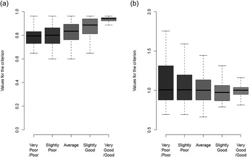
Table 3 (a) Lower quartile, upper quartile and median for V_NSE,1 in high flows and lower quartile, upper quartile and range of quartile distance from optimum for RMLFV in low flows and for each evaluation class. (b) Lower quartile, upper quartile and median for each evaluation class for the Nash-Sutcliffe criterion (EI) and the KGE criterion in high flows.

Qualitative scale	Quartile values for VNSE,1 and median	Quartile values for RMLFV and range of quartile distance from optimum
(a)
Very Poor – Poor	[0.73, 0.83] – 0.79	[0.88, 1.31] – [‒0.12, 0.31]
Slightly Poor	]0.73, 0.87] – 0.80	]0.88, 1.20] – [‒0.12, 0.20]
Average	]0.76, 0.90] – 0.83	]0.88, 1.13] – [‒0.12, 0.13]
Slightly Good	]0.83, 0.94] – 0.89	]0.87, 1.06] – [‒0.13, 0.06]
Good – Very Good	]0.92, 0.95] – 0.94	]0.95, 1.04] – [‒0.05, 0.04]
Qualitative scale	Quartile values for EI and median	Quartile values for KGE and median
(b)
Very Poor – Poor	[0.29, 0.66] – 0.55	[0.55, 0.70] – 0.61
Slightly Poor	]0.43, 0.67] – 0.57	]0.55, 0.70] – 0.66
Average	]0.56, 0.75] – 0.65	]0.61, 0.76] – 0.69
Slightly Good	]0.57, 0.80] – 0.67	]0.66, 0.79] – 0.70
Good – Very Good	]0.65, 0.88] – 0.80	]0.66, 0.90] – 0.82

Fig. 1 Locations of the 29 French catchments for which example hydrographs were selected for evaluation in low-flow (dark grey) and high-flow (light grey) conditions.

Fig. 2 Screenshot showing an example of a displayed hydrograph and the related questions.

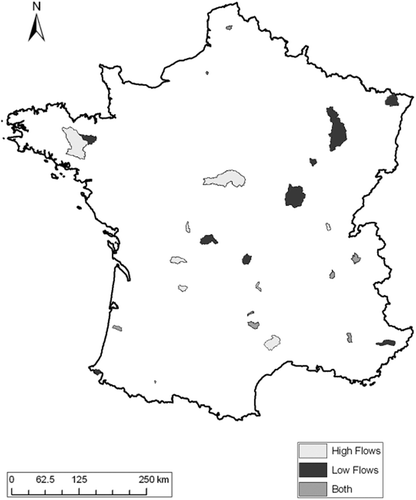
Fig. 3 Evolution of the similarity index for the mean absolute error (MAE) criterion with the ratio value (r_c is the ratio value for which the maximum similarity index S_C^max is reached).

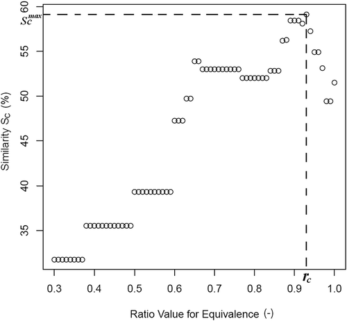
Fig. 4 Information on the experts who took the survey: (a) work status, (b) sectors they work in, (c) work in relation to hydrological modelling, and (d) years of experience in hydrological modelling (from www.surveygizmo.com).

Fig. 5 Hydrographs (a) 26 and (b) 31 as presented in the online survey.

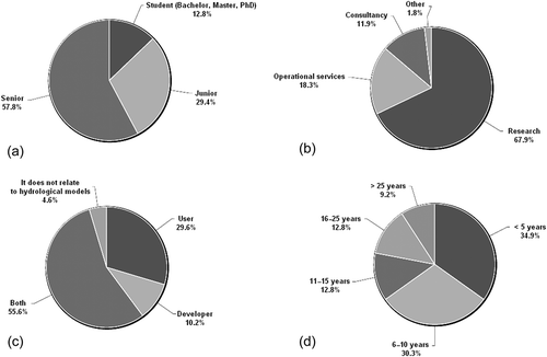
Fig. 6 Distribution of all possible pairs of experts (150 × 149/2 values) according to their similarity in answers for: (a) Question 1 and (b) Question 2.

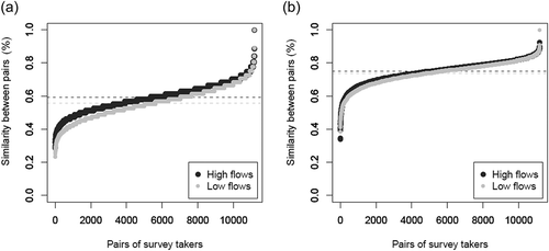
Fig. 7 Ordered leniency scores for the set of participants in evaluation of high and low flows. Dashed lines indicate mean leniency scores for each question. The solid black line indicates the mean of all expert answers for Question 2.

Fig. 8 Box plots of r_c values obtained in high and low flows.

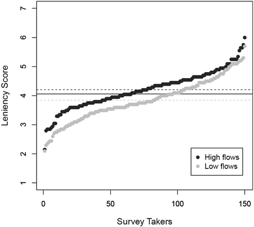
Fig. 9 Matrix of determination coefficients between numerical criteria for the relative evaluation of hydrographs (Question 1).

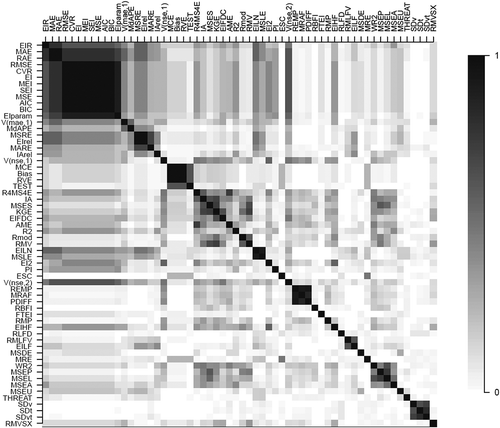
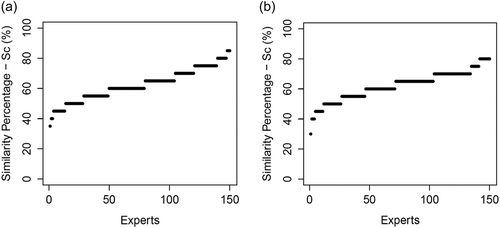
Fig. 10 Spread of participants according to their similarity index to (a) EIFDC in high flows and (b) MdAPE in low flows.

Fig. 11 Number of times each criterion best matches one expert judgement (criterion number corresponds to # in the Appendix).

Fig. 12 Scaled box plots for (a) the V_NSE,1 criterion in high flows and (b) the RMLFV criterion in low flows.

METHODOLOGY

This section presents the design of the interactive survey, the computation of the numerical criteria, and the statistical methods used to analyse the results. A more detailed description is given by Crochemore (2011).

Design of the survey

Here is a way for you—as technical counsel—to assess how your colleagues evaluate hydrographs and how their judgements relate to your own.

The survey was designed using the Survey Gizmo® software (www.surveygizmo.com) and was accessible online from June to August 2011. It was submitted to a large panel of hydrologists both before and throughout the HW06 workshop organized during the IAHS-IUGG conference in Melbourne, in July 2011. The survey consisted of:

1. instructions on how to answer the survey;

2. two sets of 20 hydrographs to be evaluated, focusing on low and high flows respectively; the number of hydrographs was chosen as a compromise between getting a sufficient number of answers to have statistically significant results and not boring the participants; and

3. a form for participants to fill in personal information (work experience, background in hydrology and modelling, etc.) and indicate which aspects of the hydrographs were the most relevant in their visual evaluation.

The survey consisted in visually comparing and rating daily flow hydrographs simulated by various hydrological models. Forty observed hydrographs originating from 29 French catchments (see Fig. 1) were arbitrarily selected from the database built by Le Moine et al. (2007) to provide a variety of hydro-meteorological conditions. They were 1- to 3-month long for high-flow hydrographs and 2- to 5-month long for low-flow hydrographs, to display the full events in each case. To ease visual evaluation, hydrographs focusing on low flows were displayed on a logarithmic scale.

Several daily lumped model structures were used in pure simulation mode (i.e. without any updating) to generate different hydrograph behaviours and shapes: GR4J (Perrin et al. 2003), and simple modified versions of Mordor (Garçon 1996, Mathevet 2005), Sacramento (Burnash 1995), SMAR (O’Connell et al. 1970, Le Moine et al. 2007) and TOPMODEL (Beven and Kirkby 1979, Michel et al. 2003). It is beyond the scope of this article to detail the characteristics of these model structures; however, they were used in previous comparative tests on French catchments and yielded quite reliable results (Perrin et al. 2001, Mathevet 2005, Le Moine 2008).

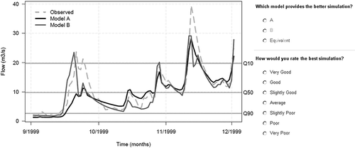
Then, the evaluation of hydrographs was guided by two questions (see example in Fig. 2):

• Question 1 focused on relative model evaluation by model comparison. The expert was asked to select the better of the two hydrographs simulated by models A and B, or to declare them equivalent.

• Question 2 focused on absolute model evaluation by model rating. The expert was asked to rate the simulation considered better in Question 1 on a 7-level scale (ranging from ‘Very Good’ to ‘Very Poor’). This 7-level scale aimed at obtaining fairly precise evaluations.

The idea behind this survey was to collect answers from a large number of hydrologists so as to obtain meaningful results. However, we acknowledge that it is difficult to say whether this sample can be considered a statistically representative sample of the whole community of hydrologists. One reason is that characterizing this community is difficult and definitely far beyond the scope of this study. Hence it was not possible to design a survey answering the usual standards in terms of sampling strategy, as defined by Yates (1981). Therefore, the reader should keep in mind that the results and conclusions presented here are dependent on the characteristics of our sample of experts.

Computation of numerical criteria

You would now like to test numerical criteria in the same way you tested your colleagues, based on the same hydrographs. You wish to identify a single criterion fitting your own judgement and automate the evaluation of your pile of hydrographs.

A number of studies, including those by Smith et al. (2004), Dawson et al. (2007, 2010), Krause et al. (2005), and references therein, were analysed to compile a list of 60 criteria (see Appendix). Although these criteria are not all independent, no prior selection was made based on either correlations or on common uses, e.g. criteria commonly used for high or low flows. Indeed, the aim of the study was to consider as many criteria formulations as possible and try to relate them to expert judgement without a priori considerations that could prove wrong.

Methods to analyse expert judgement

Similarity between experts

Here, we define the similarity between two experts as the number of common answers between them. We transformed answers to the two questions into numerals. For Question 1, the answers corresponding to ‘A’, ‘Equivalent’ and ‘B’ were replaced by 1, 2 and 3, respectively. For Question 2, the range of answers (from ‘Very Poor’ to ‘Very Good’) was replaced by an integer range (from 1 to 7). The similarity D_GF between two experts G and F was computed as:

(1)

where (a_i^G)_i∈[1,N] and (a_i^F)_i∈[1,N] are the answers of experts G and F, respectively, for the N high-flow or low-flow hydrographs evaluated by Question 1 or Question 2; D_max is the maximum possible distance between two experts and is equal to in Question 1 and in Question 2. The similarity for Question 2 is calculated regardless of the answers of the two experts to Question 1, which induces an approximation in the similarity calculation. However, we believe that this does not greatly influence the trends in the results. The similarity criterion scores are within the range [0,1]. A value of 1 indicates that two experts answered exactly the same.

Variability of experts’ answers on each hydrograph

We analysed the variability of answers to the two questions by computing the coefficient of variation for each hydrograph in each case. Using the same numerical scales as previously, we calculated the coefficient of variation for each hydrograph:

(2)

where σ_H is the standard deviation and μ_H is the mean of all expert answers for either Question 1 or Question 2 on hydrograph H. Larger coefficients of variation indicate more dispersed answers.

Leniency score

The leniency score was meant to quantify how demanding the experts were when rating hydrographs. The score is a simple mean of the answers of an expert to Question 2 using the same numerical scale as before (1–7). A systematic Very Poor (Very Good) rating would yield a score of 1 (7), while answers evenly spread over the scale would yield a score of 4. This was called ‘leniency score’ to make its meaning more explicit in the context of this study. Scores were computed for high and low flows separately. Note that in the current investigation, the leniency score obtained for all experts’ answers for both high and low flows is equal to 4.06, i.e. centred on the Average rating.

Methods to compare expert judgement and numerical criteria

Similarity between experts and numerical criteria

The similarity between an expert and a criterion is meant to quantify the number of common answers between the criterion and the expert for Question 1. The similarity index S_J,C (%) between judge J and criterion C is defined as the percentage of common answers and is calculated by:

(3)

with δ_JC,i = 1 if judge J and criterion C have the same answer to Qi and δ_JC,i = 0 if judge J and criterion C have different answers to Qi, and N is the number of high-flow or low-flow hydrographs evaluated. A S_J,C value of 100% means that the criterion and the expert answered identically, while a value of 0% means that they have no common answers. We define the similarity index of criterion C with the whole set of experts S_C as the mean of S_J,C, where J covers the set of all the experts.

Numerical threshold representing equivalent hydrographs in expert judgement

In a relative evaluation (Question 1), the hydrographs should be different enough for the human eye to notice; if not, they are considered equivalent. One may implement statistical tests to evaluate how different two criterion values are, but this may not corroborate what the eye can distinguish. Here, we tried to define by means of criteria what ‘different’ or ‘equivalent’ means for the experts.

Let us consider two simulations provided by models A and B, and C as the numerical criterion, with C_A and C_B for models A and B, respectively. For each hydrograph, we computed the following ratio r to quantify the difference between C_A and C_B:

(4)

with f(err) being a function of the selected model error. The choice to use 1 – C instead of C for criteria written as 1 – f(err) (like the Nash-Sutcliffe efficiency index) is to ensure coherence of results with criteria written as f(err); r falls within the interval If C_A and C_B are close, this ratio will be close to 1; otherwise the ratio will be close to 0. We tried to identify the ratio value (denoted r_c and within the ]0,1] interval) above which simulations A and B can be considered equivalent by experts, i.e. the ratio value that yields the best agreement between experts’ answers and criterion answers:

(5)

For a given criterion, a value of r_c close to 1 means that hydrographs judged as equivalent by experts also have very close criterion values, i.e. the expert judgement and the criterion tend to agree on which hydrographs are equivalent. Conversely, a value of r_c close to 0 means that experts do not distinguish differences between hydrographs whereas criterion values are very different.

Figure 3 shows the evolution of the similarity index with the ratio value in the case of the mean absolute error (MAE). Here, the maximum similarity index is reached when r_c is equal to 0.93, which means that when the ratio of criteria values is larger than 0.93, hydrographs were often considered equivalent by experts. To get general results, the analysis was made using the answers of all experts to Question 1. Results were computed separately for high and low flows.

RESULTS AND DISCUSSION

In this section, we first present preliminary information on the participants and their answers. We then compare the participants with each other by analysing the similarities and differences in their answers. Last, we relate the answers of the participants to numerical criteria.

Preliminary results of the survey

As acknowledged by several authors (Mayer and Butler 1993, Houghton-Carr 1999), the background and experience of experts may have an impact on the way they evaluate model simulations. Thus, it is interesting to analyse the set of participants to understand what the results are representative for.

In total, 150 hydrologists from 79 institutions and 20 countries answered the survey (39 during the IUGG 2011 workshop in Melbourne and 111 via the Internet site). The bulk of participants were typically researchers with large experience in their respective research fields, but relatively less experience in hydrological modelling (see Fig. 4). Operational services and consultancy were also well represented in the survey. Most participants were used to working with hydrological models, as model users but also as model developers.

We then tried to characterize the raw answers. For Question 1, the gap between the number of ‘A’ and ‘B’ answers is variable. For some hydrographs, votes were almost unanimous, e.g. 147 votes out of 150 for model A in hydrograph 26 (Fig. 5(a)). For others, votes were almost equally divided, e.g. hydrograph 31, where votes were shared almost equally for A, B and Equivalent (Fig. 5(b)). Therefore, a wide range of evaluation conditions were gathered in the survey. For Question 2, experts preferred moderate answers (‘Average’, ‘Slightly Good’ and ‘Slightly Poor’) over extreme ones (‘Very Good’ and ‘Very Poor’). Indeed, the number of ‘Average’ answers is about seven times larger than the number of ‘Very Poor’ answers. Also, the answers were distributed quite equally between positive and negative answers. In the survey, experts were asked to assess the importance they gave to six aspects when evaluating the hydrographs, namely: (1) mean flow, (2) timing, (3) magnitude of minimum/maximum values, (4) event duration, (5) slope of the rising limb and (6) slope of the recession curve. For high flows, agreement in rising and recession limbs prevailed and event duration was considered last in ranking the models. For low flows, agreement in recession limbs was the most important, while agreements in rising limbs and event duration were of least importance.

Comparing experts

It is now time for you, as an expert chosen by the Water Agency, to test the trustworthiness of your colleagues with the presented methods. Four levels of similarity can be sought:

1. identify the expert who has the largest number of common answers with you;

2. find out whether your colleagues are more likely to agree with you on a relative or an absolute evaluation;

3. evaluate whether your colleagues are comparably demanding in the absolute evaluation; and

4. study whether they use the same visual criteria as you do.

Similarities at the scale of paired experts

Figure 6 presents the similarity (D_GF) values obtained between all possible pairs of experts (i.e. ) in high and low flows for Question 1 (Fig. 6(a)) and Question 2 (Fig. 6(b)). For each expert, we identified the best matches for each of the two questions. In both questions, similarities are lower in low flows than in high flows. This suggests that the agreement between experts was overall better for the evaluation in high-flow conditions.

We further analysed whether experts who agreed on Question 1 also agreed on Question 2. Since the similarity indices computed for the two questions are not comparable, we ranked for each question the similarity values for all possible pairs of experts from most to least similar. Then we compared for each pair the ranks between the two questions to identify a possible correlation between similarities in Questions 1 and 2. The correlation coefficient of only 0.17 between the ranked similarity values on the two questions indicates that pairs of experts similar in Question 1 are not necessarily similar in Question 2. Therefore, the patterns implied in the relative and absolute evaluations seem independent.

Evaluation of the variability between experts in the two questions

The coefficients of variation of the 40 hydrographs were calculated for the two questions. Then, we applied the Wilcoxon signed-rank test to vectors and to find out for which of the two questions the experts’ responses were more dispersed (corresponding to larger coefficients of variation). The test gave a value of 582 (for the sum of ranks assigned to the differences with positive sign), which indicates that Question 1 tends to yield higher coefficients of variation than Question 2. In addition, the associated p value of 0.02 shows that this difference is significant. Therefore, experts agreed more on Question 2, since their answers are less dispersed.

Experts seem to make choices in a more straightforward way when confronted with ‘Yes/No’ type questions like Question 1 than when confronted with a rating scale that asks for an in-depth appreciation. Thus, a single expert evaluation will be less likely to represent the group of experts when relatively evaluating models and therefore a multi-expert evaluation should be used.

Leniency of the group of experts for the absolute evaluation

Figure 7 presents the distribution of the leniency scores (Question 2) obtained for the 150 experts for high and low flows. The score intends to quantify how demanding experts were, larger values indicating more satisfactory simulations. We observed similar distributions in evaluation of high and low flows, with slightly higher scores in high flows. This could indicate that experts are more demanding in terms of the simulation quality of low flows or that the chosen models performed better in high flows than in low flows. Note that an expert may be demanding because he or she believes that hydrological models can achieve better results than those presented, which denotes optimism. In our case, the experts were equally divided between optimistic and pessimistic attitudes.

After these four steps, you have an idea of how your colleagues evaluate hydrographs compared to the way you do. You did find the perfect candidate to replace you in judging the pile of hydrographs but, unfortunately, after having considered the scale of the task, the expert declines your offer. Thus, you are left with the hydrographs to evaluate and you choose to investigate the second evaluation option: using numerical criteria.

Comparing expert judgement and numerical criteria

You now have a list of 60 numerical criteria to test, in three steps:

1. find out to what extent hydrographs found equivalent by experts are numerically equivalent;

2. identify a set of criteria that provide answers best matching your evaluation; and

3. investigate how the expert assessment scale (ranging from Very Good to Very Poor) can be replaced by a numerical one.

Equivalence between hydrographs in the relative evaluation

For each criterion, we identified the ratio r_c that yielded the best agreement between the evaluations by the criterion and by the experts for Question 1 (see Table 1). For example, a value of r_c = 0.9 means that two simulations with a ratio (see equation (4)) greater than 90% may be considered equivalent by experts.

First, note that the presented r_c values are more robustly determined in high flows than in low flows. Indeed the more ‘Equivalent’ answers we have, the more robust the r_c values are; we received a larger number of ‘Equivalent’ answers in high flows than in low flows: 953 (over the set of 150 × 20 answers) against 775, respectively.

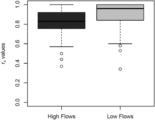
The r_c values range between 0.37 and 1 in high flows and 0.34 and 1 in low flows. However, the distribution of these values is not the same in the two cases (Fig. 8): r_c values tend to be larger in low flows than in high flows and thus tend to better match the notion of equivalence as seen by the expert in low flows. Therefore, if experts want to find the better of two simulations and cannot do so visually, numerical criteria will tend to add more information to their visual evaluation in high-flow cases than in low-flow cases.

In most cases, numerical criteria obtained similar r_c values in high- and low-flow cases. However, in some cases, e.g. overall systematic error (MSES), proportional systematic error (MSEP) or ratio of low-flow deficit (RLFD) (see Appendix), the discrepancy between high- and low-flow cases is drastic. This may indicate that these criteria have very different behaviours in high and low flows, at least when judging between equivalent simulations.

Criteria best matching the expert judgement for the relative evaluation

The analysis aimed to identify the 10 numerical criteria best representing the expert judgement, in evaluation of high and low flows separately, in the case of Question 1 (relative evaluation). We generated individual and general rankings of the criteria using the similarity indices S_J,C and S_C, respectively (see equation (3)). Table 2 shows the top 10 matching criteria in evaluation of low and high flows using r_c values obtained from Table 1. Note that criteria showing high coefficients of determination (see Fig. 9) do not necessarily show the same ranking in Table 2 since their r_c values identified here may differ depending on their formulation. The construction of the r_c values was nonetheless chosen to minimize such discrepancies. Similarity indices between numerical criteria and the group of experts calculated without using r_c values (i.e. considering r_c = 1) can be found in Tables A1, A2 and A3 in the Appendix.

In high-flow conditions, the presence of the Hydrograph Matching Algorithm or HMA (through the V_NSE and V_MAE scores) is reassuring since this criterion was specifically designed to represent the expert judgement. Also, the Series distance (through the SD_v score) ranked 12th. The patterns designed to reproduce the progression of the eye in these two criteria are thus appropriate and effective. Similarly, the presence of many squared errors (coefficient of variation of residuals (CVR), Nash-Sutcliffe efficiency index (EI), modified Nash-Sutcliffe efficiency index (MEI), mean squared error (MSE), root mean squared error (RMSE), seasonal efficiency index (SEI) and Akaike information criterion (AIC)) was expected as they amplify errors in high values. Two absolute errors (mean absolute error (MAE) and relative absolute error (RAE)) also appear in the ranking. Interestingly, the best match is the Nash-Sutcliffe efficiency index based on flow duration curve (EIFDC). Looking more closely at the cases of the Nash-Sutcliffe efficiency index (EI) and the Kling-Gupta efficiency (KGE), which are widely used in high-flow conditions, we note that the KGE is better ranked than the EI when using the r_c values. The same is observed without using the r_c values (KGE and EI rank 10th and 18th respectively).

In low-flow conditions, the expert evaluation relates to criteria that highlight errors on low flows as expected. Indeed, the ratio of mean low-flow volumes (RMLFV) and the Nash-Sutcliffe efficiency index on low flows (EILF) restrict the error computation to flows below a threshold, and the Nash-Sutcliffe efficiency index on log-flow (EILN) and mean squared logarithmic error (MSLE) are based on logarithmic transformations of flows. Relative errors are also well represented (relative deviation on the Nash-Sutcliffe efficiency index (EIrel), mean absolute relative error (MARE), mean relative error (MRE), and mean squared relative error (MSRE)) since relative errors prevent minimization of errors in low flows compared to errors in high flows. The median absolute percentage error (MdAPE) is the best match. One of the visual criteria (V_MAE,1 from the HMA) and the unsystematic part of the mean squared error (MSEU) also appear in the ranking.

Interestingly, a criterion appears in the top-10 list for both high and low flows: V_MAE,1. It might be interesting to consider this criterion when evaluating hydrographs in either high-flow or low-flow conditions.

As expected, rankings using the r_c value gave higher similarity indices than rankings not using it. This directly follows from the definition of the r_c value. The rankings obtained with the two methods were mainly the same in low flows, probably due to the reduced number of collected ‘Average’ answers. In high flows, the general tendency in the rankings is also similar but some criteria were ranked quite differently with the two methods, e.g. the ratio of mean flood volumes (RMV), the median absolute percentage error (MdAPE) and the overall systematic error (MSES).

The distribution of similarity indices between experts and criteria were plotted for the best criteria in high (EIFDC, see Fig. 10(a)) and low flows (MdAPE, see Fig. 10(b)). In these two cases, experts are well scattered on the range of similarity values. Therefore, the mean results described above actually hide a large variability between experts. Figure 11 confirms this variability by showing the number of times a criterion best matches an expert evaluation. Almost all criteria best represent at least one of the experts either in high or low flows. The criteria that stand out from the rest with at least 30 best matches correspond to the criteria that best reproduce expert judgement (Table 2). Also, when trying to reproduce expert judgement with numerical criteria, only a few criteria concentrate the best matches in low flows, whereas the spread of best matches in high flows is less discriminating.

Overall, this ranking must be interpreted with care since the similarity values rarely exceed 60%. The lowest values reach 28% and 27% in high and low flows, respectively, without considering r_c values, and 33% and 29% with r_c values. Moreover, the ranking is based on limited differences between similarity indices. Therefore, the top 10 criteria for each of the two ratings might be considered equally acceptable in representing our 150 expert judgements.

Relating the quantitative and qualitative scales for absolute evaluation

The question we try to answer here is whether the qualitative scale in Question 2 corresponds to a series of criterion ranges that, ideally, are not overlapping.

For each criterion, the objective was to plot the visual evaluation rating scale against the numerical criteria rating scale. This was done for each expert and for the whole set of experts. For each hydrograph, only the model selected by the expert as the best one in Question 1 was considered. When Equivalent was chosen, any of the two values was kept, and if there was no answer, the hydrograph was skipped. Then, the criterion value was associated with the answer of the expert for Question 2. Finally, for each criterion, box plots were drawn for each possible answer.

In high flows (Fig. 12(a)), the example of the V_NSE,1 criterion (perfect match value of 1 and a good match with experts in high flows) displays a coherent evolution with expert judgement. Indeed, the median values (black lines) and lower and upper quartiles increase as one gets closer to ‘Good’ rankings. We can also see that the inter-quartile range is narrower for extreme adjectives (Table 3(a)). This possibly means that the expert judgement and V_NSE,1 match well for models with particularly high or low performance.

In low flows (Fig. 12(b)), the results for the RMLFV criterion (perfect match value of 1, scores in (0, ∞) and a good match with experts in low flows) also display consistence between the two rating scales. The interquartile range narrows and scores tend towards the perfect match score of 1 as the quality of the simulations as judged by the experts increases. Table 3(a) shows the difference of quartile values to the perfect value (1) for this criterion. This gives an indication of the corresponding ranges of over- and underestimation expected in each case. The decrease of the 0.75 quartile towards 1 is more pronounced than the increase of the 0.25 quartile towards 1 when quality increases, but this is partly due to the relative formulation of this criterion. To conclude on these two criteria, the expert and criteria scales are consistent in both cases, and matched very well for Good to Very Good simulations.

The overlap between ranges was also observed for all 60 computed criteria in both high and low flows. An analysis of the box plot produced for each expert showed that the same overlap occurred at the scale of the individual expert. Therefore, no automatic appreciations using numerical criteria could perfectly reproduce expert judgement.

Last, we closely examined the results obtained by the Nash-Sutcliffe efficiency (NSE) criterion in high flows (Table 3(b)), since this criterion is still among the most widely used. We took the median Nash-Sutcliffe value obtained for each adjective of the expert rating scale as a relatively safe lower value for the category. Simulations with an NSE above 0.8 were considered good or very good and simulations with an NSE above 0.65 were considered average to slightly good. Chiew and McMahon (1993) obtained an NSE above 0.93 for perfect models, an NSE above 0.8 for acceptable models and an NSE above 0.6 for satisfactory models. Olsson et al. (2011) found for an overall evaluation that an NSE above 0.85 was good and an NSE above 0.64 was acceptable. In evaluating peaks, a good NSE was above 0.9 and an acceptable one above 0.77. These studies are quite consistent with the results presented here. Differences probably originate from variations in the sets of experts, the survey protocol, the qualitative scales used to qualify the hydrographs and the characteristics of the observed and simulated hydrographs selected here (time step, types of events, etc.). Note that for the KGE criterion (Gupta et al. 2009), which is used more and more commonly instead of NSE, values above 0.82 were considered good or very good, and simulations with a KGE above 0.7 were considered average to slightly good (Table 3(b)).

After these three tests you should have found a set of numerical criteria that match your way of evaluating hydrographs in both high and low flows. Moreover, you should have an idea of how the rating scales of these criteria compare to yours.

CONCLUSION

In this study, 150 hydrologists were asked to judge 40 hydrographs and the judgement they expressed was compared with 60 numerical criteria. On this basis, we feel we can answer some key questions for this specific group of hydrologists:

How variable is expert judgement?

Expert judgement is highly variable from one expert to another. With pairwise analysis, we see a larger consensus in high-flow conditions than in low-flow conditions: the human eye seems to have a wider diversity of visual criteria for low flows. As a group, however, experts agreed more on the absolute ratings than on the relative ones.

Can the judgement of an expert be summarized by a single numerical criterion?

We tried to check whether simulations considered equivalent by experts had similar criterion values, and the low flows showed more consistency than high flows.

Then, numerical criteria were ranked according to their similarity to experts for the relative evaluation: (i) in high flows, numerical criteria designed to reproduce expert judgement and criteria including a squared or absolute error were the most similar to expert judgement; (ii) in low flows, criteria based on a logarithmic error or restricted to periods when the flow does not exceed a threshold were a better match.

Interestingly, a criterion appeared in the top-10 list for both high and low flows: V_MAE,1 from the Hydrograph Matching Algorithm (Ewen 2011).

Last, the expert judgement and the numerical criteria rating scales were coherent and the matches obtained for Good to Very Good models with the RMLFV and V_NSE,1 rating scales were satisfactory. However, no direct correspondence between the two rating scales could be found, i.e. it appears that none of the numerical criteria examined can replace expert judgement when rating hydrographs.

Limits

Note that all results presented in this paper were derived from a set of 150 answers that cannot be considered representative of the whole population of hydrologists. Although the number of answers considered is the largest reported in the literature, the results should not be dissociated from the group of 150 hydrologists they derive from.

The rankings presented in this article must not be taken out of context: the best criteria from these rankings are recommended when expert judgement is used as the reference for a relative evaluation. As a consequence, the other numerical criteria will show discrepancies that the human eye pays less attention to, either because they are not appropriate to the flow condition or because the eye cannot effectively differentiate hydrographs based on these discrepancies.

Recommendations for further studies

Throughout this study, clear differences appeared between the evaluations in high-flow and low-flow conditions. Future studies should take the flow conditions into account.

Since relative evaluations and absolute ratings were shown to be uncorrelated, we would recommend using both. Because expert evaluations are more spread in low flows, one could recommend multi-expert evaluations, especially when deciding between several models.

We recommend using both quantitative and qualitative evaluations. Furthermore, a trustworthy evaluation requires the expert to adapt the evaluation, either quantitative or qualitative, to the model and conditions, which implies that no systematic method or criteria can be suggested (Pappenberger and Beven 2004).

This study did not include some of the criteria recently proposed in the literature (Wang and Melesse 2005, Mobley et al. 2012, Pushpalatha et al. 2012, Willmott et al. 2012, Bardsley 2013, Jagupilla et al. 2014), nor criteria based on information theory (see e.g. Weijs et al. 2010, Pechlivanidis et al. 2012). These criteria could be included in later studies on this topic. Using a similar approach, further studies could also identify which multi-criteria approaches, instead of single numerical criteria, could match the expert judgement. Finally, the evaluation of probabilistic modelling approaches, e.g. in forecasting mode (see e.g. the game on making decisions on the basis of probabilistic forecasts presented by Ramos et al. 2013), could be tackled with a similar approach.

Acknowledgements

The authors wish to thank all the participants who made this study possible and the participants of the HW06 workshop in Melbourne for the lively and fruitful discussions on this topic. Mark Thyer is thanked for his fruitful ideas to initiate the survey. The authors are also grateful to Prof. John Ewen, who provided codes and advice to implement his evaluation criterion. The ICSH (STAHY), ICSW, and ICWRS commissions of IAHS are also thanked for supporting this initiative during the Melbourne workshop. The authors are also thankful to Robin Clarke and Ilias Pechlivanidis for their insightful review comments on previous versions of the manuscript.

APPENDIX

Detailed list of criteria used in the study

Table A1 Criteria calculated on entire periods, corresponding abbreviations used, mathematical formulations, calculated similarity indices with experts in high flows (S_C,HF) and low flows (S_C,LF), corresponding rankings, and references (O is the observed flow series, and Ō its mean; S is the simulated flow series, and its mean; p is the number of free parameters; m is the number of data used for calibration). Here S_C values were calculated with r_c set to 1.

No.	Criterion	Criterion name	Formula	SC,HF	Rank HF	SC,LF	Rank LF	References
1	AIC	Akaike information criterion		48.7	18 ex.	41.9	18 ex.	Akaike (1974)
2	AME	Absolute maximum error		38.3	53	39.0	35 ex.
3	Bias	Bias		41.1	46 ex.	36.0	43 ex.
4	BIC	Bayesian information criterion		48.7	18 ex.	41.9	18 ex.	Schwarz (1978)
5	CVR	Coefficient of variation of residuals		48.7	18 ex.	41.9	18 ex.	WMO
6	EI	Nash-Sutcliffe efficiency index		48.7	18 ex.	41.9	18 ex.	Nash and Sutcliffe (1970)
7	EI2	Nash-Sutcliffe efficiency index on squared flow		50.1	15	39.2	34
8	EIFDC	Nash-Sutcliffe efficiency index based on flow duration curve	where f(Xi) is the ith value of X in the flow duration curve	52.5	7	40.0	31
9	EILN	Nash-Sutcliffe efficiency index on log-flow	with	45.1	39	54.9	4 ex.
10	EIparam	Modified Nash-Sutcliffe efficiency index adjusted with parameters	Where N the number of values observed	49.8	16	41.9	18 ex.	Clarke (2008a)
11	EIR	Nash-Sutcliffe efficiency index on root-squared flow		48.4	27	46.6	13 ex.	Chiew and McMahon (1994), Clarke (2008b)
12	EIrel	Relative deviation on the Nash-Sutcliffe efficiency index		51.3	11 ex.	50.1	8 ex.
13	ESC	Error sign count		28.4	60	41.9	27
14	IA	Index of agreement		48.9	17	33.2	49	Willmott (1981)
15	IArel	Relative deviation on the index of agreement		47.5	29	47.3	12
16	KGE	Kling-Gupta efficiency	and r linear correlation coefficient	51.4	10	30.8	56	Gupta et al. (2009)
17	MAE	Mean absolute error		51.5	8 ex.	46.6	13 ex.	Jachner et al. (2007)
18	MARE	Mean absolute relative error		47.3	30	55.7	2
19	MCE	Mean cumulative error		41.1	46 ex.	36.0	43 ex.
20	MdAPE	Median absolute percentage error		50.3	14	55.6	3
21	MEI	Modified Nash-Sutcliffe efficiency index		48.7	18 ex.	41.9	18 ex.
22	MRE	Mean relative error		34.2	56	48.7	11
23	MSDE	Mean squared derivative error		36.5	55	36.3	41 ex.	de Vos and Rientjes (2007)
24	MSE	Mean squared error		48.7	18 ex.	41.9	18 ex.
25	MSEA	Additive systematic error	where a is intercept of least square regression	43.9	40	39.8	32	Willmott (1981)
26	MSEL	Interdependence of MSEA and MSEP		42.1	44	33.9	47	Willmott (1981)
27	MSEP	Proportional systematic error	where b is slope of least square regression	43.8	41	32.0	53	Willmott (1981)
28	MSES	Overall systematic error		53.2	5	32.2	52	Willmott (1981)
29	MSEU	Unsystematic error		40.4	50	51.1	7	Willmott (1981)
30	MSLE	Mean squared logarithmic error		48.4	28	54.9	4 ex.	Houghton-Carr (1999)
31	MSRE	Mean squared relative error		51.3	11 ex.	50.1	8 ex.
32	PDIFF	Peak difference		45.4	35 ex.	39.0	35 ex.
33	PI	Persistence index		46.2	33	40.2	30
34	R^2	Coefficient of determination		42.4	43	45.7	16
35	R4MS4E	Fourth root mean quadrupled error		46.3	32	39.0	35 ex.
36	RAE	Relative absolute error		51.5	8 ex.	46.6	13 ex.
37	RBFI	Ratio of base flow index		38.1	54	33.8	48
38	REMP	Relative error in maximum peak		45.4	35 ex.	39.0	35 ex.	ASCE (1993)
39	Rmod	Modified correlation coefficient		47.0	31	31.1	55
40	RMSE	Root mean squared error		48.7	18 ex.	41.9	18 ex.
41	RVE	Relative volume error		41.1	46 ex.	36.0	43 ex.
42	SEI	Seasonal efficiency index	where is the mean observed flow of day i (i between 1 and 365) over the observed years	48.7	18 ex.	41.9	18 ex.
43	TEST	t-test	s is standard deviation of the differences between observed and simulated datasets	40.2	51	40.7	29
44	WR^2	Weighted coefficient of determination	where b is the gradient of the regression on which r^2 is based	45.3	37	33.0	50

Table A2 Criteria calculated on single events*, corresponding abbreviations, mathematical formulations, calculated similarity indices with experts in high flows (S_C,HF) and low flows (S_C,LF), corresponding rankings, and references. Here S_C values were calculated with r_c set to 1.

No.	Criterion	Criterion name	Formula	SC,HF	Rank HF	SC,LF	Rank LF	References
45	EIHF	Nash-Sutcliffe efficiency index on high flows	where is the mean flow over threshold TH over the simulation period	48.5	26	34.0	46
46	EILF	Nash–Sutcliffe efficiency index on low flows	where is the mean flow under threshold over the simulation period	41.3	46 ex.	53.5	6
47	FTEI	Flood threshold exceedance index	This is a binary criterion at the event scale to evaluate the phase of flood threshold exceedance.	42.0	45	32.8	51
			For each beginning of flood event, the criterion is 1 if the flood threshold is exceeded by simulated flow within a time window of +/– one day around the day of threshold exceedence by observed flow. Where IOk is the value of the index for flood event k,
48	MRAF	Mean ratio of annual flood	where lsk and lek are the start and end time steps of year k and q is the number of years in the simulation period	42.5	42	39.0	35 ex.
49	RLFD	Ratio of low flow deficit	where TL is the threshold for low flow	30.8	58	43.9	17
50	RMLFV	Ratio of mean low flow volumes		39.1	52	57.7	1
51	RMP	Ratio of mean flood peaks	where isk and iek are the start and end time steps of event k and p the number of events	50.6	13	31.4	54
52	RMV	Ratio of mean flood volumes		53.1	6	36.3	41 ex.
53	RMVSX	Modified ratio of mean flood volumes	Where is the 0.8 percentile of the observed flow	45.3	38	39.6	33

* A flood event is defined as a period of time with observed flow continuously exceeding the 0.8 percentile of observed flows over the test period. A period of low flow is defined as a period where the observed flow remains under the 0.2 percentile of observed flows over the test period.

Table A3 Criteria developed to combine quantitative and qualitative evaluation approaches, corresponding abbreviations, mathematical formulations, calculated similarity indices with experts in high flows (S_C,HF) and low flows (S_C,LF), corresponding rankings and references. Here S_C values were calculated with r_c values set to 1.

No	Criterion	Criterion name		SC,HF	Rank HF	SC,LF	Rank LF	References
54		Hydrograph matching algorithm with mean absolute error and parameters (0,5,5)	Refer to article in the ‘References’ column	55.1	3	49.4	10	Ewen (2011)
55		Hydrograph matching algorithm with Nash-Sutcliffe efficiency and parameters (0,5,5)	Refer to article in the ‘References’ column	56.8	1	39.0	35 ex.
56		Hydrograph matching algorithm with Nash-Sutcliffe efficiency and parameters (1,5,5)	Refer to article in the ‘References’ column	54.1	4	41.2	28
57		Series distance – error in amplitude	Refer to article in the ‘References’ column	56.2	2	-	-	Ehret and Zehe (2011)
58		Series distance – error in timing	Refer to article in the ‘References’ column	29.1	59	-	-
59	THREAT	Series distance – threat score		31.2	57	27.1	57
60		Mean of error in amplitude and error in timing		45.5	34	-	-

REFERENCES

- Akaike, H., 1974. A new look at the statistical model identification. Automatic Control, IEEE Transactions, 19 (6), 716–723. doi:10.1109/TAC.1974.1100705
- Alexandrov, G.A., et al., 2011. Technical assessment and evaluation of environmental models and software: Letter to the Editor. Environmental Modelling & Software, 26 (3), 328–336. doi:10.1016/j.envsoft.2010.08.004
- ASCE. 1993. The ASCE task committee on definition of criteria for evaluation of watershed models of the watershed management committee, irrigation and drainage division, criteria for evaluation of watershed models. Journal of Irrigation and Drainage Engineering, 119 (3), 429–442. doi:10.1061/(ASCE)0733-9437(1993)119:3(429)
- Bardsley, W.E., 2013. A goodness of fit measure related to r2 for model performance assessment. Hydrological Processes, 27 (19), 2851–2856. doi:10.1002/hyp.9914
- Bennett, N.D., et al., 2013. Characterising performance of environmental models. Environmental Modelling & Software, 40, 1–20. doi:10.1016/j.envsoft.2012.09.011
- Berthet, L., et al., 2010a. How significant are quadratic criteria? Part 2. On the relative contribution of large flood events to the value of a quadratic criterion. Hydrological Sciences Journal, 55 (6), 1063–1073. doi:10.1080/02626667.2010.505891
- Berthet, L., et al., 2010b. How significant are quadratic criteria? Part 1. How many years are necessary to ensure the data-independence of a quadratic criterion value? Hydrological Sciences Journal, 55 (6), 1051–1062. doi:10.1080/02626667.2010.505890
- Beven, K.J. and Kirkby, M.J., 1979. A physically based, variable contributing area model of basin hydrology. Hydrological Sciences Bulletin, 24, 43–69. doi:10.1080/02626667909491834
- Boyle, D.P., et al., 2001. Toward improved streamflow forecasts: value of semidistributed modeling. Water Resources Research, 37 (11), 2749–2759. doi:10.1029/2000WR000207
- Boyle, D.P., Gupta, H.V., and Sorooshian, S., 2000. Toward improved calibration of hydrologic models: combining the strengths of manual and automatic methods. Water Resources Research, 36 (12), 3663–3674. doi:10.1029/2000WR900207
- Burnash, R.J.C., 1995. The NWS river forecast system – catchment modeling. In: V.P. Singh, ed. Computer models of watershed hydrology. Highlands Ranch, CO: Water Resources Publications, 311–366.
- Chiew, F.H.S. and McMahon, T.A., 1993. Assessing the Adequacy of Catchment Streamflow Yield Estimates. Australian Journal of Soil Research, 31 (5), 665–680. doi:10.1071/SR9930665
- Chiew, F.H.S. and McMahon, T.A., 1994. Application of the daily rainfall-runoff model MODHYDROLOG to 28 Australian catchments. Journal of Hydrology, 153, 383–416. doi:10.1016/0022-1694(94)90200-3
- Clarke, R.T., 2008a. A critique of present procedures used to compare performance of rainfall–runoff models. Journal of Hydrology, 352 (3–4), 379–387. doi:10.1016/j.jhydrol.2008.01.026
- Clarke, R.T., 2008b. Issues of experimental design for comparing the performance of hydrologic models. Water Resources Research, 44 (1), W01409. doi:10.1029/2007WR005927
- Cloke, H.L. and Pappenberger, F., 2008. Evaluating forecasts of extreme events for hydrological applications: an approach for screening unfamiliar performance measures. Meteorological Applications, 15, 181–197. doi:10.1002/met.58
- Crochemore, L., 2011. Evaluation of hydrological models: expert judgement vs numerical criteria. Master Thesis. Paris: Université Pierre et Marie Curie. Available from http://webgr.irstea.fr/wp-content/uploads/2012/07/2011_CROCHEMORE_MASTER.pdf [Accessed 27 January 2015].
- Dawson, C.W., Abrahart, R.J., and See, L.M., 2007. HydroTest: a web-based toolbox of evaluation metrics for the standardised assessment of hydrological forecasts. Environmental Modelling & Software, 22 (7), 1034–1052. doi:10.1016/j.envsoft.2006.06.008
- Dawson, C.W., Abrahart, R.J., and See, L.M., 2010. HydroTest: further development of a web resource for the standardised assessment of hydrological models. Environmental Modelling & Software, 25 (11), 1481–1482. doi:10.1016/j.envsoft.2009.01.001
- de Vos, N.J. and Rientjes, T.H.M., 2007. Multi-objective performance comparison of an artificial neural network and a conceptual rainfall–runoff model. Hydrological Sciences Journal, 52 (3), 397–413. doi:10.1623/hysj.52.3.397
- Ehret, U. and Zehe, E., 2011. Series distance – an intuitive metric to quantify hydrograph similarity in terms of occurrence, amplitude and timing of hydrological events. Hydrology and Earth System Sciences, 15 (3), 877–896. doi:10.5194/hess-15-877-2011
- Ewen, J., 2011. Hydrograph matching method for measuring model performance. Journal of Hydrology, 408 (1–2), 178–187. doi:10.1016/j.jhydrol.2011.07.038
- Garçon, R., 1996. Prévision opérationnelle des apports de la Durance à Serre-Ponçon à l’aide du modèle MORDOR. Bilan de l’année 1994-1995. La Houille Blanche, 5, 71–76. doi:10.1051/lhb/1996056
- Gupta, H.V. and Kling, H., 2011. On typical range, sensitivity, and normalization of Mean Squared Error and Nash-Sutcliffe Efficiency type metrics. Water Resources Research, 47 (10), W10601. doi:10.1029/2011WR010962
- Gupta, H.V., et al., 2009. Decomposition of the mean squared error and NSE performance criteria: implications for improving hydrological modelling. Journal of Hydrology, 377 (1–2), 80–91. doi:10.1016/j.jhydrol.2009.08.003
- Hogue, T.S., et al., 2000. A multistep automatic calibration scheme for river forecasting models. Journal of Hydrometeorology, 1 (6), 524–542. doi:10.1175/1525-7541(2000)001<0524:AMACSF>2.0.CO;2
- Hogue, T.S., et al., 2003. A multi-step automatic calibration scheme for watershed models. In: Q. Duan et al., eds. Calibration of watershed models. Washington, DC: American Geophysical Union. doi:10.1029/WS006p0165
- Hogue, T.S., Gupta, H., and Sorooshian, S., 2006. A ‘User-Friendly’ approach to parameter estimation in hydrologic models. Journal of Hydrology, 320 (1–2), 202–217. doi:10.1016/j.jhydrol.2005.07.009
- Houghton-Carr, H.A., 1999. Assessment criteria for simple conceptual daily rainfall–runoff models. Hydrological Sciences Journal, 44 (2), 237–261. doi:10.1080/02626669909492220
- Jachner, S., van den Boogaart, K.G., and Petzoldt, T., 2007. Statistical methods for the qualitative assessment of dynamic models with time delay (R package qualV). Journal of Statistical Software, 22 (8), 1–30.
- Jagupilla, S., Vaccari, D., and Miskewitz, R., 2014. Adjusting error calculation to account for temporal mismatch in evaluating models. Journal of Hydrologic Engineering, 19 (6), 1186–1193. doi:10.1061/(ASCE)HE.1943-5584.0000902
- Kloprogge, P. and van der Sluijs, J.P., 2002. Choice processes in modelling. In: A.E. Rizzoli and A.J. Jakeman, eds. Integrated assessment and decision support, 2002. Manno, Switzerland: iEMSs; 96–101.
- Kloprogge, P., van der Sluijs, J.P., and Petersen, A.C., 2011. A method for the analysis of assumptions in model-based environmental assessments. Environmental Modelling & Software, 26 (3), 289–301. doi:10.1016/j.envsoft.2009.06.009
- Krause, P., Boyle, D.P., and Bäse, F., 2005. Comparison of different efficiency criteria for hydrological model assessment. Advances in Geosciences, 5, 89–97. doi:10.5194/adgeo-5-89-2005
- Le Moine, N., 2008. Le bassin versant de surface vu par le souterrain: une voie d’amélioration des performances et du réalisme des modèles pluie-débit ? Thesis (PhD). Paris: Université Pierre et Marie Curie.
- Le Moine, N., et al., 2007. How can rainfall-runoff models handle intercatchment groundwater flows? Theoretical study based on 1040 French catchments. Water Resources Research, 43 (6), W06428. doi:10.1029/2006WR005608
- Mathevet, T., 2005. Quels modèles pluie–débit globaux au pas de temps horaire ? Développements empiriques et comparaison de modèles sur un large échantillon de bassins versants. Thesis (PhD). Paris: ENGREF; Antony: Cemagref.
- Matthews, K.B., et al., 2011. Raising the bar? – The challenges of evaluating the outcomes of environmental modelling and software. Environmental Modelling & Software, 26 (3), 247–257. doi:10.1016/j.envsoft.2010.03.031
- Mayer, D.G. and Butler, D.G., 1993. Statistical validation. Ecological Modelling, 68, 21–32. doi:10.1016/0304-3800(93)90105-2
- Michel, C., Perrin, C., and Andréassian, V., 2003. The exponential store: a correct formulation for rainfall–runoff modelling. Hydrological Sciences Journal, 48 (1), 109–124. doi:10.1623/hysj.48.1.109.43484
- Mobley, J., Culver, T., and Burgholzer, R., 2012. Environmental flow components for measuring hydrologic model fit during low flow events. Journal of Hydrologic Engineering, 17 (12), 1325–1332. doi:10.1061/(ASCE)HE.1943-5584.0000575
- Moriasi, D.N., et al., 2007. Model evaluation guidelines for systematic quantification of accuracy in watershed simulations. Transactions of the ASABE, 50 (3), 885–900. doi:10.13031/2013.23153
- Nash, J.E. and Sutcliffe, J.V., 1970. River flow forecasting through conceptual models part I – A discussion of principles. Journal of Hydrology, 10 (3), 282–290. doi:10.1016/0022-1694(70)90255-6
- O’Connell, P.E., Nash, J.E., and Farrell, J.P., 1970. River flow forecasting through conceptual models part II – The Brosna catchment at Ferbane. Journal of Hydrology, 10 (4), 317–329. doi:10.1016/0022-1694(70)90221-0
- Olsson, J., et al., 2011. Man vs. machine, a Swedish experiment on hydrological model performance assessment, Oral presentation. Norrköping: SMHI.
- Pappenberger, F. and Beven, K., 2004. Functional classification and evaluation of hydrographs based on Multicomponent Mapping (Mx). International Journal of River Basin Management, 2 (2), 89–100. doi:10.1080/15715124.2004.9635224
- Pechlivanidis, I.G., et al., 2012. Using an informational entropy-based metric as a diagnostic of flow duration to drive model parameter identification. Global NEST Journal, 14 (3), 325–334.
- Perrin, C., Andréassian, V., and Michel, C., 2006. Simple benchmark models as a basis for criteria of model efficiency. Archiv für Hydrobiologie Supplement 161/1-2. Large Rivers, 17 (1–2), 221–244. doi:10.1127/lr/17/2006/221
- Perrin, C., Michel, C., and Andréassian, V., 2001. Does a large number of parameters enhance model performance? Comparative assessment of common catchment model structures on 429 catchments. Journal of Hydrology, 242 (3–4), 275–301. doi:10.1016/S0022-1694(00)00393-0
- Perrin, C., Michel, C., and Andréassian, V., 2003. Improvement of a parsimonious model for streamflow simulation. Journal of Hydrology, 279 (1–4), 275–289. doi:10.1016/S0022-1694(03)00225-7
- Pushpalatha, R., et al., 2012. A review of efficiency criteria suitable for evaluating low-flow simulations. Journal of Hydrology, 420–421, 171–182. doi:10.1016/j.jhydrol.2011.11.055
- Ramos, M.-H., van Andel, S.J., and Pappenberger, F., 2013. Do probabilistic forecasts lead to better decisions? Hydrology and Earth System Sciences, 17 (6), 2219–2232. doi:10.5194/hess-17-2219-2013
- Reusser, D.E., et al., 2009. Analysing the temporal dynamics of model performance for hydrological models. Hydrology and Earth System Sciences, 13 (7), 999–1018. doi:10.5194/hess-13-999-2009
- Ritter, A. and Muñoz-Carpena, R., 2013. Performance evaluation of hydrological models: statistical significance for reducing subjectivity in goodness-of-fit assessments. Journal of Hydrology, 480, 33–45. doi:10.1016/j.jhydrol.2012.12.004
- Rykiel, E.J.J., 1996. Testing ecological models: the meaning of validation. Ecological Modelling, 90 (3), 229–244. doi:10.1016/0304-3800(95)00152-2
- Schaefli, B. and Gupta, H.V., 2007. Do Nash values have value? Hydrological Processes, 21 (15), 2075–2080. doi:10.1002/hyp.6825
- Schwarz, G., 1978. Estimating the dimension of a model. The Annals of Statistics, 6 (2), 461–464. doi:10.1214/aos/1176344136
- Smith, M.B., et al., 2004. The distributed model intercomparison project (DMIP): motivation and experiment design. Journal of Hydrology, 298 (1–4), 4–26. doi:10.1016/j.jhydrol.2004.03.040
- Wang, X. and Melesse, A.M., 2005. Evaluation of the SWAT model’s snowmelt hydrology in a northwestern Minnesota watershed. Transactions of the ASAE, 48 (4), 1359–1376.
- Weijs, S.V., Schoups, G., and van de Giesen, N., 2010. Why hydrological predictions should be evaluated using information theory. Hydrology and Earth System Science, 14 (12), 2545–2558.
- Willmott, C.J., 1981. On the validation of models. Physical Geography, 2 (2), 184–194. doi:10.1080/02723646.1981.10642213
- Willmott, C.J., Robeson, S.M., and Matsuura, K., 2012. A refined index of model performance. International Journal of Climatology, 32 (13), 2088–2094. doi:10.1002/joc.2419
- Yates, F., 1981. Sampling methods for censuses and surveys. 4th ed. New York: Macmillan.
- Zappa, M., Fundel, F., and Jaun, S., 2013. A ‘Peak-Box’ approach for supporting interpretation and verification of operational ensemble peak-flow forecasts. Hydrological Processes, 27 (1), 117–131. doi:10.1002/hyp.9521