Integrating lysimeter drainage and eddy covariance flux measurements in a groundwater recharge model

Abstract

Field-scale water balance is difficult to characterize because controls exerted by soils and vegetation are mostly inferred from local-scale measurements with relatively small support volumes. Eddy covariance flux and lysimeters have been used to infer and evaluate field-scale water balances because they have larger footprint areas than local soil moisture measurements. This study quantifies heterogeneity of soil deep drainage (D) in four 12.5-m² repacked lysimeters, compares evapotranspiration from eddy covariance (ET_EC) and mass balance residuals of lysimeters (ETwb_Lys), and models D to estimate groundwater recharge. Variation in measured D was attributed to redirection of snowmelt infiltration and differences in lysimeter hydraulic properties caused by surface soil treatment. During the growing seasons of 2010, 2011 and 2012, ETwb_Lys (278, 289 and 269 mm, respectively) was in good agreement with ET_EC (298, 301 and 335 mm). Annual recharge estimated from modelled D was 486, 624 and 613 mm for three calendar years 2010, 2011 and 2012, respectively. In summary, lysimeter D and ET_EC can be integrated to estimate and model groundwater recharge.

Editor D. Koutsoyiannis

Résumé

Le bilan hydrique à l’échelle de la parcelle est difficile à établir parce que les contrôles exercés par les sols et la végétation sont principalement déduits de mesures locales concernant de faibles volumes. Des flux estimés par covariance de la turbulence et par des lysimètres ont été utilisés pour en déduire et établir des bilans hydriques à l’échelle de la parcelle parce qu’ils concernent de plus grandes zones que les mesures locales d’humidité du sol. Cette étude quantifie l’hétérogénéité du drainage profond (D) dans quatre lysimètres de 12,5 m², compare l’évapotranspiration déduite de la covariance de la turbulence (ET_CT) et des résidus de bilan de masse des lysimètres (ET_Lys), et modélise D pour estimer la recharge souterraine. La variation du D mesuré a été attribuée à la redirection de l’infiltration issue de la fonte des neiges et aux différences de propriétés hydrauliques des lysimètres causées par le traitement de surface du sol. Pendant les saisons de croissance de 2010, 2011 et 2012, ET_Lys (278, 289 et 269 mm, respectivement) était en bon accord avec ET_CT (298, 301 et 335 mm). La recharge annuelle estimée à partir du D modélisé était de 486, 624 et 613 mm pour respectivement les trois années civiles 2010, 2011 et 2012. En résumé, le D du lysimètre et ET_CT peuvent être intégrés pour estimer et modéliser la recharge des eaux souterraines.

Key words:

• groundwater recharge
• lysimeters
• eddy covariance
• field water balance
• soil water flow model
• Hydrus 1D

Mots clefs:

• recharge des eaux souterraines
• lysimètres
• covariance de la turbulence
• bilan hydrique in situ
• modèle d’écoulement de l’eau du sol
• Hydrus 1D

1 INTRODUCTION

Changes in climate patterns affect the amount and distribution of rainfall and evapotranspiration and consequently aquifer recharge. Water balance modelling can be used to predict the impact of climate change on water resources; however, model calibration and hence predictions are degraded by measurement uncertainty. By combining different measurement techniques, modelling uncertainty can be reduced (Sophocleous 1991).

Quantification of field-scale water budget components is traditionally based on water balance modelling where the measured components are precipitation, P, and reference evapotranspiration, ET_REF, estimated from meteorological variables. Evapotranspiration (ET), soil water storage (S) and soil deep percolation (D) are typically modelled because their measurement is complex, expensive and until recently, only available at the point or pixel scale (Castellví and Snyder 2010). For instance, soil moisture probes offer point estimates of S, but the number of probes needed to resolve the field-scale variability is usually large and not known a priori (Western et al. 2002, Thomsen et al. 2007). The ET and D can be directly measured using weighing and/or buried zero-tension lysimeters (Benson et al. 2001) representing a scale from 0.1 to approx. 50 m² (Scanlon et al. 2002). Buried zero-tension lysimeters were used in the current study to measure D. Use of this type of lysimeter assumes that: (a) soil repacking preserved the original soil horizons, bulk density and structure; and (b) automated outflow measurements are available (Benson et al. 2001). Even when these requirements are met, the lysimeter itself (zero-tension) changes the lower boundary condition from free drainage to that of a seepage face where outflow only occurs when the bottom of the lysimeter is near saturation. The lower boundary condition inside the zero-tension lysimeter therefore produces an overestimation of soil water storage and underestimation of D during unsaturated conditions, because water flow diversion from the lysimeter to the surrounding soil may occur, i.e., the lower boundary inside the lysimeter is a soil water matric potential, ψ_m = 0, whereas there is a negative ψ_m in the surrounding soil (Benson et al. 2001). However; lysimeter wall heights of >1 m for sandy soils, like the ones investigated here, have been shown to effectively suppress water flow diversion (Gee et al. 2002). Despite these constraints, zero-tension lysimeter discharge can be considered as an independent lower bound for D in hydrological modelling (Benson et al. 2001).

Advances in sensor technology over the past two decades have favoured eddy covariance-based measurements of energy exchange between vegetation and the atmosphere (Baldocchi et al. 2001). The eddy covariance technique estimates the vertical flux of water vapour as the covariance of vertical wind velocity and gas concentration measurements made at a frequency of 10 Hz and aggregated in half hour intervals. Typically eddy covariance evapotranspiration (ET_EC) measurements represent an average flux over an area with a radius on the order of 50–200 m depending on atmospheric stability, the height of the instrument tower and surface roughness (Allen et al. 2011). The major assumptions of the technique are: (i) negligible air density fluctuations, (ii) instruments can detect very small changes in wind speed and gas mixing ratios at a frequency of ≥10 Hz (Burba et al. 2010), (iii) flux is fully turbulent and mostly transported by eddies, and (iv) measurements are representative of the area of interest and the flux footprint is adequate. The degree to which these assumptions hold true depends on proper site selection and experimental set-up, atmospheric conditions, and climate (Burba et al. 2010). Moreover, at least 20 sources of error can potentially affect ET_EC measurements. Even when standardized corrections have been applied for the major sources of error including air density fluctuations, surface energy balance closure may still be short by 20–30% with respect to the available energy (Wilson et al. 2002, Allen et al. 2011). Lack of energy balance closure has been attributed to several factors including: difficulties of making representative measurements of soil heat flux, exclusion of energy consumed by photosynthesis, and heat storage terms for canopy and soil (Burba et al. 2010, Wohlfahrt and Widmoser 2013). Lack of closure may also be due to systematic underestimation of the sensible heat (H) and latent heat (LE) flux or overestimation of the available energy (Rn) (Wilson et al. 2002, Allen et al. 2011, Wohlfahrt and Widmoser 2013).

Few studies have evaluated ET_EC estimates with independently estimated ET and comparisons are contradictory and depend on the type of reference measurement used, e.g. lysimeters, soil moisture probes, scintillometer, water balance modelling, and whether measurements of H and LE by eddy covariance have been adjusted for lack of energy balance closure. For instance, water balance modelling (Wilson et al. 2001, Scott 2010) and soil moisture depletion (Schelde et al. 2011) were in good agreement with ET_EC despite incomplete energy balance, while ET_EC (Chávez et al. 2009, Castellví and Snyder 2010) had to be corrected for lack of surface energy balance closure to establish a reasonable agreement with weighing lysimeter ET. More recently, comparison of ET_EC with ET from 9 m² weighing lysimeters in an advective, semi-arid environment documented important problems with both methods (Evett et al. 2012). First, one of the two weighing lysimeters was shown to not be representative of the surrounding field. Second, despite energy balance closure, the ET_EC underestimated ET by comparison with the other weighing lysimeter, which was shown to be representative of the field.

In summary, water balance modelling is highly affected by the set of independent measurements used in model calibration and therefore, comparisons among independent measurements of water balance components, e.g. ET_EC and ET_LYS are needed in order to include measurement uncertainty bounds in model interpretation. The objectives of this study were: (a) to quantify the heterogeneity of deep percolation with four repacked percolation lysimeters placed below the rooting depth in an agricultural field, (b) to compare ET estimates derived from water balance modelling of percolation lysimeters against eddy covariance flux measurements, and (c) to calibrate and validate a 1D water flow model using the Hydrus 1D software package (Šimůnek et al. 2008) for the prediction of D, using ET_REF and precipitation.

2 MATERIALS AND METHODS

2.1 Study site

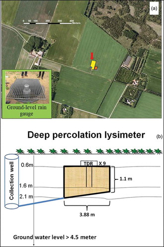
The study site was located at 56º2ʹ15.52′N and 9º9ʹ33.78′E, with an elevation of 62 m a.s.l., in the Skjern River catchment, western Jutland, Denmark. The hosting farm is a pig-breeding facility with 800 ha of cropland, including potatoes, rape seed, barley, maize and wheat. The investigated field (Fig. 1) represents the agricultural land use comprising approx. 68% of the Skjern River catchment. A 30-year meteorological record (1961–1990) indicates an average precipitation (P) of 781 mm/year with a mean annual temperature of 7.5ºC (Danish Meteorological Institute 2012). The soil is a cultivated Spodosol with 2% slope. The soil profile consists of Ap, Bhs, Bs, and C horizons extending to depths of 30, 50, 90 and 250 cm, respectively. The groundwater level at the site is typically below a depth of 4.5 m. The texture for the entire profile is sand (>90%), with a sparse gravel layer at a depth of 60 cm and a small increase in clay content (10% clay) at a depth of 1 m. The organic matter content is 0.3, 2.3, 1.2, 0.4 and 0.2% for soil depths of 10–20, 33–43, 61–71, 98–108 and 145–155 cm, respectively.

Fig. 1 Agricultural land-use field observations:. (a) locations of the fenced area of the agricultural field reserved for instrumentation (large, yellow rectangle), the eddy covariance flux tower (red arrow), the ground-level precipitation gauge (blue circle), and the four percolation lysimeters (small, orange rectangle); and (b) vertical cross-section of the lysimeter installation.

2.1.1 Study period

Field conditions over the 3.25 years investigated herein (October 2009–December 2012) included bare soil and crops, as shown on the cultivation sequence in Table 1. The periods to evaluate ET estimates from the lysimeter water balance and eddy covariance included both field conditions, as shown in Table 2, and the criteria used to define those periods is explained in Section 2.3. The lysimeter model calibration and validation periods (Table 3) do not include periods in which the lysimeter flow regime is not representative of the field situation due to redirection of snowmelt infiltration and, thus, snow accumulation and snowmelt were left out of this analysis. The heterogeneity in lysimeter D caused by meltwater diversion can be seen in the Appendix.

Table 1 Cultivation sequence.

Field condition	Bare  soil	Spring  barley	Bare  soil	Winter  barley	Bare  soil	Winter  Barley	Bare  soil	Winter  Rape
Begin	1 October 2009	1 April 2010	10 August 2010	13 September 2010	16 August 2011	15 September 2011	27/Jul//11	15 August 2012
End	1 April 2010	10 August 2010	13 September 2010	16 August 2011	15 September 2011	27 July 2011	15 August 2012	31 December 2012

Table 2 Periods for evaluation of evapotranspiration estimates from lysimeter water balance and eddy covariance.

Field condition	Period	Crop	Begin date	End date
Growing season	GS1	Spring barley	1 April 2010	9 August 2010
Bare soil and small winter crop	BS1	Winter barley 2011	10 August 2010	17 October 2010
Growing season	GS2	Winter barley 2011	30 March 2011	4 September 2011
Bare soil and small winter crop	BS2	Winter barley 2012	5 September 2011	31 October 2011
Growing season	GS3	Winter barley 2012	7 April 2012	7 September 2012
Bare soil and small winter crop	BS3	Winter rape 2013	8 September 2012	29 October 2012

Table 3 Periods for the lysimeter model calibration and validation.

Purpose	Field condition	Crop	Begin date	End date
Calibration	Bare soil	none	1 March 2010	30 March 2010
Calibration	Growing season	Spring barley	1 April 2010	31 July 2010
Calibration	Bare soil and small winter crop	Winter barley 2011	1 August 2010	30 September 2010
Validation	Small winter crop	Winter barley 2011	1 October 2010	30 November 2010
Validation	Growing season	Winter barley 2011	1 April 2011	31 July 2011
Validation	Bare soil and small winter crop	Winter barley 2012	1 August 2011	31 March 2012
Validation	Growing season	Winter barley 2012	1 April 2012	31 July 2012
Validation	Bare soil and small winter crop	Winter rape 2013	31 August 2012	24 December 2012

Irrigation was needed for 2010 and 2011: the 2010 spring barley crop was irrigated with 15, 25 and 25 mm on 4, 22 and 29 June, and the winter barley crop of 2011 was likewise irrigated with 20 mm on both 30 April and 23 May. No irrigation was needed in 2012, which was characterized by above average seasonal precipitation.

The instrumentation area within the agricultural field, as well as the location of the eddy covariance flux mast, lysimeter layout and ground-level precipitation gauge, are shown in Fig. 1 and described in detail below.

2.2 Field instrumentation

2.2.1 Lysimeter construction and observation well

The lysimeter facility (Fig. 1(b)) was constructed as part of the Hydrological Observatory (HOBE) initiative (Jensen and Illangasekare 2011) to improve the estimation of D and other water balance components.

Four percolation-lysimeters were installed during November 2008 following Benson et al. (2001), i.e. buried containers with open tops that collect and measure soil-water outflow (Fig. 1(b)). The area of each lysimeter is 3.2 m × 3.88 m and the depth varied from 1.1 to 1.5 m (Fig. 1(b)). The lysimeters were made from black polyethylene with welded seams, with a lower face of slope 10.3% along the 3.88-m side, inclining from 1.1 to 1.5 m depth (Fig. 1(b)). At the deep end (1.5 m), a permeable hose collects lysimeter discharge along the 3.2-m side. The sloping lower face was intended to facilitate discharge from the lysimeter and prevent the build-up of localized water tables at the lower boundary. The four lysimeters were located 30 cm apart. The lysimeters were buried with their upper face at a depth of 60 cm below the soil surface (Fig. 1(b)) to accommodate field operations with a ploughing depth of 30 cm. Lysimeter discharge was directed to a collection well placed 8.4 m west of the lysimeters. The collection well consisted of a rigid polyvinyl chloride (PVC) pipe section of 1.8 m diameter and 2.6 m length with access from the soil surface (Fig. 1(b)). The PVC pipes carried the lysimeter discharge to the observation well for measurement and collection of the water samples separately for each lysimeter. Water content in the lysimeters was measured with nine TDR probes in each lysimeter that were connected to a multiplexed TDR instrument placed inside the collection well. Details are given in Section 2.2.3.

The lysimeters were backfilled maintaining the order of the excavated soil horizons. After backfilling, nine 1-m-long balanced TDR probes were installed vertically from the upper face of each lysimeter. Finally, the lysimeters were covered with the original 60-cm surface soil preserving the original sequence of the two soil layers found in the upper 60 cm of soil (0–30 and 30–60 cm). Compaction of the sand material inside the lysimeters was made with hand-held wooden rammers of 20 cm × 20 cm and, for the upper soil, compaction and levelling was made with a small excavator. Soil bulk density was not sampled during the construction of the lysimeters, but considering the coarse sand material at the site, we did not expect to see any major effects of compaction at the time. Recording of water content and discharge started in June 2009, eight months after lysimeter installation.

2.2.2 Outflow measurements

Discharge was measured separately for each lysimeter with four VKWA 100 counters (UGT, Müncheberg, Germany) placed inside the observation well, each with a 100-mL polycarbonate tipping bucket including a 1% sub-sampling device. The number of tips was recorded and stored by a CR3000 data logger (Campbell Scientific Inc., UT, USA), which automatically transferred the last 24 hours of data to a server for data storage and access.

2.2.3 TDR system for measuring lysimeter water content

A self-contained TDR system, TC36, was developed for the HOBE lysimeter facility. The TC36 includes a compact PC unit, a TDR100 TDR instrument (Campbell Scientific Inc., UT, USA) and five eight-channel multiplexers, resulting in 36 available measurement channels. The system is housed in a 38 cm × 48 cm × 20 cm box. The TC36 software (Thomsen 1994) includes options for generating and testing multiprobe parameter sets and making automated measurements of soil moisture content. The software is similar to that developed by Baker and Allmaras (1990) and Heimovaara and Bouten (1990).

The 36 measurement probes installed in the lysimeters (nine in each lysimeter) are all of the balanced type including a custom-made (Trans Elektro A/S, Handsund, Denmark) balancing and impedance matching pulse transformer (Spaans and Baker 1993). The measuring depth of the probes extends vertically 1 m into the lysimeters from the upper face located at 60 cm below the soil surface (Fig. 1(b)). The TDR probes were made from 1-m-long stainless steel rods with a diameter of 6 mm, and separated by 5 cm. Water content was finally determined from the apparent dielectric permittivity of the soil using the Topp et al. (1980) calibration equation, which was shown to produce accurate water contents (RMSE ±1.5%) in a laboratory calibration (data not shown).

2.2.4 Eddy covariance measurements of water vapour fluxes

The eddy covariance instrumentation consisted of a sonic anemometer (R3-50, Gill Instruments Ltd., Lymington, UK) and an open path CO₂/ H₂O analyser (LI-7500, LI-COR, Lincoln, NE) mounted at a height of 6 m. The location of the EC measurements ensured that the fetch in major wind directions was not influenced by the instrumented area itself (Ringgaard et al. 2011). Typically, >80% of the time the measurement footprint was located within 50–500 m of the mast (Schuepp et al. 1990, Schelde et al. 2011). Data were measured at a frequency of 10 Hz. Raw EC data were processed using AltEddy software version 3.5 (Alterra, University of Wageningen, Wageningen, the Netherlands) and data gap filling followed the method adopted by CarboEurope and FLUXNET (Moffat et al. 2007). A detailed description of data processing and gap filling is given by Ringgaard et al. (2011).

2.2.5 Meteorological variables and soil heat flux

A four-component radiation sensor (NR01, Hukseflux Thermal Sensors BB, Delft, the Netherlands), and a temperature and humidity sensor (HMP 45 C, Vaisala Oyj, Helsinki, Finland) were mounted on the flux mast at a height of 4 m. Two soil heat flux plates (HFP01, Hukseflux Thermal Sensors) were buried 5 cm below the surface inside the field. The meteorological data were measured once every minute and the 10-min average stored in the data logger.

2.2.6 Precipitation

An international reference gauge (ground-level raingauge, Fig. 1) for the measurement of liquid precipitation was placed 20 m west of the lysimeters. It comprised a 200-cm² Pluvio2 (OTT Hach Environmental, Loveland, CO, USA) automatic raingauge. The gauge was placed in a pit covered by a metal grid with the opening at ground level and sufficient distance from the edges to avoid splash-in. The gauge was placed in the central opening of a metal anti-splash grid of 2 m × 2 m.

2.3 Variance of evapotranspiration estimate based on the mass balance residual of lysimeters

A simple statistical model for the variance of ETwb_Lys was used to generate uncertainty bounds on this estimate and facilitate comparison with the eddy covariance method. Assuming that distributions of the water balance components for the periods studied are known, or could be reasonably estimated with our experimental set-up of lysimeters, the model for the variance of ETwb_Lys is:

(1)

where var is the variance of each water balance component and cov is the covariance. Precipitation measured with the ground-level raingauge (Fig. 1(a)) was considered equal for the lysimeters during the growing seasons and after harvest; therefore, varP, cov(P,dS/dt) and cov(P RomD) were reduced to a value of zero.

Root zone water storage change, dS/dt_0–60 cm, defined as the difference between water stored at the beginning and the end of the growing season and late summer period was not measured above the lysimeters, but assumed to be the same as the difference in water content measured inside the lysimeters. This assumption is appropriate, as the start and end points (cut-off dates) for each period were chosen on the basis of identical boundary conditions, i.e. both start and end dates are characterized by a preceding 7-day period with little or no P (<3.5 mm) and small ET_REF (<2 mm d^-1), so that differences in root zone water storage were expected to be small at the cut-off dates. However, to further validate this assumption, we reviewed a reference dataset of non-replicated water content measurements in the root zone taken inside the fenced area in Fig. 1. The reference dataset documented that dS/dt_0–60cm for the periods shown in Table 2 was within 20 mm of the estimated lysimeter field root zone value. Therefore, ETwb_Lys and its variance estimate were mostly determined by the cumulative values of P and D and, to a smaller extent, to dS/dt in lysimeters and root zone for the periods analysed.

2.4 Lysimeter soil water flow model

The soil water flow model was set up in Hydrus 1D v 4.08 that numerically solves the Richards equation for variably saturated porous media (Šimůnek et al. 2008). Precipitation and reference Penman-Monteith evapotranspiration (Monteith 1981, Monteith and Unsworth 1990, FAO 1998), calculated from net radiation, air temperature, relative humidity and wind speed, were the atmospheric upper boundary fluxes used in modelling lysimeter water balance. However, soil evaporation switches from a prescribed reference flux (above) to a prescribed head boundary once a threshold pressure head (hCritA) is reached at the soil surface during simulation (Hydrus 1D Manual). The hCritA value is calculated from relative humidity and air temperature according to eq. 2.72 in the Hydrus 1D manual. Measurements of leaf area index (LAI) for the spring barley of 2010 (Jensen 2011) were used to partition reference ET into potential soil evaporation and transpiration following Beer’s law (Ritchie 1972). For the validation period including the winter barley of 2011 and 2012, LAI measurements were not available. Instead, LAI was estimated by linear interpolation of measurements of LAI made in the same field for the winter barley season of 2009, included in Ringgaard et al. (2011).

A normalized potential water uptake distribution over the root zone was considered following Hoffman and Van Genuchten (1983). The current rooting depth was estimated using a root growth coefficient following Šimůnek and Suarez (1993) and the maximum rooting depth was fixed at 60 cm based on field observations and Madsen (1985). Non-compensated root water uptake was modelled with a plant water stress response function proposed by Feddes et al. (1978). The barley crop water uptake model was assumed to be the same as Wesseling (1991) for wheat. A linear decrease in root water uptake with pressure head (Feddes et al. 1978) was modelled and transpiration reduced to 1.5 and 0.5 mm d^-1 for pressure head ranges of 500–900 and 900–16000 cm, respectively. Snow hydrology was modelled in a simplified form (Jarvis 1989), i.e. snow accumulates when air temperature ≤ −2ºC and precipitation is considered liquid when air temperature ≥2ºC. A linear transition was assumed between these two temperature thresholds. Also, snowmelt was modelled using a simple degree-day concept, where the snow layer melts proportionally to the air temperature whenever air temperature ≥ 0ºC by considering a snowmelt constant (Šimůnek et al. 2008).

The lower boundary condition in the lysimeters is a seepage face and the initial conditions of the soil profile were set to hydraulic equilibrium with zero pressure head at the bottom. The 1D soil column consisted of three soil materials, one each in the 0–25, 25–160 and 160–210 cm depths, respectively, and was based on observations of the effective plough layer (25 cm) made during a local excavation near the lysimeters in June 2010. Unsaturated soil hydraulic properties were represented by the model of Mualem (1976) for the hydraulic conductivity, in combination with a water retention function introduced by Vangenuchten (1980) given below:

(2)

(3)

and

(4)

where θ_r and θ_s are the residual and saturated water contents (mm³/mm³); α (1/mm) and n (-) are shape parameters for the soil hydraulic functions; K_s is saturated hydraulic conductivity (mm/d); S_e is relative saturation (-); and h is soil water matric potential.

To begin the model calibration, soil hydraulic parameters available in Hydrus 1D were assigned to the three soil materials (25 / 160 / 210 cm depth) based on soil texture (sand). Numerical problems arose and the hydraulic parameters of the topsoil (25 cm) were changed to loamy sand, sandy loam and loam soils, which allowed the numerical solution to be carried out. These three simulations were able to reproduce the eddy covariance ET (ET_EC), lysimeter drainage (D) and lysimeter water content (WC%) relatively well, based on the objective function:

(5)

where s_i² is the measurement variance, o_i the measurement average, and p_i the modelled value. Since there were no replicates for the eddy covariance flux measurements, an estimated ±10% uncertainty was considered, according to Herbst et al. (2011).

Agreement to the three datasets (EC, D and WC%) used for calibration was better with topsoil parameters set to sandy loam and loamy sand. These initial simulations were made keeping the hydraulic parameters for sand fixed for soil materials 2 and 3. Since the parameters for sandy loam topsoil offered the best approximation of the data, we defined those parameters as our starting point for optimization.

The pattern of lysimeter water content was well reproduced by the latter model realization, but its magnitude was not. Therefore, to scale the lysimeter water content, the θ_r parameter for soil material 2 (25–160 cm) was increased from 0.045 to 0.11, which was in agreement with the magnitude of lysimeter water contents observed. Adjusting θ_r was justified at this depth (0.25–1.6 m) due to a small clay content increase (10% clay) found at a depth of 1 m in this otherwise very sandy soil.

In a further step, the parameter α from the top soil was iteratively calibrated with the EC and D data on the parameter range of 0.075–0.124 cm^-1, which represents the parameter value for a sandy loam and a loamy sand in the Hydrus 1D database. The α parameter was chosen for optimization since it is one of the soil hydraulic parameters that is most difficult to identify with pedotransfer functions (together with K_s) and thus was optimized against field observations (Pollacco et al. 2008). The optimized α value for the top soil was 0.085 cm^-1.

Next, parameters α and K_s for the soil materials 2 and 3 (25–160 and 160-210 cm) were optimized using the Marquardt-Levenberg type algorithm available in Hydrus 1D, with parameter ranges of 0.01–0.2 cm^-1 and 250–1000 cm d^-1, respectively. Furthermore, different initial values of α and K_s parameters were tested (nine different combinations) to reduce the risk of finding local minima. The results of the nine different optimization runs allowed us to choose the parameters with the least sum of normalized squared residuals for EC, D and WC%, according to equation (5).

2.4.1 Model goodness-of-fit indicators

To introduce measurement uncertainty in the evaluation of model predictive ability, the correction factor (CF) of Harmel and Smith (2007) and Harmel et al. (2010) was applied to the residuals (observed – predicted). The CF is the probability to find model deviations between the observed and predicted values and, thus, larger deviations (residuals) translate into larger CFs. The CF was obtained assuming a one-tailed standard normal distribution with mean and median equal to the observed value (measurement average) and the variance equal to the measurement variance. Next, the CF value was divided by 0.5, which is the maximum probability for one-sided probability distributions, to represent the proportion of the deviation (0–1) (Harmel and Smith 2007). In summary, good model performance was assumed for the case of small residuals and thus small CFs for modelled values within ±1 standard deviations (SD) of the measurements. For modelled values larger than ±1 SD, CF was set to 1 and, thus, no correction was considered.

3 RESULTS AND DISCUSSION

3.1 Variability in deep percolation

The variability in storage measurements within lysimeters (±13 mm) was smaller than that between lysimeters (±22 mm), as seen in Fig. 2, indicating that our experimental set-up was adequate to describe the heterogeneity in lysimeter storage that was within the ±2% volumetric water content accuracy expected for TDR measurements (Jones et al. 2002).

Fig. 2 (a) Drainage measured 2.1 m below soil surface with four buried zero-tension lysimeters in a spring barley field. (b)–(e) Evolution of water storage below the root zone of lysimeters measured with nine vertical TDR profiles at different positions within each lysimeter.

Lysimeter D measured on the first recharge period after harvest (15 August–7 September 2010) is shown in Fig. 2: values ranged from 90 to 136 mm, with a coefficient of variation of ±18%, which was attributed to differences in hydraulic properties of repacked lysimeters. This heterogeneity in hydraulic properties may result from water repellence in the Bh horizon causing finger-like flow and thus different responses in lysimeter D. Finger-like flow processes have been identified at the site using dye tracer experiments (Haarder et al. 2011) and are most likely involved in water flow diversion not caused by redirection of snowmelt infiltration. Moreover, large increases in S were observed for lysimeters 1 and 4, which supported the larger cumulative D observed in these lysimeters (Fig. 2).

The variability in annual D (Table 4) increased with the occurrence and accumulation of solid precipitation in winter from ±6% in a year without snow (October 2011–September 2012) to ±14% in a year with ample snow accumulation (2009/10). Estimates of D for winters dominated by solid precipitation should be taken with caution, since redirection of snowmelt infiltration due to frozen topsoil, as was observed in the area, may render D estimates not representative of the field conditions.

Table 4 Water balance for the agricultural field site in Skjern River catchment including model calibration, validation and comparison of evapotranspiration estimates with their variability.

Hydrological years	Precipitation	Evapotranspiration			Drainage
		Measured	Modelled	ETwbLys	Measured	Modelled
Oct. 2009–Sep. 2010	923	416 ± 42	415		537 ± 75	513
Oct. 2010–Sep. 2011	1102	401 ± 40	470		605 ± 61	611
Oct. 2011–Sep. 2012	1092	465 ± 47	466		612 ± 36	574
Model calibration
1–31 Mar. 2010	27	25 ± 3	10		20 ± 8	12
1 Apr.–31 Jul. 2010	318	286 ± 29	287		73 ± 8	50
1 Aug.–30 Sep. 2010	280	82 ± 8	102		167 ± 27	170
Model validation
1 Oct.–30 Nov. 2010	201	28 ± 3	28		197 ± 17	162
1 Apr.–31 Jul. 2011	300	251 ± 25	279		60 ± 9	33
1 Aug. 2011–31 Mar. 2012	863	180 ± 18	217		620 ± 37	634
1 Apr.–31 Jul. 2012	310	274 ± 7	266		74 ± 3	32
1 Aug.–24 Dec. 2012	469	139 ± 14	128		392 ± 17	328
Evapotranspiration estimates
GS1: 1 Apr.–9 Aug. 2010	324	298 ± 30	305	278 ± 13	75 ± 8	52
BS1: 10 Aug.–17 Oct. 2010	287	84 ± 8	100	91 ± 23	178 ± 24	185
GS2: 30 Mar.–4 Sep. 2011	438	301 ± 30	353	289 ± 12	141 ± 12	56
BS2: 5 Sep.–31 Oct. 2011	288	61 ± 6	68	79 ± 12	209 ± 12	215
GS3: 7 Apr.–7 Sep. 2012	396	335 ± 34	326	269 ± 4	122 ± 4	45
BS3: 8 Sep.–29 Oct. 2012	258	59 ± 6	47	21 ± 10	221 ± 10	182

*All units in mm

In summary, most of the differences among lysimeter D occurred during periods with redirection of snowmelt infiltration (see Appendix), or when high precipitation intensity coincided with relatively wet soils (August 2010), as seen in Figs 2 and 3. For the case of meltwater diversion due to frozen top soils, the net result was an overestimation of D due to a larger contributing area during snowmelt infiltration. For the case of high-intensity rainfall coinciding with initially wet soils, differences in D were attributed to heterogeneity in hydraulic properties of repacked lysimeters that were most likely related to finger-like flow processes causing dynamic effects on water flow (Diamantopoulos and Durner 2012).

3.2 Evaluating ETwb_Lys against ET_EC

The purpose of this comparison was to evaluate two independent measurement techniques. Therefore, accumulated values of ETwb_Lys were chosen on the basis of small differences in lysimeter S between the start and end points for each period considered, as shown in Fig. 4 and Table 2. The change in modelled root zone water storage and measured lysimeter S for the periods chosen to evaluate ET estimates (Table 2) can be seen in Figs 3(b) and (c) and 5(b) and (c). The inferred change in root zone water storage (assuming comparable water contents in lysimeters and in the root zone at cut-off dates) were −9.6, +4.6, +2, +0.13, +2.4 and +5.8 mm, and were in reasonable agreement with modelled root zone storage changes of −25, −0.06, +10, −4.9, +12.7 and +22.4 mm for each of the periods evaluated in Fig. 4. The small changes in modelled root zone storage further supported our assumption of comparable water contents in lysimeters and root zone for the cut-off dates defined in Table 2. These cut-off dates were characterized by a precedent 7-day period with low rainfall (<3.5 mm. d^-1) and small ET_REF (<2 mm d^-1) and thus contributed to minimize the impact of root zone storage changes in our lysimeter water balance estimate of ET. This approach was intended since lysimeter root zone water content was not measured.

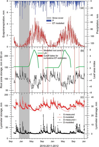
Fig. 3 Daily measurements and modelled water balance components in a spring barley field located in the Skjern River catchment. Shaded areas indicate periods with snow cover. (a) Measured and modelled evapotranspiration, (b) modelled root zone water storage and leaf area index, and (c) measured and modelled lysimeter storage and drainage.

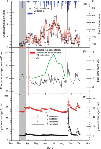
Fig. 4 Evapotranspiration estimates for the agricultural field observatory in Skjern River catchment. Comparison of eddy covariance flux measurements, ET_EC, against the mass balance residual of four buried zero-tension lysimeters, ETwb_Lys. Field conditions studied include periods with bare soil surface and small winter crop (BS) and the active growing season (GS) during three years (2010–2012).

Due to the measurement problems with redirection of snowmelt infiltration, only the periods when lysimeters were not influenced by snow accumulation and snowmelt were used for the comparison of ET estimates below.

Good agreement between ETwb_Lys and ET_EC was found for the growing seasons of 2010 and 2011 (GS1 and GS2), but not for 2012 (GS3), with a difference of 20, 12 and 66 mm, representing 7, 4 and 20% of measured ET_EC, respectively (Fig. 4). The EC-measured latent heat and sensible heat accounted for 74, 73 and 83% of measured net radiation and ground heat flux for the three growing seasons, and the larger difference in ET estimates for GS3 was attributed to increased soil evaporation originating from autumn surface soil treatment, which was included in GS3 but not in GS1 and GS2. The larger ET_EC for GS3 may have resulted from exposing a moist soil layer to the surface during soil turn-over.

Correcting ET_EC for lack of surface energy balance closure during the growing seasons would further increase the difference relative to ETwb_Lys by an order of magnitude as shown in Fig. 4. This is in agreement with findings by Scott (2010), who compared 13 years of ET from small semi-arid watersheds obtained by water balance modelling (ET_WB) against ET_EC and found that both independent techniques agreed within an average of 3% annually. Best agreements were found for dry years and at topographically less complex sites. Furthermore, forcing energy balance closure on ET was not recommended because it led to large discrepancies for nine out of the 13 years included in the study of Scott (2010).

Wilson et al. (2001) also found good agreement between annual estimates of ET_EC and catchment water balance for a mixed deciduous forest catchment. Annual average ET for the two methods agreed within 12 mm for a 5-year period despite the lack of energy balance closure (80%). The ET_EC in Wilson et al. (2001) correlated well with a soil water budget estimate from soil moisture measurements. However, high spatial variability of the soil moisture profile, and uncertainties concerning drainage and rooting depths caused a large scatter around this correlation, resulting in an approximately 60% lower ET estimate based on soil moisture compared to ET_EC (Wilson et al. 2001). A more recent comparison between ET_EC and soil moisture depletion (SMD) from the root zone at the current study site (Schelde et al. 2011) suggested that SMD measured during dry periods where zero flux at the lower boundary is assumed could serve as a lower limit confinement for ET_EC. In their study, daily differences between ET_EC and SMD agreed within 1 mm for four dry periods (2–5 days) during the growing season, with ET_EC, on average, 10% higher ET than SMD. Better agreement between SMD and ET_EC in Schelde et al. (2011) is probably due to better defined upper and lower boundary conditions for the dry periods studied. However, different gas analysers were used in Schelde et al. (2011) (Closed path Li-7000) and in our study (Open path LI-7500) to obtain ET_EC. This is important because tube attenuation in the closed path sensor may lead to underestimation of ET_EC.

The general good agreement observed between ETwb_Lys and ET_EC during the growing seasons of 2010 and 2011 was consistent with small water fluxes at the lower boundary in the lysimeters (Fig. 3(c)) that resulted in a small SD of ±13 and ±12 mm for the estimated ETwb_Lys (Fig. 4). Although we found that correcting ET_EC for lack of energy balance closure will lead to larger discrepancies against ETwb_Lys for all the growing seasons, it was not possible to define whether this correction is appropriate, since our estimate of uncertainty for ET_EC (±10%) was two to eight times larger than that of ETwb_Lys (Table 4). For the periods with bare soil surface and a small winter crop (BS1–BS3), the agreement between ET_EC and ETwb_Lys was not affected by the lack of energy balance closure, as latent and sensible heat flux accounted for 0.98, 0.96 and 0.75 of the available net radiation and ground heat flux. The smaller ETwb_Lys for BS3 in Fig. 4 appeared to originate from a slightly larger D for that period, which was not consistent with an increase in precipitation (Table 4). A 2-day rainfall event of 130 mm in August 2012 (Fig. 3(a)) increased the variability in measured D, which resulted in a large SD of ±23 mm for ETwb_Lys during BS1 compared to half of that for BS2 and BS3(Table 4). Because the uncertainty in ETwb_Lys was three times larger than that of ET_EC during BS1 (Table 4), it was not possible to define whether the correction for lack of surface energy balance was appropriate.

In summary, ET_EC in our study was in good agreement with ETwb_Lys for the growing seasons and periods with bare soil surface and small winter crops which supports similar comparisons where catchment water balance and SMD have been used to validate ET_EC. However, due to the uncertainties involved in each of the methods compared, it was not possible to define whether a correction for lack of surface energy balance closure in ET_EC was appropriate.

3.3 Application of the lysimeter soil water flow model

Table 5 presents the optimized MVG soil hydraulic parameters used in modelling lysimeter water flow. We adopted a ±10% uncertainty for ET_EC measurements, as suggested by Herbst et al. (2011), to calculate correction factors for goodness-of-fit indicators (see Section 2.4.1).

Table 5 Optimized soil hydraulic property parameters for Mualem-van Genuchten model used to simulate water flow in lysimeters repacked with sandy soil.

Depth (cm)	θr	θs	α (cm^-1)	n	Ksat (cm d^-1)	l
25	0.065	0.41	0.085*	1.89	106	0.5
160	0.11*	0.43	0.2*	2.68	840*	0.5
210	0.045	0.43	0.08108*	2.68	993*	0.5

*Fitted parameters

Modelled ET described ET_EC with a mean absolute error (MAE) of 0.5 mm d^-1 for the growing season of 2010 (Table 6); however, most of the model error occurred in the months of April and May 2010, with LAI < 1 suggesting that, for field conditions with bare soil or a small crop, our simple model failed to reproduce the complex dynamics of soil evaporation. The complexities of the soil hydraulic functions at the dry end that are likely to occur at or near the soil surface were not considered in our recharge model and could affect soil evaporation. For instance, Peters (2013) found that neglecting adsorptive water retention and film conductivity in the dry range can lead to a significant underestimation of water transport at low water contents. Furthermore, soil evaporation may be complicated by partial wettability phenomena affecting water retention and flow stability (Or et al. 2013), which are particularly important in Podzolic soils like the one investigated here. For the growing season with LAI > 1 (1 June–31 July 2010), modelled ET was in reasonable agreement with ET_EC, with a MAE of 0.33 mm d^-1, although modelled ET underestimated ET_EC from 10 to 18 April 2010, due to underestimation of the snowmelt input associated with uncertainties in solid precipitation.

Table 6 Goodness-of-fit indicators for the soil water flow model following Harmel and Smith (2007) for calibration and validation periods.

	Calibration			Validation
	1–31 Mar.	1 Apr.–31 Jul.	1 Aug.–30 Sep.	1 Oct.–30 Nov.	1 Apr.–31 Jul.	1 Aug.–31 Mar.	1 Apr.–31 Jul.	1 Aug.–24 Dec.
Year	2010	2010	2010	2010	2011	2011/12	2012	2012
Field conditions	Bare soil	Growing season	Bare soil + winter crop	Bare soil + winter crop	Growing season	Bare soil + winter crop	Growing season	Bare soil + winter crop
ET (mm)
RMSE	0.3	0.66	0.64	0.22	0.86	0.53	0.82	0.5
MAE	0.23	0.5	0.46	0.16	0.66	0.37	0.61	0.35
C. efficiency	0.17	0.51	0.12	0.43	0.14	0.24	0.23	0.46
I. Agreement	0.6	0.78	0.62	0.56	0.48	0.53	0.44	0.53
Storage (mm)
RMSE	6.4	6.2	8.7	8.4	9.5	9.0	12.6	10.5
MAE	3.1	3.3	4.9	4.8	6.4	5.5	10.9	7.2
C. efficiency	0.59	0.25	0.47	0.42	−0.005	0.1	−1.31	−0.12
I. Agreement	0.78	0.71	0.79	0.61	−0.35	0.47	−0.17	0.32
Drainage (mm d^−1)
RMSE	0.7	0.36	4.4	2.95	0.52	3.2	0.7	2.4
MAE	0.44	0.27	2	1.52	0.33	1.7	0.4	1.4
C. efficiency	0.31	−0.16	0.23	0.34	0.01	0.06	−0.14	0.25
I. Agreement	0.6	0.53	0.64	0.16	−0.35	0.2	−0.1	0.31

Good agreement between measured and modelled lysimeter water storage (S) is shown in Fig. 3(c) for the entire growing season (calibration period), with a RMSE of 6.2 mm, a coefficient of efficiency (CoE) of 0.25 and an index of agreement (IoA) of 0.71 (Table 6). This good agreement was probably due to the nature of the infiltration process during the growing season, with small changes in lysimeter S and D events indicating that most of the available water in the root zone was taken up by the crop.

At our study site, the recharge process was concentrated during late summer and autumn (August–December) and winter (January–March) when most of the precipitation occurred and reference ET is small. The seasonality of the recharge process showed a dynamic behaviour of lysimeter S and D during autumn and winter contrasting with that of the growing season (April–July, Figs 3 and 5). Therefore, higher MAE and RMSE with lower CoE and IoA (Table 6) was expected for periods where lysimeter S and D were highly dynamic. Modelled D had a RMSE of +4.4 mm d^-1 during calibration period (August and September 2010) and decreased during validation to +3 mm d^-1 for similar periods with large D events in Table 6. Our simple model calibration approach failed to reproduce the small but steady D for the growing season of 2010 in Table 6, where a negative CoE indicates that the measured average D was a better estimate than our modelled D. Agreement between measured and modelled D increased during the validation period, as indicated by a decrease in MAE and RMSE in Table 6. In general, fair agreement between measured and modelled lysimeter ET, S and D was found for both calibration and validation periods (Table 6). Our simple modelling approach does not allow for a full exploration of the parameter space and, thus, the possibility that a better set of soil hydraulic parameters exists to describe our data remains open.

Fig. 5 Validation period for the lysimeter water flow model: (a) precipitation and modelled evapotranspiration; (b) modelled root zone storage, leaf area index and cut-off dates for comparison of ET estimates; and (c) measured and modelled lysimeter storage and drainage.

However, the degree to which key modelling assumptions are met in our Podzol may also affect the predictive ability of our model. For instance, it is well documented that sandy Podzols often exhibit water repellence in the Bh horizon leading to an unstable wetting and infiltration front and possibly funnelled flow (Kung 1990, Or et al. 2013), which violates our assumption of vertical slow and one-dimensional water flow. Also, surface soil treatment may change the top soil hydraulic properties temporarily due to tillage operations and could result in dynamic non-equilibrium effects on water flow (Diamantopoulos and Durner 2012). This has been previously observed by Wildenschild et al. (2001), who found an infiltration rate dependence on soil hydraulic characteristics for sandy soils with a general tendency of increasing hydraulic conductivity as flow rate increased. The authors attributed these findings to water entrapment, pore blockage and discontinuity of the air phase during high flow rates which caused a significant deviation from static equilibrium. Despite all the difficulties associated with our modelling approach and the systematic errors in D due to meltwater diversion, annual D was in reasonable agreement with measured D for the 3 years of this study (Table 4).

Moreover, modelled D was within ±75, ±61 and ±36 mm, or one SD of the measured D, in lysimeters for the three years summarized in Table 4, suggesting an overall acceptable model performance, given the uncertainty in measured D.

In summary, measured D for the calendar years of 2010, 2011 and 2012 was 537, 562 and 704 mm, with modelled D of 486, 624 and 613 mm, respectively. Most of the differences between measured and modelled D were caused by a systematic bias of drainage measurements, due to redirection of snowmelt infiltration and temporal changes in near surface effective hydraulic properties caused by surface soil treatment possibly leading to dynamic non-equilibrium (Diamantopoulos and Durner 2012).

4 CONCLUSIONS

Good agreement was found between ETwb_Lys and ET_EC despite their different measurement techniques, footprint area, and the lack of energy balance closure for ET_EC. It was not possible to define whether a correction for lack of surface energy balance closure in ET_EC was appropriate because of relatively large uncertainties in ETwb_Lys and ET_EC. Good agreement between independent measurements of ET suggests that lysimeters were sufficiently large to capture a significant part of the field-scale variability in soil water balance at the site.

Larger lysimeter S and D variability was observed during snowmelt when frozen topsoils may have redirected infiltration. However, for periods without meltwater diversion, larger measurement variability was found in D than in S, and was attributed to heterogeneity between repacked lysimeters.

The soil water flow model was able to reproduce the dynamics of the water balance components adequately. A more sophisticated evaporation model accounting for the two stages of soil evaporation combined with a more flexible model structure using free formed functions, like the one proposed by Bitterlich et al. (2004) and Iden and Durner (2007) may improve the overall model performance and allow for a better representation of the measured ET, S and D.

Disclosure statement

No potential conflict of interest was reported by the author(s).

Acknowledgements

The authors would like to thank Wolfgang Durner and an anonymous referee for their constructive comments on an earlier version of this paper.

Additional information

Funding

This study is part of HOBE Hydrological Observatory, a VKR Centre of excellence funded by the Villum Foundation.

Appendix

Fig. A1 Heterogeneity in lysimeter drainage caused by redirection of snowmelt infiltration.

REFERENCES

- Allen, R.G., et al., 2011. Evapotranspiration information reporting: I. Factors governing measurement accuracy. Agricultural Water Management, 98 (6), 899–920. doi:10.1016/j.agwat.2010.12.015
- Baker, J.M. and Allmaras, R.R., 1990. System for automating and multiplexing soil-moisture measurement by time-domain reflectometry. Soil Science Society of America Journal, 54 (1), 1–6. doi:10.2136/sssaj1990.03615995005400010001x
- Baldocchi, D., et al., 2001. FLUXNET: A new tool to study the temporal and spatial variability of ecosystem-scale carbon dioxide, water vapor, and energy flux densities. Bulletin of the American Meteorological Society, 82 (11), 2415–2434. doi:10.1175/1520-0477(2001)082<2415:FANTTS>2.3.CO;2
- Benson, C., et al., 2001. Field evaluation of alternative earthen final covers. International Journal of Phytoremediation, 3, 105–127. doi:10.1080/15226510108500052
- Bitterlich, S., et al., 2004. Inverse estimation of the unsaturated soil hydraulic properties from column outflow experiments using free-form parameterizations. Vadose Zone Journal, 3 (3), 971–981. doi:10.2136/vzj2004.0971
- Burba, G.G., et al., 2010. Novel design of an enclosed CO2/H2O gas analyser for eddy covariance flux measurements. Tellus Series B—Chemical and Physical Meteorology, 62 (5), 743–748. doi:10.1111/j.1600-0889.2010.00468.x
- Castellví, F. and Snyder, R.L., 2010. A comparison between latent heat fluxes over grass using a weighing lysimeter and surface renewal analysis. Journal of Hydrology, 381 (3–4), 213–220. doi:10.1016/j.jhydrol.2009.11.043
- Chávez, J.L., Howell, T.A., and Copeland, K.S., 2009. Evaluating eddy covariance cotton ET measurements in an advective environment with large weighing lysimeters. Irrigation Science, 28 (1), 35–50. doi:10.1007/s00271-009-0179-7
- Danish Meteorological Institute. 2012. Published weather database for Denmark [online]. Danish Meteorological Institute, Copenhagen, Denmark. Available from: http://www.dmi.dk/dmi/index/danmark/klimanormaler.htm [Accessed 27 July 2012].
- Diamantopoulos, E. and Durner, W., 2012. Dynamic nonequilibrium of water flow in porous media: a review. Vadose Zone Journal, 11, 3. doi:10.2136/vzj2011.0197
- Evett, S.R., et al., 2012. Can weighing lysimeter ET represent surrounding field ET well enough to test flux station measurements of daily and sub-daily ET? Advances in Water Resources, 50, 79–90.
- Feddes, R.A., Kowalik, P.J., and Zaradny, H., 1978. Simulation of field water use and crop yield. New York: John Wiley and Sons.
- FAO (Food and Agriculture Organization), 1998. Crop evapotranspiration: guidelines for computing crop requirements [online]. Rome, Italy: Food and Agriculture Organization. Available from: http://www.fao.org/docrep/X0490E/X0490E00.htm [Accessed 10 February 2012].
- Gee, G.W., et al., 2002. A vadose zone water fluxmeter with divergence control. Water Resources Research, 38 (8), 16-1–16-7. doi:10.1029/2001WR000816
- Haarder, E.B., et al., 2011. Visualizing unsaturated flow phenomena using high-resolution reflection ground penetrating radar. Vadose Zone Journal, 10 (1), 84–97. doi:10.2136/vzj2009.0188
- Harmel, R.D. and Smith, P.K., 2007. Consideration of measurement uncertainty in the evaluation of goodness-of-fit in hydrologic and water quality modeling. Journal of Hydrology, 337 (3–4), 326–336. doi:10.1016/j.jhydrol.2007.01.043
- Harmel, R.D., Smith, P.K., and Migliaccio, K.W., 2010. Modifying goodness-of-fit indicators to incorporate both measurement and model uncertainty in model calibration and validation. Transactions of the ASABE, 53 (1), 55–63. doi:10.13031/2013.29502
- Heimovaara, T.J. and Bouten, W., 1990. A computer-controlled 36-channel time domain reflectometry system for monitoring soil-water contents. Water Resources Research, 26 (10), 2311–2316.
- Herbst, M., et al., 2011. Catchment-wide atmospheric greenhouse gas exchange as influenced by land use diversity. Vadose Zone Journal, 10 (1), 67–77. doi:10.2136/vzj2010.0058
- Hoffman, G.J. and Van Genuchten, M.T., 1983. Soil properties and efficient water use: water management for salinity control. In: H.M. Taylor, W.R. Jordan, and T.R. Sinclair, ed. Limitations and efficient water use in crop production. Madison, WI: American Society of Agronomy, 73–85
- Iden, S.C. and Durner, W., 2007. Free-form estimation of the unsaturated soil hydraulic properties by inverse modeling using global optimization. Water Resources Research, 43, 7. doi:10.1029/2006WR005845
- Jarvis, N.J., 1989. A simple empirical-model of root water-uptake. Journal of Hydrology, 107 (1–4), 57–72. doi:10.1016/0022-1694(89)90050-4
- Jensen, K.H. and Illangasekare, T.H., 2011. HOBE: A hydrological observatory. Vadose Zone Journal, 10 (1), 1–7. doi:10.2136/vzj2011.0006
- Jensen, R., 2011. Measured and modelled exchange of carbon dioxide from a Danish agricultural site—application of a “big-leaf” model to estimate flux partitioning. Thesis (MSc). University of Copenhagen.
- Jones, S.B., Wraith, J.M., and Or, D., 2002. Time domain reflectometry measurement principles and applications. Hydrological Processes, 16 (1), 141–153. doi:10.1002/hyp.513
- Kung, K.-J.S., 1990. Preferential flow in a sandy vadose zone: 2. Mechanism and implications. Geoderma, 46 (1–3), 59–71. doi:10.1016/0016-7061(90)90007-V
- Madsen, H.B., 1985. Distribution of spring barley roots in Danish soils of different texture and under different climatic conditions. Plant and Soil, 88 (1), 31–43. doi:10.1007/BF02140664
- Moffat, A.M., et al., 2007. Comprehensive comparison of gap-filling techniques for eddy covariance net carbon fluxes. Agricultural and Forest Meteorology, 147 (3–4), 209–232. doi:10.1016/j.agrformet.2007.08.011
- Monteith, J.L., 1981. Evaporation and surface-temperature. Quarterly Journal of the Royal Meteorological Society, 107 (451), 1–27. doi:10.1002/qj.49710745102
- Monteith, J.L. and Unsworth, M.H., 1990. Principles of environmental physics. 2nd ed. London: Hodder and Stoughton.
- Mualem, Y., 1976. A new model for predicting the hydraulic conductivity of unsaturated porous-media. Water Resources Research, 12 (3), 513–522. doi:10.1029/WR012i003p00513
- Or, D., et al., 2013. Advances in soil evaporation physics-A review. Vadose Zone Journal, 12, 4. doi:10.2136/vzj2012.0163
- Peters, A., 2013. Simple consistent models for water retention and hydraulic conductivity in the complete moisture range. Water Resources Research, 49 (10), 6765–6780. doi:10.1002/wrcr.20548
- Pollacco, J.A.P., et al., 2008. A Linking Test to reduce the number of hydraulic parameters necessary to simulate groundwater recharge in unsaturated soils. Advances in Water Resources, 31 (2), 355–369. doi:10.1016/j.advwatres.2007.09.002
- Ringgaard, R., et al., 2011. Energy fluxes above three disparate surfaces in a temperate mesoscale coastal catchment. Vadose Zone Journal, 10 (1), 54–66. doi:10.2136/vzj2009.0181
- Ritchie, J.T., 1972. Model for predicting evaporation from a row crop with incomplete cover. Water Resources Research, 8 (5), 1204–1213. doi:10.1029/WR008i005p01204
- Scanlon, B.R., Healy, R.W., and Cook, P.G., 2002. Choosing appropriate techniques for quantifying groundwater recharge. Hydrogeology Journal, 10 (1), 18–39. doi:10.1007/s10040-001-0176-2
- Schelde, K., et al., 2011. Comparing evapotranspiration rates estimated from atmospheric flux and TDR soil moisture measurements. Vadose Zone Journal, 10 (1), 78–83. doi:10.2136/vzj2010.0060
- Schuepp, P.H., et al., 1990. Footprint prediction of scalar fluxes from analytical solutions of the diffusion equation. Boundary-Layer Meteorology, 50 (1–4), 355–373. doi:10.1007/BF00120530
- Scott, R.L., 2010. Using watershed water balance to evaluate the accuracy of eddy covariance evaporation measurements for three semiarid ecosystems. Agricultural and Forest Meteorology, 150 (2), 219–225. doi:10.1016/j.agrformet.2009.11.002
- Šimůnek, J. and Suarez, D.L., 1993. Modeling of carbon dioxide transport and production in soil: 1. Model development. Water Resources Research, 29 (2), 487–497. doi:10.1029/92WR02225
- Šimůnek, J., Van Genuchten, M.T., and Šejna, M., 2008. Development and applications of the HYDRUS and STANMOD software packages and related codes. Vadose Zone Journal, 7 (2), 587–600. doi:10.2136/vzj2007.0077
- Sophocleous, M.A., 1991. Combining the soilwater balance and water-level fluctuation methods to estimate natural groundwater recharge: practical aspects. Journal of Hydrology, 124 (3–4), 229–241. doi:10.1016/0022-1694(91)90016-B
- Spaans, E.J.A. and Baker, J.M., 1993. Simple baluns in parallel probes for time domain reflectometry. Soil Science Society of America Journal, 57, 668–673. doi:10.2136/sssaj1993.03615995005700030006x
- Thomsen, A. 1994. Program AutoTDR for making automated TDR measurements of soil water content. Aarhus: Faculty of Agricultural Sciences, Aarhus University, Special Report 38.
- Thomsen, A., et al., 2007. Mobile TDR for geo-referenced measurement of soil water content and electrical conductivity. Precision Agriculture, 8 (4–5), 213–223. doi:10.1007/s11119-007-9041-1
- Topp, G.C., Davis, J.L., and Annan, A.P., 1980. Electromagnetic determination of soil water content: measurements in coaxial transmission lines. Water Resources Research, 16 (3), 574–582. doi:10.1029/WR016i003p00574
- Vangenuchten, M.T., 1980. A closed-form equation for predicting the hydraulic conductivity of unsaturated soils. Soil Science Society of America Journal, 44 (5), 892–898. doi:10.2136/sssaj1980.03615995004400050002x
- Wesseling, J.G. 1991. CAPSEV: steady state moisture flow theory, program description and user manual. Wageningen, The Netherlands: Winand Staring Centre, Report 37.
- Western, A.W., Grayson, R.B., and Blöschl, G., 2002. Scaling of soil moisture: a hydrologic perspective. Annual Review of Earth and Planetary Sciences, 30, 149–180. doi:10.1146/annurev.earth.30.091201.140434
- Wildenschild, D., Hopmans, J.W., and Simunek, J., 2001. Flow rate dependence of soil hydraulic characteristics. Soil Science Society of America Journal, 65 (1), 35–48. doi:10.2136/sssaj2001.65135x
- Wilson, K., et al., 2002. Energy balance closure at FLUXNET sites. Agricultural and Forest Meteorology, 113 (1–4), 223–243. doi:10.1016/S0168-1923(02)00109-0
- Wilson, K.B., et al., 2001. A comparison of methods for determining forest evapotranspiration and its components: sap-flow, soil water budget, eddy covariance and catchment water balance. Agricultural and Forest Meteorology, 106 (2), 153–168. doi:10.1016/S0168-1923(00)00199-4
- Wohlfahrt, G. and Widmoser, P., 2013. Can an energy balance model provide additional constraints on how to close the energy imbalance? Agricultural and Forest Meteorology, 169, 85–91. doi:10.1016/j.agrformet.2012.10.006