Assessment of sediment transport approaches for sand-bed rivers by means of machine learning

Abstract

The quantification of the sediment carrying capacity of a river is a difficult task that has received much attention. For sand-bed rivers especially, several sediment transport functions have appeared in the literature based on various concepts and approaches; however, since they present a significant discrepancy in their results, none of them has become universally accepted. This paper employs three machine learning techniques, namely artificial neural networks, symbolic regression based on genetic programming and an adaptive-network-based fuzzy inference system, for the derivation of sediment transport formulae for sand-bed rivers from field and laboratory flume data. For the determination of the input parameters, some of the most prominent fundamental approaches that govern the phenomenon, such as shear stress, stream power and unit stream power, are utilized and a comparison of their efficacy is provided. The results obtained from the machine learning techniques are superior to those of the commonly-used sediment transport formulae and it is shown that each of the input combinations tested has its own merit, as they produce similarly good results with respect to the data-driven technique employed.

Editor Z.W. Kundzewicz

Résumé

La quantification de la capacité de transport de sédiments d’une rivière est une tâche difficile, qui a reçu beaucoup d’attention. Pour les rivières à lit sableux en particulier, plusieurs fonctions de transport des sédiments ont été publiées dans la littérature sur la base de divers concepts et approches; cependant, comme leurs résultats sont significativement différents, aucune d’entre elles n’est aujourd’hui universellement acceptée. Cet article utilise trois techniques d’apprentissage automatique pour l’estimation de formules de transport de sédiments dans les rivières à lit sableux à partir des données de terrain et de canal de laboratoire, à savoir les réseaux de neurones artificiels, la régression symbolique basée sur la programmation génétique, et un système d’inférence floue basé sur un réseau adaptatif. Pour la détermination des paramètres d’entrée, certaines des plus importantes approches fondamentales régissant le phénomène, telles que la contrainte de cisaillement, la puissance du courant et la puissance unitaire du courant, ont été utilisées, et une comparaison de leur efficacité a été réalisée. Les résultats obtenus à partir des techniques d’apprentissage automatique sont meilleurs que ceux des formules de transport de sédiments couramment utilisées et nous avons pu montrer que chacune des approches d’apprentissage automatique a ses mérites propres, car elles produisent des résultats aussi bons par rapport à la technique orientée données employée.

Key words:

• adaptive-network-based fuzzy inference system
• artificial neural networks
• genetic programming
• machine learning
• sand-bed rivers
• sediment transport

Mots clefs:

• système d’inférence floue basé sur un réseau adaptatif
• réseaux de neurones artificiels
• programmation génétique
• apprentissage automatique
• rivières à lit sableux
• transport de sédiments

INTRODUCTION

Hydraulic engineers and geologists have studied sediment transport in natural streams and rivers for centuries due to its importance in understanding river hydraulics. Erosion and deposition of sediment alters the hydraulic geometry of the channel and may cause an increase of flood frequency as well as navigation problems due to excessive deposition. Moreover, discharge of industrial and agricultural residues means the sediment particles are the primary transporters of toxic substances that contaminate aquatic systems. High sediment discharge peaks may be destructive for fish habitats and ecosystems, while long-term sediment yield affects the design and function of constructions such as dams and reservoirs, as well as the coastal erosion at the basin outlet. Humans are simultaneously increasing the river transport of sediment through soil erosion activities and decreasing this flux to the coastal zone through sediment retention in reservoirs (Syvitski et al. 2005).

Sediment transport in sand-bed streams and rivers is a complex process. For its quantification, numerous sediment transport functions have been introduced in the past years based on different concepts. Four basic approaches are used in the derivation of sediment transport formulae (Yang 1977): (1) the deterministic approach, which obeys the laws of physics and usually is based on an independent variable such as slope, shear stress, stream power or unit stream power; (2) the regression approach, which has emerged from the thought that sediment transport is such a complex phenomenon that it cannot be described by a single dominant variable; (3) the pioneering probabilistic approach of Einstein (1942), which highlighted the complexity and the stochastic nature of sediment transport in a rather laborious way for common usage in engineering; and (4) the regime approach, which was developed as a result of long-term measurements in equilibrium conditions.

The results emerging from these concepts usually differ drastically from each other and from the measured data. Consequently, none of the published sediment transport equations has gained universal acceptance for confidently predicting sediment transport rates, especially in natural rivers. An alternative approach may be the use of machine learning, which is especially attractive for modelling processes when knowledge of the physics of the problem is inadequate. While the selection of the proper independent variables that serve as inputs is a prerequisite for the correct estimation of sediment transport in alluvial rivers, the regression scheme that is used is also of significance. Witten et al. (2011) argued that the universal learner is an idealistic fantasy since experience has shown that no single machine learning technique is appropriate to all data mining problems due to the fact that certain classes of model syntax may be inappropriate as a representation of a physical system. Hence, in this paper, several machine learning techniques are employed to test various input combinations, which comprise dimensionless variables based on fundamental concepts of sediment transport and fluid mechanics, and they are compared for their efficacy in predicting sediment transport rates that occur in rivers.

Data-driven modelling can be considered as input–output mapping and the subsequent generalization capability as the effect of a good nonlinear interpolation (Haykin 2009). For this reason, all the datasets (training, validation and testing sets) should have similar statistical distribution and originate from the same population. Field measurements are notoriously difficult, expensive and sometimes they can be inaccurate due to the embedded noise. As a result, a model that is trained from river data is strictly site specific, since it accommodates the peculiarities of that fluvial system, and can be applied only to that specific system. The majority of the sediment transport formulae that are widely used (e.g. Engelund and Hansen 1967, Ackers and White 1973, Yang 1973) were calibrated on flume data, taking advantage of the uniform, steady flow conditions and the controlled, noiseless environment, and can be applied to actual rivers based on dimensionless quantities and oversimplified assumptions regarding the similarity of the flow. In this paper, different models are trained separately with field as well as flume data and subsequently are applied to natural streams and rivers in the data range that they were trained with, due to the data sensitive nature of the data-driven modelling. The results are comparable and superior to those of some of the popular sediment transport functions. In addition, it is shown that the fundamental concepts that most of the sediment transport formulae rely on, such as shear stress, stream power, and unit stream power have their own potential, since they perform similarly well with respect to the machine learning technique employed.

MACHINE LEARNING APPLICATIONS IN THE CONTEXT OF SEDIMENT TRANSPORT

The recorded observations of a system can be further analysed in the search for the information they encode. Such automated searches for models accurately describing data can be regarded as data mining. Data mining and knowledge discovery aim at providing tools to facilitate the conversion of data into a number of forms, such as equations, which can provide a better understanding of the process generating or producing these data. These models, combined with the already available understanding of the physical processes, result in an improved understanding and novel formulations of physical laws and improved predictive capability (Babovic 2000).

Data-driven modelling and machine learning techniques used for predictions are essentially modernized regression schemes with the significant advantage over the classical regression schemes that they do not have to presume and predetermine the structure of the nonlinear model and its degree of nonlinearity, which best fits the available data. Notwithstanding this potential, a trial-and-error process is required, concerning their architecture and options, to render a model that performs adequately with the minimal complexity and consequently generalizes well to unseen data. They are based on simple ideas, usually inspired from the way nature works, and their only prerequisite is a good, although usually large, dataset. The data are usually divided into three sets, namely the training, validation and testing set. The training set trains the scheme on the basis of a minimization criterion and the validation set is used as a stopping criterion for training to avoid overfitting to the data. The testing set is used to evaluate the generated model and assess its generalization capability. The minimization criterion, on the basis of which the training process takes place, is usually a sum of errors between the computed outputs and the actual measured data. The optimization model that is used for the minimization depends on the data-driven scheme and may be deterministic as well as stochastic.

During recent decades, machine learning has gained popularity and has flourished mainly because of the continuous increase of computational power. In the field of sediment transport, the employment of such techniques aims to generate regression schemes that quantify the sediment carrying capacity of a water column with respect to some hydraulic, independent variables. The basic steps followed in developing data-driven models are: analyse the problem to be modelled, collect data, select a model structure, build the model, optimize and test the model (Solomatine and Ostfeld 2008). In this paper, three machine learning techniques are utilized: artificial neural networks (ANNs), symbolic regression (SR) based on genetic programming (GP) and adaptive-network-based fuzzy inference system (ANFIS).

Artificial neural networks (ANN)

The ANN is the most widely used machine learning technique. Since abundant information on ANNs is available in the literature (e.g. Haykin 2009), only a brief description of ANNs is provided, with regard to the methodology applied herein. ANN is a broad term covering a large variety of network architectures and structures. The most common, and the one utilized here, is the multilayer feedforward network. This type of network is a parallel distributed information processing system that consists of the input layer, the hidden layer(s), and the output layer, and the information goes only in a forward direction. Each layer consists of a number of neurons, each one of which is connected with those in the successive layer with synaptic weights that determine the strength of the connections. The hidden and output layer neurons have an inherent activation function that accommodates the nonlinear transformation of the input data to the targets.

The training process of an ANN may be viewed as a “curve fitting” problem and the network itself may be considered as a nonlinear input–output mapping, which permits considering the generalization not as a mystical property of the ANN but rather simply as the effect of a good nonlinear interpolation (Haykin 2009). Supposing that a deterministic relation between sediment load concentration and some specific independent variables exists, a multilayer feedforward ANN is able to approximate this function if it includes as few as one hidden layer with a sufficient number of neurons (Hornik et al. 1989). However, this universal approximation theorem does not specify if a single hidden layer is optimal in the sense of learning time, ease of implementation, or (more importantly) generalization (Haykin 2009). As a result, several network architectures are tested in order to determine the optimal one.

Neural networks have been employed by various researchers in a wide spectrum of water resources and hydraulic engineering applications with encouraging results (Maier and Dandy 2000). In the context of sediment transport, Nagy et al. (2002) reviewed some widely used sediment discharge equations and selected some of the dominant dimensionless variables of the problem as input neurons for an ANN that was trained and tested with field data. Bhattacharya et al. (2005) used dimensionless parameters obtained from the Engelund and Hansen (1967) formula to train and test an ANN with a mixture of flume and field data, whilst in a similar study Bhattacharya et al. (2007) further scrutinized the possible input parameters based on the same data. Yang et al. (2009) chose as input variables combinations of dimensional quantities and applied them to field data. Yitian and Gu (2003) incorporated flow and sediment mass conservation equations into an ANN and used an actual river network to design the ANN architecture, whilst Lin and Namin (2005) combined a deterministic numerical model with ANNs for the prediction of the distribution of suspended sediments under nonuniform flow conditions. All of these studies used the back-propagation algorithm (Rumelhart et al. 1986, Werbos 1990) for training the ANNs and compared the results with some of the most popular sediment transport formulae; in all cases, the ANNs generated superior results.

Adaptive-network-based fuzzy inference system

Fuzzy if–then rules or fuzzy conditional statements are expressions of the form “if is then is ”, where and are labels of fuzzy sets (Zadeh 1965) characterized by appropriate membership functions (MFs). A membership function, denoted by , is a curve that defines how each point in the input space is mapped to a membership value between 0 and 1. Jang (1993) suggested an architecture called adaptive-network-based fuzzy inference system, or simply ANFIS, which can serve as a basis for constructing a set of fuzzy if–then rules with appropriate membership functions to generate the stipulated input–output pairs. Using a given input/output dataset, it is feasible to construct a fuzzy inference system (FIS) whose membership function parameters are tuned by using a combination of back-propagation and least squares algorithm (Jang 1993, Jang and Sun 1995). This adjustment allows the FIS to learn from the data they are modelling.

As an example, a FIS with two inputs and and one output is presented. For a first-order Sugeno fuzzy model (Takagi and Sugeno 1985, Sugeno and Kang 1988), a typical rule set with two fuzzy if–then rules can be expressed as:

For a zero-order Sugeno model, the output level is a constant ().

Typically, an ANFIS model comprises five layers, as shown in Fig. 1, a brief description of which is given in the following.

Fig. 1 ANFIS architecture of a two-input Sugeno fuzzy model with two rules. Rectangular boxes represent adaptive nodes and circles represent fixed nodes.

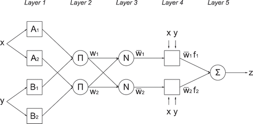
Layer 1: Every node in this layer is an adaptive node with an output defined by:

(1)

(2)

where (or ) is the input to the node and (or ) is a fuzzy set associated with this node. Any continuous and piecewise differentiable function is a qualified candidate for node function in this layer, but usually the chosen membership function is bell-shaped. Parameters in this layer are referred to as premise parameters.

Layer 2: Every node in this layer is a fixed node labelled , which multiplies the incoming signals and sends the product out. For instance:

(3)

Each node output represents the firing strength of a rule. (In fact, according to Jang (1993), other T-norm operators that perform generalized AND can be used as the node function in this layer.)

Layer 3: Every node in this layer is a fixed node labelled . The th node calculates the ratio of the ith rule’s firing strength to the sum of all rules’ firing strengths:

(4)

Outputs of this layer are called normalized firing strengths.

Layer 4: Every node in this layer is an adaptive node with a node function:

(5)

where is the output of Layer 3, and is the parameter set. Parameters in this layer are referred to as consequent parameters.

Layer 5: The single node in this layer is a fixed node labelled , which computes the overall output as the summation of all incoming signals:

(6)

When is a constant, a zero-order Sugeno fuzzy model is obtained, which can be viewed either as a special case of the Mamdani fuzzy inference system (Mamdani and Assilian 1975) or a special case of the Tsukamoto fuzzy model (Tsukamoto 1979). Moreover, a zero-order Sugeno fuzzy model is functionally equivalent to a radial basis function network under certain minor constraints (Jang and Sun 1993). The output of a zero-order Sugeno model is a smooth function of its input variables as long as the neighbouring membership functions in the premise have enough overlap (Jang and Sun 1995).

Wieprecht et al. (2013) used a neuro-fuzzy-based modelling approach for bed load and total bed material load computation of the River Rhine. ANFIS was applied by Azamathulla et al. (2009) for the prediction of bed load in rivers, by Azamathulla et al. (2012) as an alternative approach for the prediction of the functional relationships of sediment transport in sewer pipe systems, and by Azamathulla and Ab. Ghani (2011) for the estimation of the scour depth at culvert outlets. Bakhtyar et al. (2008) employed ANFIS to predict long-shore sediment transport using breaking wave height, breaking angle and wave period as input parameters and generated results superior to those of empirical formulae. In a context different from the present studies, which used macroscopic variables, Valyrakis et al. (2011a) proposed the use of a neuro-fuzzy approach to model the dynamics of entrainment of a coarse particle by rolling due to near-bed turbulent flow structures of different magnitude and duration or frequency and energy content.

Symbolic regression based on genetic programming

Many seemingly different problems in artificial intelligence, symbolic processing and machine learning can be viewed as requiring discovery of a computer program that produces some desired outputs for particular inputs. The process of solving these problems can be reformulated as a search for a highly fit individual computer program in the space of possible ones. Genetic programming extends the concept of genetic algorithms and provides a way to search for this fittest individual computer program (Koza 1992).

GP works by randomly generating a population of computer programs (represented by tree structures) and each individual program in the population is measured in terms of how well it performs in the particular problem environment. This measure is called the fitness measure (Koza 1992) and usually is a sum of errors between the outputs predicted by the program and the actual target values. Initially, the generated computer programs will have exceedingly poor fitness; however, some individuals in the population will turn out to be somewhat fitter than others. These differences in performance are subsequently exploited. The Darwinian principle of reproduction and survival of the fittest, along with the genetic operations of sexual recombination (crossover) and mutation, are used to create a new offspring population of individual programs from the current population. The reproduction principle involves the selection, in proportion to fitness, of a computer program from the current population that survives from the generation by being copied into the new population. The genetic process of sexual recombination is used to create new offspring programs from two parental programs selected in proportion to fitness. The parental programs are typically of different sizes and shapes. The offspring programs are composed of sub-expressions from their parents and are, typically, of different sizes and shapes as well. Intuitively, if two programs are somewhat effective in solving a problem, then some of their parts probably have some merit. By recombining randomly chosen parts of somewhat effective programs, the result may be the production of new programs that are even fitter in solving the problem (Koza 1992). Mutation serves the potentially important role of restoring lost diversity in a population by replacing random subtrees of variable length with other random ones. Its purpose is to prevent premature convergence to unsatisfactory solutions. After the operations of reproduction, crossover and mutation are performed on the current population, the offspring population replaces the old one. Each individual in the new population of programs is then measured for fitness and the process is iterated for a predetermined number of generations. This algorithm will produce populations of programs that over many generations tend to exhibit increasing average fitness in dealing with their environment. The individual computer program that performs best in the evolved generations is considered to be the fittest.

A multigene individual consists of multiple genes, each of which is a GP evolved tree. In multigene symbolic regression, each prediction of the output variable is formed linearly by the weighted output of each of the genes plus a bias term (Searson 2009). Each tree is a function of the input variables. Mathematically, a multigene regression model can be written as:

(7)

where = bias (offset) term; , …, are the gene weights and is the number of genes comprising the current individual. The gene weights are automatically determined by a least squares procedure for each multigene individual. The number and structure of the trees are evolved automatically during a run (subject to user defined constraints) using the training data. Hence, multigene symbolic regression combines the power of classical linear regression with the ability to capture nonlinear behaviour without needing to pre-specify the structure of the nonlinear model and its degree of nonlinearity. During a run, genes are acquired and deleted using a tree crossover operator called two-point high level crossover. This allows the exchange of genes between individuals and it is used in addition to the standard GP recombination operators (Searson et al. 2010).

Genetic programming has been implemented in hydraulic engineering in recent years with very good results. Babovic and Abbott (1997) applied GP to some representative problems, while Babovic and Keijzer (2000) highlighted the usage of GP as a data mining tool in which the human expert interprets models suggested by the computer, aiming at knowledge discovery. Minns (2000) suggests that the symbolic expressions obtained from GP may be less accurate than the ANN in mapping the experimental data; however, these expressions can be more easily examined to provide insights into the processes that created the data. In the context of sediment transport, Zakaria et al. (2010) applied gene-expression programming, which is similar to multigene symbolic regression, to predict the total bed material load for rivers using dimensional quantities from field data, and outperformed some of the traditional sediment load formulae. Ab. Ghani and Azamathulla (2011) employed gene-expression programming as an alternative approach for modelling the functional relationships of sediment transport in sewer pipe systems, whilst Azamathulla et al. (2010) utilized GP to predict the scour depth at bridge piers and obtained results superior to those of ANNs and regression equations. More recently, Ab. Ghani and Azamathulla (2014) developed a functional sediment transport relation for Malaysian rivers by using gene-expression programming with non-dimensional variables, which included a dimensionless mean flow velocity, relative depth and geometric characteristics.

DOMINANT INDEPENDENT VARIABLES FOR OPEN CHANNEL HYDRAULICS AND SEDIMENT TRANSPORT

Sediment load is the material being transported, and it can be divided into wash load and bed material load. The wash load is the fine material of sizes that are not found in appreciable quantities on the bed, and is not considered to be dependent on the local hydraulics of the flow, but instead is dependent on the upstream supply. As a practical definition, the wash load is considered to be the fraction of the sediment load finer than 0.062 mm. The bed material load is the material of sizes that are found in appreciable quantities on the bed; it can be conceptually divided into the bed load (the portion of the load that moves near the bed by means of roll or saltation) and the suspended load (the portion of the load that moves in suspension), although the division is not precise. The consequent difficulty of separating the bed load from the turbulence-dominated suspended load leads to a total load definition for the quantification of sediment transport in sand-bed rivers. A dimensionless, commonly used measure for sediment quantification is concentration by weight in parts per million (ppm), which is the ratio of the sediment discharge to the discharge of the water–sediment mixture, both expressed in terms of mass per unit time, here called . This can be given as:

(8)

where is the water density (kg m^-3), is the sediment density (kg m^-3), is the water discharge (m³ s^-1) and is the volumetric sediment discharge (m³ s^-1). For practical reasons, the density of the water–sediment mixture is taken to be approximately equivalent to the density of water. This approximation will cause errors of less than one percent for concentrations less than 16 000 ppm (Brownlie 1981b).

The parameters governing a sediment transport process can be described by (Yalin 1977):

(9)

where is the mean flow velocity (m s^-1), is the mean flow depth (m), is a characteristic grain diameter (m), is the energy slope (-), is the gravitational acceleration (m s^-2), and is the kinematic viscosity of water (m² s^-1). To ensure dimensional consistency in the derived models, the input and output variables should be dimensionless. Instead of applying dimensional analysis and Buckingham’s π theorem, the independent variables of equation (9) will be introduced by some common and well-known dimensionless variables that have physical meaning and have been utilized for the creation of various sediment transport formulae. These variables are directly related to quantities that the engineer can readily visualize and measure; they are detailed below and summarized in Table 1.

• The Froude number gives a measure of the ratio of inertial forces to gravitational forces of the flow:

  (10)

• The Reynolds number gives a measure of the ratio of inertial forces to viscous forces of the flow:

  (11)

• The shear Reynolds number (Re*), the physical meaning of which is the ratio of particle size to the thickness of the viscous sublayer , because is proportional to :

  (12)

  where is the shear velocity (m s^-1), and is the hydraulic radius (m).

• The dimensionless shear stress or Shields number:

  (13)

  where is the shear stress (kg m^-1 s^-2).

• The dimensionless grain diameter is an expression for grain diameter that can be derived by eliminating shear stress from the two Shields parameters (Shields 1936); or from the drag coefficient and Reynolds number of a settling particle, by eliminating the settling velocity; or dimensionally, with the immersed weight of an individual grain, fluid density, and viscosity as the variables (Ackers and White 1973). The dimensionless grain diameter is, therefore, generally applicable to coarse, transitional, and fine sediments:

  (14)

• The dimensionless stream power equation appears to have first been applied to sediment transport by Rubey (1933) and later by Velikanov (1955). It was again suggested by Knapp (1938), and later introduced by Bagnold (1956) in a paper wherein the flowing fluid was regarded as a transporting machine. The available power supply, or time rate of energy supply, to unit length of a stream is the time rate of liberation in kinetic form of the liquid’s potential energy as it descends the gravity slope . Denoting this power by , Bagnold (1966) derived the formula:

  (15)

  The mean available power supply to the column of fluid over unit bed area, denoted by (kg s^-3), is therefore:

  (16)

  where W is the channel width (m). To define a dimensionless transport parameter that encapsulates Bagnold’s view of sediment transport as a stream power related phenomenon, Eaton and Church (2011) developed the following formula:

  (17)

• Dimensionless unit stream power. Yang (1972) reviewed the basic assumptions used in the derivation of conventional sediment transport equations. He concluded that the assumption that sediment transport rate could be determined from water discharge, average flow velocity, energy slope, or shear stress is questionable. Consequently, the generality and applicability of any equation derived from one of these assumptions is also questionable. The rate of energy per unit weight of water, available for transporting water and sediment in an open channel with reach length x and total drop of , is:

  (18)

  Yang (1972) defines the unit stream power as the velocity-slope product and argues that the rate of work being done by a unit weight of water in transporting sediment must be directly related to the rate of work available to a unit weight of water. Thus, total sediment concentration or total bed material load must be directly related to unit stream power. While Bagnold (1966) emphasized the power that applies to a unit bed area, Yang (1972, 1973) emphasized the power available per unit weight of fluid to transport sediment. The fact that sediment discharge or concentration is dominated by the unit stream power has also been confirmed by Vanoni (1978). While Yang divided unit stream power by fall velocity (m s⁻¹) to obtain a dimensionless variable, Vanoni (1978) divided the product by . Both and are commonly used for describing the size of sediment particles. However, can only reflect the physical size of sediment particles, while can also reflect the interaction between sediment particles and water, which is affected by particle shape, water viscosity and temperature. On the other hand, the computation of fall velocity is problematic and a common source of errors. The emerging variables expressing dimensionless unit stream power according to Yang and Vanoni are, respectively:

  (19)
  (20)

Table 1 Dimensionless variables assessed from the machine learning techniques.

	Dimensionless variables
1	Froude number, Fr
2	Reynolds number, Re
3	Shear Reynolds number, Re*
4	Dimensionless shear stress, τ*
5	Dimensionless grain diameter,
6	Dimensionless stream power, ω*
7	Yang’s dimensionless unit stream power, VS/ωs
8	Vanoni’s dimensionless unit stream power, VS/

DATA PREPARATION

The proper training of a data-driven scheme requires a large number of quality data that represent a wide spectrum of the considered problem. Brownlie’s (1981a) database contains 7027 records (5263 laboratory records and 1764 field records) in 77 data files. These data were subjected to a screening process similar to the one Brownlie (1981b) used for the derivation of his formula, as shown in Table 2, and the measurements that were not verified by Brownlie, were incorrect or incomplete, were removed. In addition, only flume measurements in uniform flows were considered and supercritical flows were removed because subcritical flows usually prevail in nature in sand-bed rivers. Finally, the measurements with specific gravity outside the quartz density range were neglected, and also measurements that had extreme temperature values. Wherever the temperature was missing, values of 15°C and 20°C were used for the calculation of kinematic viscosity in rivers and laboratory flumes, respectively. For the flume data, the sidewall correction of Vanoni and Brooks (1957) was utilized to adjust the hydraulic radius to eliminate the effects of the flume walls.

Table 2 Restrictions imposed on data.

Restriction	Reason
0.062 ≤ d50 ≤ 2.0 mm	Sand only
σg ≤ 5	Eliminate bimodal distributions by restricting the geometric standard deviation of bed particles
W/D > 4	Reduce sidewall effects (only for laboratory data)
R/d50 > 100	Eliminate shallow water effects
Ct > 10 ppm	Accuracy problems associated with low concentration
Fr < 1	Subcritical flows
2.57 ≤ ρs/ρ ≤ 2.68	Natural sediments

Further pruning of the outliers in the training dataset would be beneficial for the training procedure; however, this would be at the expense of the amount of training data, which was already significantly reduced during the screening process. Since most data-driven modelling methods perform well when the data have a distribution that is close to uniform or normal (Pyle 1999), a log-transformation of the input and output variables of all datasets was applied so that the distributions of the transformed variables would be closer to normal. An additional advantage of the log-transformation is that the data-driven models will generate only positive sediment concentrations.

The most popular bed material load equations were developed partially or exclusively from flume data, regression schemes based on dimensionless variables and oversimplification of the physics of the flow. Yang (1973) applied multiple regression analysis for 463 sets of laboratory data for the development of his sediment transport function, Engelund and Hansen’s (1967) equation was developed based on 116 sets of flume data, Ackers and White (1973) developed their formula based on 925 laboratory experiments, the sediment discharge formula of Karim and Kennedy (1990) was obtained from nonlinear regression using a database of 339 river flows and 608 flume flows, and Brownlie (1981b) used 519 field and 480 flume data records in his analysis. Of the total load sediment transport functions, only Molinas and Wu’s (2001) formula was calibrated using only field data of large rivers.

Molinas and Wu (2001) argued that the differences experienced in flow depths, Reynolds numbers, Froude numbers and water surface slopes between large rivers and laboratory flumes affect the resistance to flow as well as sediment wave movement and suspension, and consequently, the transport of sediment. Although the option of developing predictors from field data may seem attractive from a practical perspective, because it presumably avoids scale effects, field data have notable shortcomings in developing physical models. In addition to their relative sparsity, uncertainties in the measurements, not only of the output variables but also of input variables, are generally significantly larger than in the laboratory (Dogan et al. 2009). Moreover, most of the field data may occupy only a small part of the parameter space, while other ranges that may be physically possible but not commonly occurring, such as high flows, may be poorly represented.

The machine learning techniques analysed in the previous section were trained with field as well as with flume data and the generated models were subsequently applied to sediment transport concentration predictions for natural rivers. The data range of the variables that comprise the validation and testing sets are within the data range of those constituting the training set due to the data sensitive nature of the data-driven techniques and the consequent dubiousness of their use to extrapolate.

Training with field data

Data-driven modelling can be considered as an input–output mapping and the subsequent generalization capability is the effect of a good nonlinear interpolation. For this reason, all the datasets (training, validation and testing sets) should have similar statistical distributions to ensure that they come from the same population (Bowden et al. 2002, Bhattacharya et al. 2007). Because the data compilation comprises datasets coming from different researchers, after the screening process, the remaining data were placed in their original order and three consecutive measurements chosen for the training set followed by one for the validation and one for the testing set, in order to obtain a proper representation of all data ranges. This resulted in 521 measurements for training, 174 measurements for validation and 173 measurements for testing. Table 3 shows some statistical measures of these datasets.

Table 3 Statistical measures for the case where the machine learning training was done with field data.

Statistical measures		Fr	Re*	VS/ωs	ω*		(ppm)
Training set
Minimum value	2.113	0.065	2.816	0.0002	0.365	0.094	11
Maximum value	36.95	0.992	113.9	0.093	83.76	3.591	3950
Mean value	9.357	0.280	23.55	0.013	14.68	0.941	671.9
Standard deviation	6.514	0.169	17.08	0.016	15.23	0.591	848
Skewness coefficient	2.072	0.983	2.101	2.258	1.676	0.974	1.765
Validation set
Minimum value	2.126	0.069	2.936	0.0003	0.396	0.102	12.15
Maximum value	36.95	0.846	110.6	0.082	76.62	3.097	3841.3
Mean value	9.371	0.280	23.90	0.012	15.57	0.961	672.9
Standard deviation	6.615	0.167	17.25	0.014	15.75	0.571	817.8
Skewness coefficient	2.111	0.884	2.114	1.868	1.657	0.779	1.602
Testing set
Minimum value	2.575	0.067	3.548	0.0003	0.383	0.097	12.52
Maximum value	36.95	0.915	112.7	0.090	78.34	3.180	3662.8
Mean value	9.775	0.282	24.51	0.013	13.68	0.902	702.7
Standard deviation	6.682	0.169	17.49	0.016	14.72	0.578	915.9
Skewness coefficient	1.988	0.875	2.066	2.213	1.992	1.070	1.661

Training with flume data

In this case, since measurements in natural streams and rivers are notoriously difficult, and sometimes inaccurate, and the inclusion of field data in the training set would result in a model applicable only to rivers similar to those the data were obtained from, field data were excluded from the training set. Consequently, the training set consists solely of laboratory flume data so that the noise embedded in the training set is minimized. In the context of machine learning, Dogan et al. (2009) constructed relevance vector machine based probabilistic models and Kitsikoudis et al. (2013) employed ANNs and SR to address the issue of transferability of a model that is trained solely on flume data and subsequently implemented on river data, with very good results. This approach assumes similarity of the flow in different scales. The main difference between a laboratory flume and a natural river is probably the increased slope of the flume and the subsequent difference in roughness, bed forms and resistance to the flow. However, the majority of the observed bed forms in the flume data are either ripples or dunes, so the mechanism for resistance to flow due to bed forms should be similar to that of natural rivers, since dunes are the predominant bed forms that occur in nature (Vanoni 2006). As a result, there were 973 flume measurements for training, 262 field measurements for validation and 262 field measurements for testing. Table 4 shows some statistical measures of these datasets.

Table 4 Statistical measures for the case where the machine learning training was done with flume data.

Statistical measures	dgr	Fr	Re*	VS/ωs	ω*	τ*	Ct (ppm)
Flume data
Training set
Minimum value	2.405	0.166	2.468	0.001	0.093	0.032	10.20
Maximum value	38.80	0.999	107.9	0.211	49.13	1.874	10630
Mean value	10.05	0.484	17.91	0.027	4.615	0.433	815.0
Standard deviation	6.514	0.180	16.35	0.031	6.540	0.323	1283.1
Skewness coefficient	1.591	0.951	2.874	2.440	3.027	1.070	3.154
Field data
Validation set
Minimum value	3.924	0.166	6.466	0.002	0.365	0.094	11
Maximum value	36.95	0.942	100.3	0.075	49.04	1.854	7240
Mean value	11.22	0.364	27.82	0.016	9.879	0.791	1016.1
Standard deviation	7.29	0.144	17.50	0.013	9.201	0.437	1152.4
Skewness coefficient	1.717	1.105	1.832	1.709	1.472	0.273	2.171
Testing set
Minimum value	3.171	0.167	6.165	0.002	0.376	0.097	24
Maximum value	36.95	0.992	103.9	0.087	48.28	1.844	7230
Mean value	10.98	0.368	27.09	0.017	10.36	0.809	1048.2
Standard deviation	7.297	0.147	17.10	0.013	9.765	0.437	1186.2
Skewness coefficient	1.805	1.202	1.927	1.790	1.644	0.219	2.112

APPLICATIONS

The determination of the input parameters for the machine learning schemes is made on the basis of a tentative assessment through a trial-and-error procedure. From the techniques proposed, the trial-and-error process is accomplished with the aid of ANNs, due to their speed, and after the determination of the most promising combinations that may serve as inputs, the other machine learning techniques are implemented too. The most potent input variable combinations, which will be applied to the data-driven schemes, seem to be those listed in Table 5. These combinations include the independent variables of equation (9) and others that are relatively easily measured and commonly used in engineering.

Table 5 Input combinations implemented in this study.

	Input combinations
(a)	, , , VS/ωs
(b)	, ,
(c)	, ,

It is noteworthy that all three combinations (Table 5) include dimensionless grain diameter and Froude number, among others. Whilst the Froude number gives a measure of the ratio of inertial forces to gravitational forces of the flow and is a commonly used variable in hydraulic engineering, the potential usage of dimensionless grain diameter is twofold. First, it introduces kinematic viscosity and median grain diameter, and secondly provides a variable with distribution close to normal for the input data. The necessity for the provided normal distribution can be seen from Combination (a) where the shear Reynolds number, which essentially includes dimensionless grain diameter, is also included. The absence of any of these two terms in Combination (a) has detrimental effects in the predictive capability of the generated model. The other variables in the combinations examined here are those that most sediment transport formulae rely heavily on, namely the dimensionless unit stream power, the dimensionless stream power and the dimensionless shear stress. For combination (a), Yang’s dimensionless unit stream power performed better than Vanoni’s and consequently was preferred, despite the fact that the calculation of fall velocity may be problematic. The other two combinations, (b) and (c), comprise just three variables because shear is embedded in dimensionless stream power and dimensionless shear stress, respectively.

A criterion for the initiation of motion has been omitted due to the stochastic nature of the phenomenon caused by turbulence fluctuations. Paintal (1971), in a series of experiments, indicated that a distinct condition for the beginning of movement does not exist. At very low shear stresses, the possibility of movement becomes very small but never equals zero. Lavelle and Mofjeld (1987) argued that under turbulent fluid motion at a sediment bed, some particle movement must occur at all non-zero time mean velocities. Valyrakis et al. (2011b, 2013) explored the fluctuating nature of the applied hydrodynamic forces and introduced impulse and energy concepts that are compatible to the dynamic character of particle transport, by accounting for the temporal dimension of high-magnitude turbulent events and could potentially be applied as a threshold criterion on an event-based machine learning framework. However, the most common criterion for the initiation of motion based on averaged criteria, especially in field applications, is that proposed by Shields (1936), modifications of which were proposed by several researchers based on . As a result, since the critical shear stress value is obtained from , an estimation of the effective portion of the flow that quantifies the sediment transport rate is feasible. In sand-bed rivers, the shear stress that is exerted on the bed can be well above the threshold, in bankfull conditions, and in this case neglecting a threshold will introduce a negligible error. This is corroborated by Yang (1979) who introduced a unit stream power equation for relatively high sediment concentrations without a criterion for the incipience of motion, which after a detailed statistical comparison with his classic formula (Yang 1973) proved equally accurate for concentrations that exceed 100 ppm.

The optimal configuration of each machine learning scheme is considered to be the one that performs best in the validation set. With this approach, the testing set remains unseen during the training procedure and the generalization capability of the schemes is subsequently evaluated. The evaluation of the modelled results with respect to the observed ones is made on the basis of the root mean square error (RMSE):

(21)

mean absolute error (MAE):

(22)

mean normalized error (MNE):

(23)

and the Nash and Sutcliffe (1970) coefficient of efficiency (CE):

(24)

where is the mean observed value. DR is the discrepancy ratio; i.e. the percentage of the calculated concentrations that lie within one half (or a quarter) and two (or four) times the respective measured concentrations. In addition to the above, parsimonious models with simpler structure were preferred over complicated ones with similar or even slightly better performance.

ANN application

For the ANN application, the computational tool is provided by the MATLAB neural network toolbox (Demuth et al. 2009). Due to the importance of the initial values of the synaptic weights in the search for local minima of the error function, a supplementary MATLAB code was written that determines the most efficient ANN, which is the one that performs best in the validation set, within 2000 training executions, for each network architecture tested, with random initial weights for every repetition. The training function is the Levenberg-Marquardt back-propagation algorithm (Hagan and Menhaj 1994) and the error function is the mean square error between calculated and observed values. The neurons of the hidden layer(s) will have the hyperbolic tangent activation function, which squashes the data into the range (−1, 1), and the single neuron of the output layer will have the linear activation function (Hornik et al. 1989). The applied data are scaled to the range (−0.9, 0.9) because, if the values are scaled to the extreme limits of the transfer function, the size of the weight updates is extremely small and flat-spots in training are likely to occur (Maier and Dandy 2000).

Maier and Dandy (1998) provided a valuable guide on the behaviour of back-propagation ANNs under a wide range of operating conditions, although for a particular case study (forecasting salinity in the River Murray). The results obtained, indicate that learning rate, momentum, the gain of the transfer function, epoch size and network geometry have a significant impact on training speed, but not on generalization ability. For this reason, the values of these variables used in this paper are those provided by default by the MATLAB neural network toolbox (Demuth et al. 2009).

ANFIS application

The computational tool for the ANFIS application is provided by the MATLAB fuzzy logic toolbox. It supports only Sugeno-type systems, and these must have the following properties:

• Be first or zero-th order Sugeno-type systems.

• Have a single output, obtained using weighted average defuzzification. All output membership functions must be of the same type and either be linear or constant.

• Have no rule sharing. Different rules cannot share the same output membership function; i.e. the number of output membership functions must be equal to the number of rules.

• Have unity weight for each rule.

The fuzzy logic toolbox uses a hybrid learning algorithm to identify parameters of Sugeno-type fuzzy inference systems. It applies a combination of the least-squares method and the back-propagation gradient descent method for training FIS membership function parameters to emulate a given training dataset (Jang 1993, Jang and Sun 1995), whilst the error function is the sum of squared errors. The ANFIS architecture and the membership functions associated with each respective input are determined after a trial-and-error process, whilst the training options used are the program defaults.

SR application

GPTIPS (Searson 2009) is an open source MATLAB toolbox that performs multigene symbolic regression based on genetic programming. For its proper implementation, some custom modifications must be made to interchangeable parameters in order to deal with the peculiarities of the problem under consideration. Table 6 shows the parameters and genetic operator configurations that were tested. Searson et al. (2010) have found that enforcing stringent tree depth restrictions often allows the evolution of relatively compact models that are linear combinations of low order nonlinear transformations.

Table 6 Parameters and genetic operators configurations tested in GPTIPS.

Parameters and genetic operators	Adjustments
Population size	7500
Number of generations	200
Max genes	2–3
Max gene tree depth	4–6
Functions
Probability of GP mutation event	0.35
Probability of GP crossover event	0.60
Probability of GP direct copy event	0.05
Error function	Root mean square error

Table 7 Performance evaluation indices of the techniques utilized for the case where the machine learning training was done with field data.

	RMSE (ppm)	MAE (ppm)	MNE (%)	CE	(%)	(%)
Training set
ANN(a)	391.11	212.54	44.05	0.787	85.99	98.46
ANN(b)	413.32	219.36	48.07	0.762	81.77	96.74
ANN(c)	418.75	228.82	50.66	0.756	81.57	96.74
ANFIS(a)	426.94	229.84	49.15	0.746	82.15	97.70
ANFIS(b)	401.31	222.57	48.79	0.776	82.34	97.50
ANFIS(c)	413.08	222.60	51.37	0.762	81.19	97.50
SR(a)	449.56	242.12	52.93	0.718	79.27	96.55
SR(b)	460.93	246.94	53.90	0.704	78.89	96.55
SR(c)	435.51	235.52	56.25	0.736	78.12	96.16
Validation set
ANN(a)	430.07	230.99	42.68	0.722	81.61	98.28
ANN(b)	419.22	222.30	46.03	0.736	81.61	97.70
ANN(c)	430.02	229.06	44.19	0.722	81.61	98.28
ANFIS(a)	457.61	236.59	43.97	0.685	81.61	96.55
ANFIS(b)	455.76	238.01	43.81	0.688	80.46	95.98
ANFIS(c)	478.84	247.33	47.47	0.655	78.16	94.83
SR(a)	477.26	251.95	48.20	0.657	77.01	94.25
SR(b)	477.49	247.09	48.10	0.657	79.31	94.83
SR(c)	493.99	258.03	50.33	0.633	78.16	94.25
Testing set
ANN(a)	452.04	207.87	45.62	0.755	79.77	95.95
ANN(b)	478.06	234.57	45.52	0.726	80.35	96.53
ANN(c)	452.94	219.73	45.37	0.754	80.92	98.27
ANFIS(a)	492.74	235.89	43.51	0.709	80.92	97.11
ANFIS(b)	498.98	244.87	45.95	0.701	80.92	97.69
ANFIS(c)	495.15	240.15	45.81	0.706	78.61	97.11
SR(a)	515.04	250.63	49.24	0.682	78.03	97.69
SR(b)	515.63	248.62	47.04	0.681	80.92	97.69
SR(c)	506.36	248.32	48.58	0.693	77.46	96.53

RESULTS AND DISCUSSION

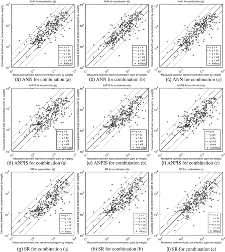
The machine learning techniques generated the results for the training, validation and testing sets shown in Tables 7 and 8, for the cases where the training set comprised solely field and flume data, respectively. The results of the proposed models, for the testing set, are depicted in the scatter plots of Figs 2 and 3, whilst Tables 9 and 10 show a comparison, in the testing set, of the aforementioned models with the Ackers and White (1973), Brownlie (1981b), Engelund and Hansen (1967), Karim and Kennedy (1990), Molinas and Wu (2001), and Yang (1973) formulae, for the cases of training with field and flume data, respectively. The formulae of Brownlie (1981b) and Karim and Kennedy (1990) have the significant advantage that they were calibrated with some of the data utilized for this comparison. The optimal architecture of the ANNs comprises one hidden layer for all the cases and the number of hidden neurons is displayed in Table 11, whilst Table 12 shows the optimal configurations for the models derived from ANFIS, for all the aforementioned combinations. The equations generated from SR are displayed in the Appendix, equations (A1)–(A6).

Table 8 Performance evaluation indices of the techniques utilized for the case where the machine learning training was done with flume data.

	RMSE (ppm)	MAE (ppm)	MNE (%)	CE	(%)	(%)
Flume data
Training set
ANN(a)	768.43	334.60	76.11	0.641	74.82	95.27
ANN(b)	788.12	317.51	64.23	0.622	77.08	96.09
ANN(c)	787.67	315.34	69.07	0.623	76.67	95.07
ANFIS(a)	675.90	251.84	46.05	0.722	81.81	97.94
ANFIS(b)	734.63	297.07	50.47	0.672	79.45	97.33
ANFIS(c)	673.24	270.73	45.60	0.724	82.73	98.25
SR(a)	725.52	282.08	50.00	0.680	80.58	97.33
SR(b)	732.03	295.08	54.26	0.674	78.01	96.61
SR(c)	712.72	278.42	49.67	0.691	81.40	97.23
Field data
Validation set
ANN(a)	828.43	459.37	68.94	0.481	70.61	92.37
ANN(b)	820.01	442.96	63.71	0.492	72.52	94.66
ANN(c)	826.80	443.24	56.64	0.483	70.23	92.75
ANFIS(a)	933.85	538.44	79.62	0.341	62.98	88.17
ANFIS(b)	903.48	487.97	62.08	0.383	66.79	90.08
ANFIS(c)	937.57	517.12	65.84	0.336	64.12	89.69
SR(a)	962.84	536.12	55.82	0.299	61.45	87.02
SR(b)	890.58	481.85	63.15	0.400	68.70	91.22
SR(c)	925.10	508.82	61.41	0.353	67.18	90.08
Testing set
ANN(a)	845.17	466.12	58.46	0.490	72.52	94.27
ANN(b)	850.83	464.46	54.80	0.484	75.57	95.04
ANN(c)	864.85	466.44	50.17	0.466	70.61	95.04
ANFIS(a)	977.90	548.63	66.56	0.318	65.65	89.31
ANFIS(b)	961.00	507.55	53.77	0.341	67.94	92.75
ANFIS(c)	994.17	530.92	57.46	0.295	66.79	90.46
SR(a)	992.42	535.29	49.61	0.297	65.65	92.37
SR(b)	973.24	524.41	59.34	0.324	70.61	93.13
SR(c)	980.59	517.64	55.35	0.314	70.61	93.13

Table 9 Comparison of the machine learning schemes, which were trained with field data, with some sediment transport formulae for the test set.

	(ppm)	(ppm)	(%)	CE	(%)	(%)
Ackers and White (1973)	720.56	359.40	51.02	0.381	57.56	90.12
Brownlie (1981b)	648.44	322.17	45.78	0.496	68.79	94.22
Engelund and Hansen (1967)	637.96	336.12	57.43	0.522	67.07	91.62
Karim and Kennedy (1990)	767.41	383.88	64.13	0.294	62.43	90.75
Molinas and Wu (2001)	726.47	387.76	68.80	0.367	58.38	91.33
Yang (1973)	724.24	396.81	61.19	0.371	42.20	72.25
ANN(a)	452.04	207.87	45.62	0.755	79.77	95.95
ANN(b)	478.06	234.57	45.52	0.726	80.35	96.53
ANN(c)	452.94	219.73	45.37	0.754	80.92	98.27
ANFIS(a)	492.74	235.89	43.51	0.709	80.46	97.11
ANFIS(b)	498.98	244.87	45.95	0.701	80.46	97.69
ANFIS(c)	495.15	240.15	45.81	0.706	78.61	97.11
SR(a)	515.04	250.63	49.24	0.682	78.03	97.69
SR(b)	515.63	248.62	47.04	0.681	80.92	97.69
SR(c)	506.36	248.32	48.58	0.693	77.46	96.53

Table 10 Comparison of the machine learning schemes, which were trained with flume data, with some sediment transport formulae for the test set.

	(ppm)	(ppm)	(%)	CE	(%)	(%)
Ackers and White (1973)	1016.7	552.47	48.60	0.268	59.30	92.64
Brownlie (1981b)	1037.7	531.49	49.41	0.232	68.70	91.98
Engelund and Hansen (1967)	1007.1	536.41	63.29	0.283	71.43	92.28
Karim and Kennedy (1990)	972.98	507.82	67.44	0.325	70.23	91.98
Molinas and Wu (2001)	1145.4	658.58	84.78	0.064	54.58	87.40
Yang (1973)	1177.7	664.76	64.33	0.010	49.62	84.35
ANN(a)	845.17	466.12	58.46	0.490	72.52	94.27
ANN(b)	850.83	464.46	54.80	0.484	75.57	95.04
ANN(c)	864.85	466.44	50.17	0.466	70.61	95.04
ANFIS(a)	977.90	548.63	66.56	0.318	65.65	89.31
ANFIS(b)	961.00	507.55	53.77	0.341	67.94	92.75
ANFIS(c)	994.17	530.92	57.46	0.295	66.79	90.46
SR(a)	992.42	535.29	49.61	0.297	65.65	92.37
SR(b)	973.24	524.41	59.34	0.324	70.61	93.13
SR(c)	980.59	517.64	55.35	0.314	70.61	93.13

Table 11 Number of neurons in the single hidden layer of the optimal ANNs architectures.

Combination	Number of hidden neurons
	Training with field data	Training with flume data
(a)	11	4
(b)	9	5
(c)	7	6

Table 12 Optimal ANFIS configurations.

Combination	Number of MFs	Type of MFs	Number of rules	Type of output function
Training with field data
(a)	2	Gaussian curve	16	constant
(b)	2	Bell-shaped	8	constant
(c)	2	Gaussian curve	8	linear
Training with flume data
(a)	2	Gaussian curve	16	constant
(b)	2	Gaussian curve	8	constant
(c)	2	Gaussian curve	8	constant

Fig. 2 Scatter plots of measured and calculated sediment concentrations for the test set of the case where the regression schemes were trained with field data. (a)–(c) ANN for combinations (a)–(c), respectively; (d)–(f) ANFIS for combinations (a)–(c), respectively; (g)–(i) SR for combinations (a)–(c), respectively.

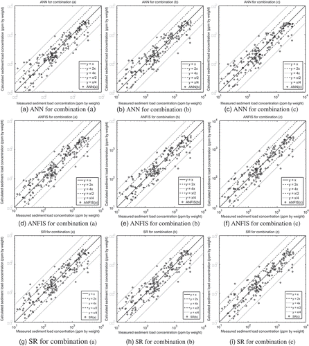
Fig. 3 Scatter plots of measured and calculated sediment concentrations for the test set of the case where the regression schemes were trained with flume data. (a)–(c) ANN for combinations (a)–(c), respectively; (d)–(f) ANFIS for combinations (a)–(c), respectively; (g)–(i) SR for combinations (a)–(c), respectively.

Models with augmented complexity were tested and it was observed that while the training time kept increasing, the model generalization performance did not improve significantly and sometimes deteriorated because of overfitting to the training data. Specifically, the tested ANN architectures comprised one or two hidden layers with a maximum of 20 neurons in each one, while the tested ANFIS models used two or three membership functions for each input and the maximum training epochs were set to 20 000. This increased complexity effect was especially pronounced in the SR implementation, where it was observed that a large population size or number of generations rendered the training process very slow, while bigger genes led to highly nonlinear models that fail to generalize sufficiently. In fact, this can be confirmed with the applied cross-validation concept where the model selection is based on the performance in the validation set and showed that simpler models generalize equally well or even better than the complicated ones, and there is no need for additional elaboration or extended training time, which may cause overfitting to the training data. On the basis of this observation, model structures of higher complexity were not investigated further.

All the machine learning schemes that were trained with field data generate results superior to those of the aforementioned formulae for almost all the performance measures used, as can be seen in Table 9. From the schemes that were trained with flume data, the results obtained from ANNs surpass those of the common formulae, while those obtained from ANFIS and SR are of the same order (Table 10). Highly nonlinear models derived from SR were excluded from the comparison, despite their good performance. While the Ackers and White (1973) formula is valid for and the Engelund and Hansen (1967) formula is valid for mm, they are included in the same tables as the other formulae due to space limitations; however, they displayed about the same discrepancy as the machine learning schemes either way. Extensive comparisons of the sediment transport formulae can be found in Alonso et al. (1981), Brownlie (1981b), Nakato (1990), and Yang (2003).

It seems that every combination used has its own merit, since they produce similarly good results, with respect to the data-driven technique employed. Despite the fundamental differences of the independent variables used, such as the fact that shear stress is a vector while both stream power and unit stream power are scalar quantities or the fact that while stream power emphasizes the power that applies to a unit bed area, unit stream power emphasizes the power available per unit weight of fluid to transport sediment, each of these concepts has similar potential for the quantification of the phenomenon, according to Tables 7 and 8 where they produce similarly good results, probably because their derivation is based on some common variables. Finally, especially for the case where the training is made with flume data and the derived models are applied to actual rivers, with significant differences in their statistical distributions, machine learning exhibits its ability to capture functions with physical meaning.

Although these results cannot be considered conclusive, it seems that ANNs yield better results compared to those of ANFIS and SR. This happens partially due to the fact that ANN training is much faster than the time consuming GP training, and in a given time they can do multiple runs compared to GP, resulting in the exploration of many local minima of the error function. Whilst ANNs have this property, GP training is based on a stochastic concept seeking the global optimum. Searson (2009) argues that GPTIPS sometimes, usually when only a few input variables are involved, lags behind a neural network model in terms of raw predictive performance, but the equivalent GP models are often simpler, shorter and may be more transparent and open to physical interpretation. This conclusion is valid for this study as well, and especially when the training is done with flume data, the formulae derived from SR are really simple, probably because of the uniform flows and the controlled environment under which the data were retrieved, as shown in the Appendix in equations (A4)–(A6) compared to equations (A1)–(A3), which were derived from field data. These formulations are considered to be empirical and their physical interpretation is based on the variables presented in equations (10)–(20) and their weight in the rendered formulae.

Analysis of laboratory experiments for the determination of sediment transport rate performed under similar flow conditions, made by van Rijn (1982), showed deviations by up to a factor of two, and based on these results he concluded that it seems hardly possible to predict the total load with an inaccuracy of less than a factor two. Eidsvik (2004) argued that even in the simplest equilibrium flow over a flat bottom, the minimum sediment transport prediction error is estimated to be comparable to a factor of two, whilst for more complicated flows the prediction error is even higher. Based on these arguments, the results obtained from machine learning are satisfactory, since, as can be seen in Tables 7 and 8, DR values are high, RMSE and MNE values are low, while MAE values are small compared to the mean values shown in Tables 3 and 4.

CONCLUSIONS

This paper shows the quality of machine learning and the potential of three fundamental concepts, widely applied in the field of sediment transport, namely shear stress, stream power, and unit stream power, based on techniques such as artificial neural networks, symbolic regression based on genetic programming, and adaptive-network-based fuzzy inference system. Each of these sediment transport quantification approaches has its own merit, since all three produce similarly good results, when they are utilized as averaged macroscopic variables, with respect to the data-driven modelling technique employed.

The regression schemes were trained with field data, following the work of previous researchers, as well as with flume data, to address the issue of transferability of a model trained from flume data to an actual river and examine the efficiency of the machine learning techniques in capturing the semantics of this natural phenomenon without overfitting to the training data. The results obtained from schemes trained with field data are superior to those of the commonly used sediment transport formulae for all the performance indices used for evaluation, whilst those derived from schemes trained with flume data are better or at least comparable to the results derived from the common sediment transport formulae, depending on the machine learning technique used. However the generalisation capability of the flume trained models was tested on a more stringent basis since the field trained models were trained, validated, and tested in the same rivers with data that have similar statistical distributions.

The models that were derived from field data produce better results than those obtained from the models trained with flume data, as was expected. However, the functions generated from the flume data are much simpler and parsimonious, especially for the symbolic regression modelling. This is probably due to the uniform flow data retrieved from flumes, which constitute the training set. Of the machine learning techniques considered, artificial neural networks gave the best results, but the formulae obtained from symbolic regression are simpler and more transparent.

Disclosure statement

No potential conflict of interest was reported by the author(s).

Acknowledgements

The authors would like to thank H. Md. Azamathulla and an anonymous reviewer whose suggestions and constructive comments improved the presentation of this paper.

APPENDIX

The following equations (A1)–(A3) are the results of symbolic regression, trained with field data for the input combinations (a)–(c), of Table 5, respectively.

(A1)

(A2)

(A3)

The following equations (A4)–(A6) are the results of symbolic regression, trained with flume data for the input combinations (a)–(c), of Table 5, respectively.

(A4)

(A5)

(A6)

REFERENCES

- Ab. Ghani, A. and Azamathulla, H.M., 2011. Gene-expression programming for sediment transport in sewer pipe systems. Journal of Pipeline Systems Engineering and Practice, 2 (3), 102–106. doi:10.1061/(ASCE)PS.1949-1204.0000076
- Ab. Ghani, A. and Azamathulla, H.M., 2014. Development of GEP-based functional relationship for sediment transport in tropical rivers. Neural Computing and Applications, 24 (2), 271–276. doi:10.1007/s00521-012-1222-9
- Ackers, P. and White, W.R., 1973. Sediment transport: new approach and analysis. Journal of the Hydraulics Division, 99 (HY11), 2041–2060.
- Alonso, C.V., Neibling, W.H., and Foster, G.R., 1981. Estimating sediment transport capacity in watershed modeling. Transactions, ASAE, 24 (5), 1211–1220. doi:10.13031/2013.34422
- Azamathulla, H.M. and Ab. Ghani, A., 2011. ANFIS-based approach for predicting the scour depth at culvert outlets. Journal of Pipeline Systems Engineering and Practice, 2 (1), 35–40. doi:10.1061/(ASCE)PS.1949-1204.0000066
- Azamathulla, H.M., Ab. Ghani, A., and Fei, S.Y., 2012. ANFIS-based approach for predicting sediment transport in clean sewer. Applied Soft Computing, 12 (3), 1227–1230. doi:10.1016/j.asoc.2011.12.003
- Azamathulla, H.M., et al., 2010. Genetic programming to predict bridge pier scour. Journal of Hydraulic Engineering, 136 (3), 165–169. doi:10.1061/(ASCE)HY.1943-7900.0000133
- Azamathulla, H.M., et al., 2009. An ANFIS-based approach for predicting the bed load for moderately sized rivers. Journal of Hydro-Environment Research, 3 (1), 35–44. doi:10.1016/j.jher.2008.10.003
- Babovic, V., 2000. Data mining and knowledge discovery in sediment transport. Computer Aided Civil and Infrastructure Engineering, 15 (5), 383–389. doi:10.1111/0885-9507.00202
- Babovic, V. and Abbott, M.B., 1997. The evolution of equations from hydraulic data. Part II: applications. Journal of Hydraulic Research, 35 (3), 411–430. doi:10.1080/00221689709498421
- Babovic, V. and Keijzer, M., 2000. Genetic programming as a model induction engine. Journal of Hydroinformatics, 2 (1), 35–60.
- Bagnold, R.A., 1956. The flow of cohesionless grains in fluids. Philosophical Transactions of the Royal Society of London, Series A, 249 (964), 235–297. doi:10.1098/rsta.1956.0020
- Bagnold, R.A., 1966. An approach to the sediment transport problem from general physics. Prof. Paper 422-I, U.S. Geological Survey.
- Bakhtyar, R., et al., 2008. Long-shore sediment transport estimation using fuzzy inference system. Applied Ocean Research, 30 (4), 273–286. doi:10.1016/j.apor.2008.12.001
- Bhattacharya, B., Price, R.K., and Solomatine, D.P., 2005. Data driven modeling in the context of sediment transport. Physics and Chemistry of the Earth, 30 (4–5), 297–302. doi:10.1016/j.pce.2004.12.001
- Bhattacharya, B., Price, R.K., and Solomatine, D.P., 2007. Machine learning approach to modeling sediment transport. Journal of Hydraulic Engineering, 133 (4), 440–450. doi:10.1061/(ASCE)0733-9429(2007)133:4(440)
- Bowden, G.J., Maier, H.R., and Dandy, G.C., 2002. Optimal division of data for neural networks models in water resources applications. Water Resources Research, 38 (2), 2–11. doi:10.1029/2001WR000266
- Brownlie, W.R., 1981a. Compilation of alluvial channel data: laboratory and field. Pasadena, CA: Tech. Rep. KH-R-43B, W.M. Keck Laboratory of Hydraulics and Water Resources, California Institute of Technology.
- Brownlie, W.R., 1981b. Prediction of flow depth and sediment discharge in open channels. Pasadena, CA: Tech. Rep. KH-R-43A, W.M. Keck Laboratory of Hydraulics and Water Resources, California Institute of Technology.
- Demuth, H.B., Beale, M.H., and Hagan, M.T., 2009. Neural network toolbox: for use with MATLAB. Natick, MA: The Mathworks Inc.
- Dogan, E., et al., 2009. From flumes to rivers: can sediment transport in natural alluvial channels be predicted from observations at the laboratory scale? Water Resources Research, 45 (8), W08433. doi:10.1029/2008WR007637
- Eaton, B.C. and Church, M., 2011. A rational sediment transport scaling relation based on dimensionless stream power. Earth Surface Processes and Landforms, 36 (7), 901–910. doi:10.1002/esp.2120
- Eidsvik, K.J., 2004. Some contributions to the uncertainty of sediment transport predictions. Continental Shelf Research, 24 (6), 739–754. doi:10.1016/j.csr.2003.11.003
- Einstein, H.A., 1942. Formulas for the transportation of bed load. Transactions, ASCE, 107 (2140), 561–573.
- Engelund, F. and Hansen, E., 1967. A monograph on sediment transport in alluvial streams. Copenhagen: Teknisk Forlag.
- Hagan, M.T. and Menhaj, M.B., 1994. Training feedforward networks with the Marquardt algorithm. IEEE Transactions on Neural Networks, 5 (6), 989–993. doi:10.1109/72.329697
- Haykin, S., 2009. Neural networks and learning machines. 3rd ed. Upper Saddle River, NJ: Prentice Hall.
- Hornik, K., Stinchcombe, M., and White, H., 1989. Multilayer feedforward networks are universal approximators. Neural Networks, 2 (5), 359–366. doi:10.1016/0893-6080(89)90020-8
- Jang, J.-S.R., 1993. ANFIS: adaptive-network-based fuzzy inference system. IEEE Transactions on Systems, Man, and Cybernetics, 23 (3), 665–685. doi:10.1109/21.256541
- Jang, J.-S.R. and Sun, C.-T., 1993. Functional equivalence between radial basis function networks and fuzzy inference systems. IEEE Transactions on Neural Networks, 4 (1), 156–159. doi:10.1109/72.182710
- Jang, J.-S.R. and Sun, C.-T., 1995. Neuro-fuzzy modeling and control. Proceedings of the IEEE, 83 (3), 378–406. doi:10.1109/5.364486
- Karim, M.F. and Kennedy, J.F., 1990. Menu of coupled velocity and sediment- discharge relations for rivers. Journal of Hydraulic Engineering, 116, 978–996. doi:10.1061/(ASCE)0733-9429(1990)116:8(978)
- Kitsikoudis, V., Sidiropoulos, E., and Hrissanthou, V., 2013. Derivation of sediment transport models for sand bed rivers from data-driven techniques. In: A. Manning, ed. Sediment transport processes and their modelling applications. Rijeka: InTech Publishing Company, 277–308.
- Knapp, R.T., 1938. Energy balance in stream flows carrying suspended load. Transactions, American Geophysical Union, 19 (1), 501–505. doi:10.1029/TR019i001p00501
- Koza, J.R., 1992. Genetic programming: on the programming of computers by means of natural selection. Cambridge, MA: MIT Press.
- Lavelle, J.W. and Mofjeld, H.O., 1987. Do critical stresses for incipient motion and erosion really exist? Journal of Hydraulic Engineering, 113 (3), 370–385. doi:10.1061/(ASCE)0733-9429(1987)113:3(370)
- Lin, B. and Namin, M.M., 2005. Modelling suspended sediment transport using an integrated numerical and ANNs model. Journal of Hydraulic Research, 43 (3), 302–310. doi:10.1080/00221680509500124
- Maier, H.R. and Dandy, G.C., 1998. The effect of internal parameters and geometry on the performance of back-propagation neural networks: an empirical study. Environmental Modelling and Software, 13 (2), 193–209. doi:10.1016/S1364-8152(98)00020-6
- Maier, H.R. and Dandy, G.C., 2000. Neural networks for the prediction and fore- casting of water resources variables: a review of modeling issues and applications. Environmental Modelling and Software, 15 (1), 101–124.
- Mamdani, E.H. and Assilian, S., 1975. An experiment in linguistic synthesis with a fuzzy logic controller. International Journal of Man-Machine Studies, 7 (1), 1–13. doi:10.1016/S0020-7373(75)80002-2
- Minns, A.W., 2000. Subsymbolic methods for data mining in hydraulic engineering. Journal of Hydroinformatics, 2 (1), 3–13.
- Molinas, A. and Wu, B., 2001. Transport of sediment in large sand-bed rivers. Journal of Hydraulic Research, 39 (2), 135–146. doi:10.1080/00221680109499814
- Nagy, H.M., Watanabe, K., and Hirano, M., 2002. Prediction of sediment load concentration in rivers using artificial neural network model. Journal of Hydraulic Engineering, 128 (6), 588–595. doi:10.1061/(ASCE)0733-9429(2002)128:6(588)
- Nakato, T., 1990. Tests of selected sediment-transport formulas. Journal of Hydraulic Engineering, 116 (3), 362–379. doi:10.1061/(ASCE)0733-9429(1990)116:3(362)
- Nash, J.E. and Sutcliffe, J.V., 1970. River flow forecasting through conceptual models, Part I—a discussion of principles. Journal of Hydrology, 10 (3), 282–290. doi:10.1016/0022-1694(70)90255-6
- Paintal, A.S., 1971. Concept of critical shear stress in loose boundary open channels. Journal of Hydraulic Research, 9 (1), 91–113. doi:10.1080/00221687109500339
- Pyle, D., 1999. Data preparation for data mining. San Francisco, CA: Morgan Kaufmann.
- Rubey, W.W., 1933. Equilibrium conditions in debris-laden streams. Transactions, American Geophysical Union, 14 (1), 497–505. doi:10.1029/TR014i001p00497
- Rumelhart, D.E., Hinton, G.E., and Williams, R.J., 1986. Learning representations of back-propagation errors. Nature, 323 (6088), 533–536. doi:10.1038/323533a0
- Searson, D.P., 2009. GPTIPS: Genetic Programming and Symbolic Regression for MATLAB, User Guide.
- Searson, D.P., Leahy, D.E., and Willis, M.J., 2010. GPTIPS: an open source genetic programming toolbox for multigene symbolic regression. In: S.I. Ao, et al., eds. Proceedings of the international multiconference of engineers and computer scientists. Vol. I. Hong Kong: Newswood Limited.
- Shields, A.F., 1936. Application of similarity principles and turbulence research to bedload movement. Transl. into English by Ott, W.P. and van Uchelen, J.C., California Institute of Technology, Pasadena, CA.
- Solomatine, D.P. and Ostfeld, A., 2008. Data-driven modelling: some past experiences and new approaches. Journal of Hydroinformatics, 10 (1), 3–22. doi:10.2166/hydro.2008.015
- Sugeno, M. and Kang, G.T., 1988. Structure identification of fuzzy model. Fuzzy Sets and Systems, 28 (1), 15–33. doi:10.1016/0165-0114(88)90113-3
- Syvitski, J.P.M., et al., 2005. Impact of humans on the flux of terrestrial sediment to the global coastal ocean. Science, 308 (5720), 376–380. doi:10.1126/science.1109454
- Takagi, T. and Sugeno, M., 1985. Fuzzy identification of systems and its applications to modeling and control. IEEE Transactions on Systems, Man, and Cybernetics, 15 (1), 116–132.
- Tsukamoto, Y., 1979. An approach to fuzzy reasoning method. In: M.M. Gupta, R.K. Ragade, and R. Yager, eds. Advances in fuzzy set theory and applications. Amsterdam: Elsevier Science Ltd, 137–149.
- Valyrakis, M., Diplas, P., and Dancey, C.L., 2011a. Prediction of coarse particle movement with adaptive neuro-fuzzy inference systems. Hydrological Processes, 25 (22), 3513–3524.
- Valyrakis, M., Diplas, P., and Dancey, C.L., 2011b. Entrainment of coarse grains in turbulent flows: an extreme value theory approach. Water Resources Research, 47 (9), W09512.
- Valyrakis, M., Diplas, P., and Dancey, C.L., 2013. Entrainment of coarse grains in turbulent flows: an energy approach. Journal of Geophysical Research: Earth Surface, 118, 42–53.
- van Rijn, L.C., 1982. Computation of bed-load and suspended load. Delft: Tech. Rep. Report S487-II, Delft Hydraulics Laboratory.
- Vanoni, V.A., 1978. Predicting sediment discharge in alluvial channels. In: A. K. Biswas, ed. Water supply and management. Oxford: Pergamon Press, 399–417.
- Vanoni, V.A., 2006. ASCE manuals and reports on engineering no. 54, sedimentation engineering. Reston, VA: ASCE.
- Vanoni, V.A. and Brooks, N.H., 1957. Laboratory studies of the roughness and suspended load of alluvial streams. Pasadena, CA: Tech. Rep. Sedimentation Laboratory Report No. E68, California Institute of Technology.
- Velikanov, M.A., 1955. Dynamics of channel flow - v.2. In: Sediments and the channel, 3rd ed. Moscow: State Publishing House for Technical - Theoretical Literature, 107–120. in Russian.
- Werbos, P.J., 1990. Backpropagation through time: what it does and how to do it. Proceedings of the IEEE, 78 (10), 1550–1560.
- Wieprecht, S., Tolossa, H.G., and Yang, C.T., 2013. A neuro-fuzzy-based modelling approach for sediment transport computation. Hydrological Sciences Journal, 58 (3), 587–599.
- Witten, I.H., Frank, E., and Hall, M.A., 2011. Data mining: practical machine learning tools and techniques. 3rd ed. Burlington, MA: Morgan Kaufmann.
- Yalin, M.S., 1977. Mechanics of sediment transport. Oxford: Pergamon Press.
- Yang, C.T., 1972. Unit stream power and sediment transport. Journal of the Hydraulics Division, 98 (HY10), 1805–1836.
- Yang, C.T., 1973. Incipient motion and sediment transport. Journal of the Hydraulics Division, 99 (HY10), 1679–1704.
- Yang, C.T., 1977. The movement of sediment in rivers. Surveys in Geophysics, 3 (1), 39–68.
- Yang, C.T., 1979. Unit stream power equations for total load. Journal of Hydrology, 40 (1–2), 123–138.
- Yang, C.T., 2003. Sediment transport: theory and practice. Original edition McGraw-Hill; 1996. Malabar, FL: Reprint edition by Krieger Publication Company.
- Yang, C.T., Marsooli, R., and Aalami, M.T., 2009. Evaluation of total load sediment transport formulas using ANN. International Journal of Sediment Research, 24 (3), 274–286.
- Yitian, L. and Gu, R.R., 2003. Modeling flow and sediment transport in a river system using an artificial neural network. Environmental Management, 31 (1), 122–134.
- Zadeh, L.A., 1965. Fuzzy sets. Information and Control, 8 (3), 338–353.
- Zakaria, N.A., et al., 2010. Gene expression programming for total bed material load estimation—a case study. Science of the Total Environment, 408 (21), 5078–5085.