Quantitative assessment of sewer overflow performance with climate change in northwest England

Abstract

Changes in rainfall patterns associated with climate change can affect the operation of a combined sewer system, with the potential increase in rainfall amount. This could lead to excessive spill frequencies and could also introduce hazardous substances into the receiving waters, which, in turn, would have an impact on the quality of shellfish and bathing waters. This paper quantifies the spilling volume, duration and frequency of 19 combined sewer overflows (CSOs) to receiving waters under two climate change scenarios, the high (A1FI), and the low emissions (B1) scenarios, simulated by three global climate models (GCMs), for a study catchment in northwest England. The future rainfall is downscaled, using climatic variables from HadCM3, CSIRO and CGCM2 GCMs, with the use of a hybrid generalized linear–artificial neural network model. The results from the model simulation for the future in 2080 showed an annual increase of 37% in total spill volume, 32% in total spill duration, and 12% in spill frequency for the shellfish water limiting requirements. These results were obtained, under the high emissions scenario, as projected by the HadCM3 as maximum. Nevertheless, the catchment drainage system is projected to cope with the future conditions in 2080 by all three GCMs. The results also indicate that under scenario B1, a significant drop was projected by CSIRO, which in the worst case could reach up to 50% in spill volume, 39% in spill duration and 25% in spill frequency. The results further show that, during the bathing season, a substantial drop is expected in the CSO spill drivers, as predicted by all GCMs under both scenarios.

Editor Z.W. Kundzewicz; Associate editor L. See

Résumé

Les modifications des précipitations associées aux changements climatiques peuvent affecter le fonctionnement d’un système d'égout unitaire, en raison de l’augmentation potentielle de la quantité de pluie. Cela pourrait conduire à des fréquences de déversements excessifs et serait également susceptible d'introduire des substances dangereuses dans les eaux réceptrices, ce qui, à son tour, pourrait avoir un impact sur la qualité des coquillages et des eaux de baignade. Cette étude évalue le volume de déversement, la durée et la fréquence de débordement de 19 systèmes d’égouts unitaires (DEU) dans les eaux réceptrices selon deux scénarios de changement climatique, d’émissions élevées (A1FI) et faibles (B1), simulés par trois modèles climatiques globaux (MCG), pour un bassin versant étudié du Nord-Ouest de l’Angleterre. Les précipitations futures sont réduites d’échelle, en utilisant des variables climatiques des modèles HadCM3, CSIRO et CGCM2, et un modèle linéaire hybride généralisé de réseau de neurones artificiels. Les résultats de la simulation en 2080 pour le scénario d’émissions élevées ont montré une augmentation annuelle de 37% du volume total de déversement, de 32% de la durée totale de déversement, et de 12% de la fréquence des déversements par rapport aux limites imposées pour la conchyliculture. Ces valeurs maximales ont été obtenues avec le scénario d’émissions élevées et le modèle HadCM3. Le système de drainage du bassin versant est pourtant supposé satisfaire en 2080 aux limites imposées par la conchyliculture. Les résultats indiquent également que, dans le cas du scénario B1, une amélioration significative est projetée par le modèle CSIRO, qui pourrait au moins aller jusqu’à 50% en volume de déversement, 39% en durée de déversement et de 25% en fréquence de déversement. Les résultats montrent en outre que, pendant la saison de baignade, une baisse substantielle des DEU est prévue par tous les MCG pour les deux scénarios envisagés.

Key words:

• artificial neural network
• bathing waters
• combined sewer overflows
• climate change
• generalized linear model
• pollution
• shellfish waters

Mots clefs:

• réseau de neurones artificiels
• eaux de baignade
• débordements d’égouts unitaires
• changement climatique
• modèle linéaire généralisé
• pollution
• eaux conchylicoles

1 Introduction

The quality of coastal waters may be adversely affected by increased storm water overflows and hence will result in the lowering of shellfish harvesting water classifications (Andrew 2008) and also affect the quality of bathing and drinking waters. Thus, it is important to limit pollution from combined sewer overflows (CSOs) and improve unsatisfactory intermittent discharges. This requirement is going to be particularly challenging to comply with once we start to consider the impacts of climate change on the safe operation of sewerage systems (Keirle and Hayes 2007). This is likely to have a greater impact on watercourses in dry summers and possible aesthetic problems leading to more complaints by the public. Furthermore, during prolonged dry summer periods there will be an increase in pollutant levels, both on the surface and in sewer silts, which will have a greater pollutant impact on receiving watercourses at a time when their flows are low (Hurcombe 2001). In the 2011 Return from the UK water companies to the water services regulation authority, Ofwat (pers. comm. to MSC pollution programme manager, 27 July 2011), the total number of unsatisfactory intermittent discharges (UIDs) from CSOs in England and Wales was estimated as 24 812, of which approximately 25% are believed to be monitored. In addition, there were 6039 CSOs in Scotland and Northern Ireland. All these CSOs discharge the sewage to at least 500 beaches.

The CSO research in the UK has been largely industry driven, with research providers working with leading academic bodies. Research conducted by Tait et al. (2008) indicates that climate change, which is thought to result from current global warming, will produce around a 20% additional increase in CSO spill volume for catchments in the UK by the 2020s. Other studies have investigated the effects of CSOs under the current climate in the UK, such as FitzGerald (2008), who provides a case study from Langstone Harbour with a largely urban catchment. The study found that the impact of CSOs continues to be a source of intermittent pollution events leading to temporary shellfish harvesting closures, despite a major wastewater scheme to discharge continuous treated effluent offshore. Examples of studies on an international scale can be found in Patz et al. (2008), Kleidorfer et al. (2009), Nie et al. (2009), Nilsen et al. (2011) and Gamerith et al. (2012). Patz et al. (2008) noted that, due to climate change, the Great Lakes region of the USA would likely be facing a combination of an increase in CSO discharge due to heavy rainfall, warmer lake waters and lowered levels. These three aspects will also increase the risk of water-borne diseases. Nie et al. (2009), in a study by the Swedish Meteorology and Hydrology Institute, found that CSO discharge will increase from 0.8 × 10⁶ m³ to 2.5 × 10⁶ m³ in the future period 2071–2080 under emissions scenarios A2 and B2 for a catchment in Norway, an increase of more than 200%.

In order to correctly assess spills from CSOs, the use of continuous rainfall events as input to the sewer model has been proposed recently and is preferred over a synthetic design storm approach (Ormsbee 1989). This is because a synthetic design storm: (a) has a limited use for defining storms with a return period of less than one year, whereas almost all overflows operate more frequently than this; and (b) represents typical summer or winter storms rather than the whole range of storms that occur throughout a typical year. Therefore, a better method for considering overflow operation is to use a series of storms representing the rainfall over a long period (Titterington 2008). One of the most commonly stated disadvantages of continuous simulation is that such an approach is extremely time-consuming and expensive (Ormsbee 1989). However, with the advent of inexpensive and computationally efficient microcomputer technology, this complaint is generally no longer valid.

This study represents an additional contribution to the CSO research in the UK. It uses different modelling techniques and aims to identify the most likely impact of climate change scenarios (SRES emissions scenarios A1FI and B1) on the frequency of polluted spilling events. In the present paper the A1FI (assumed fossil intensive) and B1 (emphasis on global solutions to economic, social and environmental sustainability) SRES scenarios are selected, in order to explore the impact of global warming on the future rainfall to reflect the greatest and least impacts of climate change. Numerous previous studies have used the projection of A2, B2 or A1B (medium) scenarios, e.g. Busuioc et al. (2006), Haylock et al. (2006), Fealy and Sweeney (2007), Vasiliades et al. (2009). However, very few have considered scenarios A1FI and B1.

Outputs from the global climate models (GCMs) HadCM3, CSIRO and CGCM2 have been utilized to provide a fine-scale local future rainfall time series for the period 2070–2099 (referred to as the 2080s), which was then used as input to the sewer model of a selected catchment in the northwest of England in the UK.

This paper is organized as follows. Section 2 provides a description of the study drainage catchment and the rainfall and climate variables. In Section 3 the methodology followed to conduct the research, together with the study catchment and the drainage model, are described. The presentation and discussion of the obtained results are given in Section 4. Conclusions and findings of the study are furnished in Section 5.

2 Study Catchment and Data Used

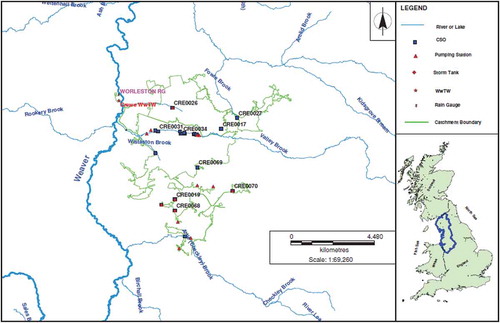
The Crewe catchment is located in the southeast Cheshire in the northwest of England (Fig. 1). The river system in the Crewe drainage area consists mainly of the River Weaver and its main tributaries Valley Brook and Wistaston Brook. The River Weaver itself lies just outside the drainage area boundary and receives direct discharge from Crewe Wastewater Treatment works. All CSOs in the study area discharge to Valley and Wistaston brooks, and to other smaller tributaries that eventually join the River Weaver.

Fig. 1 Crewe urban drainage area.

Daily rainfall data for the period 1960–2001 for Warleston raingauge in the Crewe catchment have been obtained from the Environment Agency for England and Wales. This rainfall time series has been used together with the corresponding climatic variables to build the downscaling model for rainfall in the catchment. Appropriate predictors for the rainfall in the catchment are selected from large-scale observed climatic variables via stepwise regression.

The large-scale observed climate data were obtained from the National Centers for Environmental Prediction (NCEP/NCAR). These observed data were used to calibrate and validate the downscaling model. The GCM data were obtained from the Canadian Climate Impacts Scenarios Group and the British Atmospheric Data Centre (BADC) with three different GCMs used for future projection of rainfall: the Hadley Centre Coupled Model version 3 (HadCM3), the Canadian Global Coupled Model version 2 (CGCM2) and the Commonwealth Scientific and Industrial Research Organization model (CSIRO Mark2).

3 Methodology

3.1 Downscaling model

A hybrid generalized linear model (GLM) and artificial neural network (ANN) approach (known hereafter as the GLM-ANN model), has been introduced in a previous study by the same authors (Abdellatif et al. 2011), and involved downscaling coarse GCM outputs to finer spatial scales.

The downscaling model developed used a two-stage process to model rainfall. The first stage is the rainfall occurrence process, which is modelled with logistic regression to represent wet and dry sequences of rainfall, and is given by equation (1), in which P_i is the probability of rain for the ith case in the dataset, x_i is a covariate vector (climate predictors) and β is a model coefficient (Chandler and Wheater 2002), as follows:

(1)

The second stage is the rainfall amount, which is modelled with a multi-layer feed-forward artificial neural network (MLF-ANN), described in equations (2) and (3), to represent the nonlinear relationship between the observed rainfall amount and the same selected set of climatic variables (predictors) used to model the rainfall occurrence process:

(2)

(3)

where y_i corresponds to the ith output (i.e. rainfall amount); x_i corresponds to the ith input (i.e. predictor set); the coefficients w_j⁽²⁾ and b⁽²⁾ (w_ij⁽¹⁾ and b_j⁽¹⁾) are the weights and biases from the output (hidden) layers; and f is the log-sigmoid transfer function.

The occurrence model is built first. This involves screening for appropriate predictors for the rainfall occurrence model. The screening process for rainfall predictors is achieved here by forming a stepwise regression between the rainfall series and the predictors. The predictors, which come from NCEP data, are then selected from a range of candidate predictors based on the significance and strength of their correlation with the predictand, as suggested by Wilby et al. (2004). Stepwise regression, also known as forward selection, is applied to the selection process as previous studies have shown that it yields the most powerful and parsimonious model (Huth 1999, Harpham and Wilby 2005). To remove any inconsistencies associated with the presence of small rainfall values, a threshold of 0.3 mm was applied to the data before modelling. Thus days with rainfall values less than this threshold are considered to be dry days and are represented by zero (Abdellatif et al. 2011), and those equal to or greater than the threshold are considered wet days and are represented by 1, to form a series of binary values for the occurrence of rainfall. The threshold treats trace rain days as dry days, as has been recommended in many studies (e.g. Wilby et al. 2003, Segond et al. 2006). Some transformations for the predictors have been applied, such as lag-1 or an exponential, to obtain the best correlation with the predictand.

Having selected the appropriate predictors, as explained above, the rainfall time series and selected predictor set were fitted to a generalized linear model (equation (1)) using logistic regression techniques. The fitted occurrence model was then used to resample the rainfall time series, ready for use in the second process of building the rainfall amount model.

The rainfall amount model is built using the selected predictors used in the occurrence model and the resampled rainfall. The MLF-ANN technique (equations (2)–(3)) is used to model the rainfall amount. The ANN model is trained using the Levenberg-Marquardt back-propagation algorithm.

The developed GLM-ANN model was then used to simulate annual future rainfall for corresponding wet days obtained from the occurrence model using a set of input variables generated by the GCMs (for a specific emissions scenario) as predictors.

To avoid the bias that may occur from using GCM variables to simulate future rainfall (2080s), correction for future rainfall (R_cf) is usually required. The correction proposed here consists of multiplying the future rainfall produced by the hybrid GLM-ANN model, R_{sim fut} for the A1FI and B1 scenarios with a ratio of the mean observed rainfall (Mean_ob) and the mean simulated rainfall (Mean_{sim.control run}) of the control period (1961–1990), as shown in equation (4). This method of correcting future rainfall is called the scaling (or direct) approach (Maraun et al. 2010), and can be expressed in mathematical terms as:

(4)

3.2 Temporal disaggregation of the downscaled rainfall

The small size and the rapid response of urban catchments, due to a high percentage of impermeable surfaces, require rainfall to be considered at small scales. This section describes the methodology of temporal rainfall disaggregation by applying the Bartlett-Lewis rectangular pulse (BLRP) stochastic model, employing the HYETOS programme (Koutsoyiannis and Onof 2000) for the purpose of disaggregating from daily to hourly rainfall. Moreover, the Poisson rectangular pulses model (PRP; Cowpertwait et al. 2004) in the STORMPAC 4.1 software (produced by WRc plc) is used to disaggregate the resultant hourly rainfall to 5 min.

3.2.1 Disaggregation from daily to hourly rainfall

The BLRP model assumes that the storm origins at a time (T) arrive according to the Poisson process with rate (λ) and the cell origins at a time (t) follow a Poisson process with rate (β), as depicted. The arrival of each storm is terminated after a particular time, and this length of time is exponentially distributed with parameter (γ). The distribution of the duration of the cells is an exponential distribution with parameter (η). The cell has uniform intensity or depth (X) with a specified distribution which can be either exponentially distributed with parameter 1/µ or can be chosen as a two-parameter gamma distribution with mean, µ_x and standard deviation, σ_x (Koutsoyiannis and Onof 2001). Thus, parameters β and γ also vary and are re-parameterized so that K = β/η and φ = γ/η.

The above description for the original BLRP model assumes that all parameters are constant; however, in the modified model, η varies randomly from one storm to another with a gamma distribution of shape parameter α and scale parameter ν.

The parameters for the BLRP are estimated on a monthly basis using the equations introduced by Rodriguez-Iturbe et al. (1988). The equations relate the statistical properties of the rainfall to the seven BLRP parameters, such as mean, variance, autocovariance and the proportion of dry days, which will result in a set of nonlinear equations. The equations of the BLRP model are solved using the method of moments, by equating the statistical feature of the historical rainfall with the theoretical one, using the approach of minimizing the sum of the weighted squared errors criteria.

The HYETOS software was used to disaggregate the daily rainfall at a single site into hourly data using fitted parameters. In HYETOS, the BLRP model was run several times until a sequence of exactly L wet days was generated (which is selected in the current study based on the maximum observed wet spell and should not exceed 12 days). Different sequences separated by at least one dry day can be assumed to be independent. Then, the intensities of all cells and storms are generated and the resulting daily depths are calculated. For each cluster of wet days, the generated synthetic daily depths should match the sequence of original daily totals with a tolerance distance, d defined as:

(5)

where N_i and Ñ_i are, respectively, the original and simulated daily totals at the raingauge station, with L the length of the sequence of wet days and C a small constant (=0.1 mm).

More detail on the calibration of the BLRP model and the fitted parameters can be found in Abdellatif et al. (2013). The outcome of this process is an hourly rainfall time series for the current and future period.

3.2.2 Disaggregation from hourly to 5-min rainfall

The methodology adopted here is similar to that used for disaggregating to an hourly scale in that ‘within-storm’ rain cells have arrival times that occur in a Poisson process. However, in the hourly approach, a Bartlett-Lewis model is used to disaggregate the daily data to hourly data, whilst in this approach, a simple Poisson process is used to simulate the fine-resolution (5-min) series directly from the hourly scale. This approach is just a special case of the Poisson rectangular pulse (PRP) model and is currently implemented in the STORMPAC 4.1 software.

In the PRP model, rain cells have arrival times (T) that occur in a Poisson process with rate λ. Each rain cell has a random lifetime (W), which is distributed as an independent exponential random variable with parameter η. The intensity (X) of each rain cell remains constant throughout the lifetime of the cell, and has been taken to be an independent Weibull random variable with parameters α and θ. The total rainfall intensity at any point in time is the sum of the intensities of all cells alive at that point (Cowpertwait 2005). Four parameters are used to construct the model: λ, η, α and θ, and need to be estimated (Fig. 2).

Fig. 2 Sketch of the Poisson rectangular pulse (PRP) model.

As in the BLRP, this model can be fitted by matching the above properties to their equivalent values taken from the sample, which can be achieved using a minimization procedure based on the squared differences; see Cowpertwait et al. (1991, 2004) for more information.

The disaggregation procedure used in STORMPAC 4.1 can be summarized as follows. A 1-h rainfall depth is read in from a file which contains the hourly series to be disaggregated. A 5-min series is simulated using the fitted model. The 5-min simulated series is summed and the 1-h total of the simulated series is compared to the 1-h total that was read in. The simulated series is discarded if the absolute difference between the simulated 1-h total and the total read in exceeds 0.05 mm. The process is repeated until the totals are in agreement to within 0.05 mm. The simulated series then represents a possible realization of 5-min data representative of the 1-h value that was read in.

Unlike HYETOS, which requires estimation of the model parameters at each different site prior to the disaggregation, the STORMPAC software does not. It is designed to be used for UK catchments and is supplied with parameters estimated from 99 rainfall sites across the UK used in the calibration of the model (more information about the model can be found in the STORMPAC 4.1 software manual).

3.3 Urban drainage modelling

The urban drainage area of Crewe is mainly served by a combined sewer system to handle its dry and wet weather flows. The catchment consists predominantly of residential housing interspersed with areas of retail, commercial and industrial developments, covering a total area of approximately 3363.33 ha, and serving a population of approximately 90 484. The sub-catchment runoff surface amounts to 2496.05 ha, with 16% impervious area and 83% pervious area. The sewer system in the study area is largely combined, although some areas of more recent development around the periphery of the town are drained by separate systems. The catchment sewer model consists of 1655 sub-catchments, 1830 nodes and 1797 sewers, with a total length of 94.64 km and sewer sizes ranging between 100 and 4500 mm.

The main receiving water within the Crewe drainage area is the River Weaver and its tributaries. The main river receives discharges from the Crewe Wastewater Treatment Works (WwTW), which is about 5 km northwest of Crewe town centre (United Utilities 2005). There are 23 CSOs within the catchment area (including CSOs and pump station emergency overflows, EOs) and one storm tank overflow, which all discharge into the tributaries of the River Weaver. The main focus of this study is spills from 19 critical CSOs in significant locations in the drainage areas, as shown in Fig. 1.

The model used has been built and verified by United Utilities Group PLC in northwest England. The model, which is built using the InfoWorks CS software developed by Innovyze Ltd, is permitted for academic use in this study. In order to use the model, it is required to determine the two main sources of flows in the urban area: the dry weather flow (DWF) and the design rainfall time series (DRTS).

3.3.1 Dry weather flow

The main constituents of the DWF are population-generated flows from residential properties within the network, and trade and commercial flows, together with infiltration from groundwater into the sewerage system.

For the purposes of this study, the Crewe sewer model used contains a population-generated flow of 128 l c^-1 d^-1 and a total trade and commercial flow of 20.16 and 28.75 L s^-1, respectively. An annual infiltration flow of 59.96 L s^-1 is used in the model.

3.3.2 Design rainfall time series

Continuous time series rainfall is required for assessment of the CSO discharge to account for any potential pollution to the receiving waters. Each of the 30 years of the present (1961–1990) and the future (2070–2099) hourly rainfall series is compared with its average annual and monthly rainfall in order to select the 10 most typical years, as specified in the United Utilities guidelines. The years are ranked in terms of the variance from the annual and monthly totals and from the average values for the baseline and future datasets. The series of 10 consecutive years from the 30 years with the lowest overall variance is then selected. The ranking systems were therefore set up in order to select the 10 years closest to the average year (TSRSim User Guide 2005). The selected 10-year rainfall series will be subjected to further analysis to select significant events based on selection criteria of 1.0-mm storm depth, 0.1-mm mean hourly rainfall intensity, 0.1-mm maximum intensity and an inter-event duration of 9 h, as per the United Utilities guidelines. These events are then disaggregated to 5 min using the STORMPAC software before being used in the model simulation.

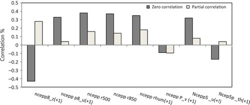
Fig. 3 Zero and partial correlation coefficients between rainfall occurrence and predictors.

For the purpose of the model simulation, the selected 10 years of rainfall need to be transformed into a surface runoff hydrograph with two principal parts. First, losses due to antecedent conditions (surface wetness and in-depth wetness of the catchment), areal reduction factor and evapotranspiration are deducted from the rainfall. Secondly, the resulting effective rainfall is transformed by surface routing into an overland flow hydrograph. In this process, the runoff moves across the surface of the sub-catchment to the nearest entry point to the sewerage system.

Surface wetness has been estimated using a linear regression model, and in-depth wetness is estimated using the rainfall and soil moisture deficit. Evaporation loss was calculated using a sinusoidal model, which is incorporated in the STORMPAC software.

For urban catchments in the UK, the percentage runoff coefficient can be estimated from the following models (Butler and Davies (2004):

1. Wallingford Procedure (fixed PR) runoff model:

The Wallingford model is applicable to typical urban catchments in the UK. It uses a regression equation to predict the runoff depending on the percentage of impermeability, the soil type and the antecedent wetness of each sub-catchment. The model predicts the total runoff from all surfaces in the sub-catchment, both pervious and impervious. Therefore this model should not be mixed with another model within one catchment. It is used to represent continuing losses with an initial loss model. In this model, runoff losses are assumed to be constant throughout a rainfall event and are defined by the relationship:

(6)

where PR is the percentage runoff; PIMP is the percentage impervious area (roads and roofs) by total contribution area; SOIL is an index of the water holding capacity of the soil; and UCWI is the urban catchment wetness index.

1. New UK (variable PR) runoff model:

This model is applicable to all catchments with all surface types, but particularly those which show significant delayed response from pervious areas. It calculates the runoff from paved and permeable surfaces separately and calculates the increase in runoff during an event as the catchment wetness increases. The percentage runoff is calculated using:

(7)

where IF is the effective impervious area factor; PF is the soil storage depth; and API30 is the 30-d antecedent precipitation index:

(8)

where N is the number of days prior to the event; (P– E)_n is the net rainfall on day n, with P_n the total rainfall depth and E_n the effective evaporation on day n; and C_p is the decay factor depending on the soil index.

4 Results and Discussion

4.1 Performance of the downscaling model

The first step in building a rainfall downscaling model for a catchment is the selection of predictors that may influence the occurrence and amount of rainfall in the catchment. Table 1 shows a list of eight appropriate predictors, together with their definitions, selected from a possible 18 candidates for rainfall occurrence at Worleston station. Figure 3 shows a bar chart of zero and partial correlation coefficients of the rainfall occurrence with the selected predictors. The coefficient ranges between 0.09 and 0.45 for zero correlation and between 0.04 and 0.28 for partial correlation. Despite the apparently low correlation coefficient, it was found that these relationships are statistically significant at a 5% level of significance. The selected predictors in Table 1 were then used to build a rainfall occurrence model for Worleston station using logistic regression (equation (1)). The observed data for the period 1961–1987 were used for model calibration, while 1988–2001 was used for model verification.

Table 1 Definitions of eight selected predictors (from the NCEP dataset).

Code	Variable
ncepp8_z(+1)	Lagged forward surface vorticity
ncepp p8_u(+1)	Lagged forward 850 hpa zonal velocity
ncepp r500	500 hpa Relative humidity
ncepp r850	850 hpa Relative humidity
ncepp rhum(+1)	Lagged forward near surface relative humidity
ncepp P_v (+1)	Lagged forward surface meridional velocity
ncepp5 _u(+!)	Lagged forward 500 hpa zonal velocity
ncep5 _th(+1)	Lagged forward 500 hpa wind direction

Table 2 presents measures for the accuracy of the rainfall occurrence model in terms of the percent correct (PC), Heidke skill scores (HSS) and bias, B (Wilks 1995). If HSS = 1, it means a perfect forecast, and if HSS = 0, it means that the model has no skill at all; however, if HSS < 0, the forecast is worse than a reference forecast (which normally should be the mean). Similarly, if B = 1, it means the forecast is unbiased; however, if B >1, it means there is an over-prediction, while B < 1 means there is an under-prediction. The PC usually ranges from zero, for no correct forecasts obtained by the model, to one, when all model forecasts are correct. Thus the results in Table 2 show that the model is capable of predicting rainfall occurrence with sufficient accuracy, as dictated by the higher values of PC (>75%) in both calibration and verification periods. The results indicate that the developed occurrence model is unbiased, with sufficient skills to predict occurrence of rainfall in the catchment.

Table 2 Percent correct (PC), Heidke skill scores (HSS) and bias (B) for the occurrence model.

Period	PC	HSS	B
Calibration	0.77	0.54	0.97
Verification	0.79	0.57	1.06
All	0.77	0.55	1.00

The rainfall amount model is then developed using the same predictors (Table 1), which are combined with the resampling scheme described above to form the rainfall artificial neural network model trained with the Levenberg-Marquardt back-propagation algorithm. Ninety percent of the observed daily rainfall in the period 1 January 1960 to 31 December 2001 is used for model calibration and the remaining 10% is used for model validation.

Five diagnostic tests are performed on the rainfall amount model to ensure its suitability for downscaling future rainfall in the catchment. These are demonstrated in Fig. 4 and Table 3. Figure 4(a) shows comparison plots of the average monthly rainfall amount between the observed and simulated rainfall series for the whole period 1961–2001. The plots demonstrate a good degree of agreement between the observed and simulated average monthly rainfalls, although the model tends to slightly overestimate the winter rainfall. It can be deduced from these plots that the model is able to reproduce the monthly rainfall. Figure 4(b) shows the inter-annual variability for the observed and simulated rainfall time series in the period 1961–2001. The monthly and yearly accumulations appear to have been reasonably captured by the model, which is an important requirement when assessing climate impacts on a hydrological system.

Fig. 4 (a) Observed and simulated average monthly rainfall. (b) Inter-annual observed and simulated rainfall. (c) Q-Q plot of observed and simulated rainfall. (d) Return period–return level relationship for the observed and simulated rainfall.

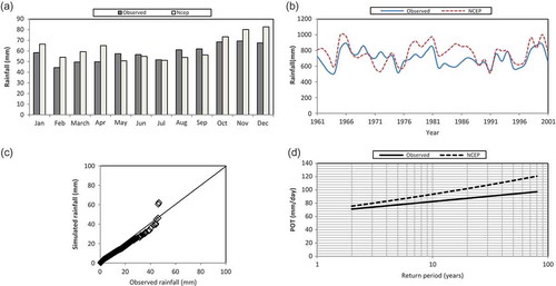
Table 3 Performance statistics of the rainfall amount model. RMSE: root mean square error; SD: standard deviation.

Method	RMSE	Correlation	Autocorrelation	SD
Observed rainfall			0.17	3.76
Simulated rainfall	3.14	0.68	0.31	1.8

The third diagnostic test is a plot of the quantiles of observed vs simulated rainfall values as presented in Fig. 4(c). It can be observed that the rainfall amount model results follow the 450 line, suggesting that the model is closer to the observed rainfall distribution. However, the model slightly underestimates the annual extreme rainfall. This closeness demonstrates further the capability of the model in reproducing the rainfall values.

The fourth diagnostic test is a plot for the return period–return level relationship between the observed and simulated daily rainfall, as depicted in Fig. 4(d). The combined peak-over-threshold generalized Pareto distribution approach was used to derive the relationship. A common threshold of 17 mm d^-1 was used for both rainfall series. The closeness of quantiles predicted by each rainfall series for the specified return period is a clear indication that the rainfall amount model is capable of reproducing the rainfall values.

The final diagnostic test is the statistics to evaluate the performance of the model, as presented in Table 3. The model shows better skill in predicting rainfall amount in terms of correlation and has a small root mean square error (RMSE). However, the model was not able to capture the autocorrelation and standard deviation statistics very well, which could be attributed to the intensive rainfall in the area which makes the rainfall highly skewed. The annual biases in autocorrelation and standard deviation of the simulated daily rainfall amounts are up to 78% and 52%, respectively, with respect to observed daily rainfall. This shows that the model is relatively conservative in reproducing the variability of daily rainfall (above 50%). Although the model would be more accurate if both the observed and simulated rainfall were closer to each other, with a low percentage error, the model is still able to capture rainfall variability, judging by the visual plots in Fig. 4, and the low RMSE and relatively high correlation coefficient values in Table 3.

Based on the outcomes of the diagnostic tests performed on the rainfall occurrence and amount models, the downscaling model developed for Worleston station can be considered reasonable for use in downscaling future rainfall in the Crewe catchment for the purpose of climate impact assessment.

4.2 Formation of the design rainfall time series

4.2.1 Selection of typical 10-year rainfall series

A typical 10-year rainfall time series is a sequence of rainfall events that is statistically representative of a rainfall pattern at a given location and is normally used for modelling spills from CSOs. The typical 10-year rainfall series will be used for testing the compliance of the CSO spills with the requirements for shellfish and bathing waters. Figure 5(a) represents an example for a validation check performed on the selected 10 years in ‘the 2080s’ for scenario A1FI from the HadCM3 GCM based on the average monthly rainfall depth. The plots in the figure ensure that the monthly variations in the selected 10 years of rainfall are sufficiently represented by the original 30 years of rainfall downscaled from the GCM. Figure 5(b) represents another check for consistency in the daily rainfall frequency in the two series for scenario A1FI of the HadCM3 GCM. The daily frequency plots in both figures demonstrate that the 10-year rainfall series is sufficiently representative of the rainfall in the Crewe catchment and can be used to model discharge from CSOs in the catchment. Statistically, the selected rainfall series is very similar to that generated by the downscaling model and the pattern of the rainfall distribution in the two series also matches well.

Fig. 5 (a) Average monthly rainfall depth in the 30-year and the typical 10-year rainfall series in 2080 from scenario A1FI of HadCM3. (b) Average daily rainfall frequency vs depth plots for the 30-year and the typical 10-year rainfall series in 2080 from scenario A1FI of HadCM3.

4.2.2 Pattern of future annual and bathing season rainfall

To investigate changes in the future annual and bathing-season (May–September in the UK) rainfall amounts, the annual and bathing-season rainfall from the selected typical 10-year series from each GCM and scenario were compared to the current conditions. Figure 6(a)  and (6b) presents plots for the annual and bathing-season rainfall, respectively. In Fig. 6(a), under scenario A1FI (high emissions), a similar increase in the annual rainfall is predicted by HadCM3 and CSIRO, whereas the prediction from CGCM2 shows a significant decrease in the annual rainfall. Under scenario B1 (low emissions) all GCM predictions indicate a decrease in annual rainfall. The bathing-season rainfall plots in Fig. 6(b) show that this is the only period in which all GCMs (under both scenarios) agree that there will be a decrease in rainfall, with a slight variation in the decreasing amount among the model predictions.

Fig. 6 (a) Future annual rainfall obtained from different GCMs for the high and low emissions scenarios. (b) Future bathing-season rainfall obtained from different GCMs for the high and low emissions scenarios. (c) Future number of rainfall events relative to the current conditions for the high and low emissions scenarios.

As climate change will affect rainfall frequency as well as magnitude, Fig. 6(c) shows a plot for the number of annual rainfall events predicted by the different GCMs under the high and low emissions scenarios relative to the current situation. It is clear from these plots that HADCM3 and CSIRO were found to predict the same number of events as in the current conditions under the high emissions scenario, whereas CGCM2 predicts a significantly smaller number of events. However, all the GCMs predict an increase in the number of events under the low emissions scenario, although rainfall is predicted to decrease under this scenario.

Figure 7 shows a plot for the average monthly rainfall residual, or difference between the predicted future rainfall from HadCM3 and the current conditions, for the 10-year rainfall series in the study catchment. Generally, rainfall intensities tend to decrease during the bathing season (May–September) and increase in the rest of the year, with significant increase associated with winter months (December, January and February), especially under the high emissions scenario.

Fig. 7 Monthly residual of rainfall for HadCM3 2080s.

4.3 Quantitative assessment of CSO spills

Nineteen CSOs in significant locations in the Crewe catchment were selected in the InfoWorks CS model of the catchment for assessment of their discharge into the receiving rivers. The 10 year rainfall series for the two scenarios produced by the three GCMs (six series), together with the base period (1961–1990), were analysed, as mentioned in Section 3.3.2, to form design rainfall time series before being used to simulate spills from CSOs in the Crewe catchment. Two sets of quantitative analysis were performed on the CSO simulation results using CSO spill drivers of spill volume, spill duration and spill frequency. One set of analysis was oriented to assess compliance of CSO spills to shellfish water requirements (a maximum limit of 10 spills per year); and the other set was oriented to assess compliance of CSO spills to bathing water requirements (a maximum limit of three spills per bathing season), as required by the Environment Agency for England and Wales (2009).

4.3.1 Assessment of CSO spills for shellfish water

Figure 8(a) to (c) shows the total spill volume, total spill duration and total spill frequency of the 19 CSOs, respectively, for the base and for the 2080s, as predicted by the three GCMs for scenarios A1FI and B, for shellfish water. The total spill from the CSOs, as projected by the HadCM3 and CSIRO GCMs, respectively, is predicted to increase under scenario A1FI with 37% and 6% for the spill volume, 32% and 2% for the spill duration, and 12% and 2% for the spill frequency. However, the same CSO spill drivers are predicted to decrease by the CGCM2 under the same scenario. Under scenario B1, all the GCMs agree on projecting a decrease in the three drivers from all CSOs where the percentage change between the GCMs ranged between 25 and 50% for spill volume, 21 and 39% for spill duration and 20 and 25% for spill frequency. The results from both scenarios reflect high uncertainty, which represents a significant difference between the GCM projections. This conflicting outcome is due to the inherent differences in the way that each GCM models the physics and chemistry of the upper atmospheric layers, in addition to the differences in grid resolution for each GCM.

Fig. 8 (a) Total spill volume, (b) total spill duration, and (c) total number of spills from the 19 CSOs per annum.

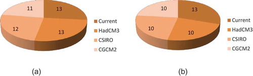
Figure 9(a) and (b) shows the number of CSOs in which the number of spills per year breaches the shellfish water spill limits for the current and future conditions under scenarios A1FI and B1, respectively. The number of CSOs breaching the spill limits is unchanged or decreases (from the current 13 CSOs) despite prediction of an increase in the number of spills under scenario A1FI. This is partly attributed to the prediction of significant reduction in rainfall during the summer (see Fig. 7). This would lead to a decrease in the number of spills in the summer, which in turn would affect the total number of spills per year. Under scenario B1, the number of CSOs breaching the spill limits is expected to decrease as rainfall is predicted to decrease by all the GCMs (see Fig. 6(a)).

Fig. 9 Number of unsatisfactory CSOs from 19 CSOs per annum for (a) A1FI and (b) B1 simulated by the three GCMs.

4.3.2 Assessment of CSO spills for bathing-season water

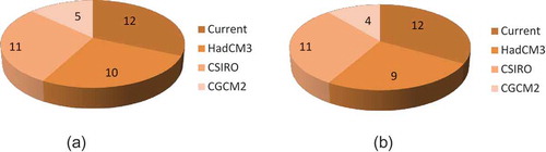
Figure 10(a) to (c) shows the total spill volume, total spill duration and total number of spills, respectively, from the 19 CSOs, for the base period and for the 2080s, as predicted by the three GCMs under scenarios A1FI and B for a bathing-water spill. The three drivers from the CSOs are projected to decrease by all three GCMs under both scenarios, with a significant decrease under scenario B1. This is because, among the scenarios considered, scenario A1FI has the highest concentration of atmospheric carbon dioxide (CO₂), while for B1 this concentration is decreased. The only exception here is for the results obtained from the CSIRO GCM, which projects change in the opposite direction, as there was a slight increase in the total number of spills from all 19 CSOs under scenario A1FI. The projected decrease in the three drivers of CSOs is clearly attributed to a significant reduction in rainfall predicted by all the GCMs (ranges between 45 and 70%) during this season, as illustrated in Fig. 6(b). Despite agreement of all GCMs on projecting the same pattern of climate change impacts on the drivers of CSO during this season, there are differences among the GCMs. For example, results from CGCM2 showed a substantial drop between 78 and 80% for spill volume, between 75 and 77% for spill duration and between 73 and 75% for spill frequency under both scenarios, while the results from HadCM3 and CSIRO projected a drop of 20 to 60% for spill volume, 0.7 to 49% for spill duration and 16 to 45% for spill frequency. The results also show a nonlinear relationship between the cause (storm) and the consequence (the three drivers of CSO spills) due to the dynamics of the system (distribution of the flow). The results further indicate that use of one GCM in an impact study is not enough to have a complete picture of what is going to happen in the future if uncertainty in the results is not highlighted.

According to the projection above, the number of CSOs which breach the bathing water spill limits is expected to decrease, as shown in Fig. 11(a) and (b).

Fig. 10 (a) Total spill volume, (b) total spill duration, and (c) total number of spills from the 19 CSOs per bathing season.

Fig. 11 Number of unsatisfactory CSOs from a total of 19 CSOs per bathing season for (a) A1FI and (b) B1 simulated by the GCMs.

5 CONCLUSIONS

The large urban drainage area of Crewe was used as a case study to demonstrate the use of downscaled rainfall time series to assess potential future pollution from spills of combined sewer overflows (CSOs). Seven typical 10-year design rainfall time series, representing present and future conditions derived from greenhouse-gas emission scenarios A1FI and B1, and the GCMs HadCM3, CSIRO and CGCM2 were used to simulate spills from the CSOs.

Although CSOs are used to help reduce urban flooding in combined sewerage systems, they can also be sources of pollution to the environment. The current paper provides a quantitative assessment of the CSOs under climate change conditions for the long-term future.

For 19 selected CSOs in the Crewe urban drainage catchment, the maximum annual projected increases are 37% increase in spill volume, 32% increase in spill duration and 12% increase in the number of rainfall events for the future conditions under the high emissions scenario. However, the system is expected to cope with climate change under the low emissions scenario, with annual reductions of up to 37%, 39% and 25%, respectively. Additionally, the analysis for the CSO spills for the future bathing season showed that, due to the prediction of a significant decrease in rainfall during this season, the total spill volume would reduce. However, pollution threat could increase due to low flows in the receiving water (to dilute pollutants) and high pollutant concentrations in the spill volume. Hence, this research should be of interest to all water companies in the UK, with a view to resolving expected future problems with their assets.

Disclosure statement

No potential conflict of interest was reported by the author(s).

Acknowledgements

This research was carried out at Liverpool John Moores University in collaboration with MWH UK Ltd and United Utilities. Special thanks from the authors go to Innovyse Ltd for providing an academic license for InfoWorks CS and to WRc for providing an academic license for STORMPAC. The views expressed in the paper are those of the authors and not necessarily those of the collaboration bodies.

REFERENCES

- Abdellatif, M., Atherton, W., and Alkhaddar, R., 2011. A methodology for downscaling rainfall in North West of England under climate change using hybrid GLM-ANN model. In: Proceeding 6th Annual BEAN conference, July 2012, Liverpool John Moores University, 142–149.
- Abdellatif, M., Atherton, W., and Alkhaddar, R., 2013. Application of the stochastic model for temporal rainfall disaggregation for hydrological studies in north western England. Journal of Hydroinformatics, 15 (2), 555–567. doi:10.2166/hydro.2012.090.
- Agency, E., 2009. Water quality planning: identifying schemes for the PR09 national environment programme. Bristol: Environment Agency.
- Andrew, F., 2008. Impact of climate change on frequency on pollution event, December. Shellfish Association of Great Britain Report.
- Busuioc1, A., et al., 2006. Comparison of regional climate model and statistical downscaling simulations of different winter precipitation change scenarios over Romania. Theoretical and Applied Climatology, 86 (1–4), 101–123. doi:10.1007/s00704-005-0210-8.
- Butler, D. and Davies, J., 2004. Urban drainage. New York: Spon Press.
- Chandler, R.E. and Wheater, H.S., 2002. Analysis of rainfall variability using generalized linear models – a case study from the West of Ireland. Water Resources Research, 38 (10), 1192.
- Cowpertwait, P.S.P. 2005. STORMPAC user guide. Report for WRc on Stochastic Disaggregation procedure Based on A Poisson Rectangular Pulses Model.
- Cowpertwait, P.S.P., Lockie, T., and Davies, M.D., 2004. A stochastic spatial-temporal disaggregation model for rainfall. Research Letters in the Information and Mathematical Sciences, 6, 109–123.
- Cowpertwait, P.S.P., et al., 1991. Stochastic generation of rainfall time series. Foundation for Water Research Report F0217.
- Fealy, R. and Sweeney, J., 2007. Statistical downscaling of precipitation for a selection of sites in Ireland employing a generalised linear modelling approach. International Journal of Climatology, 27 (15), 2083–2094. doi:10.1002/joc.1506.
- FitzGerald, A. 2008. Financial impacts of sporadic pollution events. Shellfish Association of Great Britain Report.
- Gamerith, V., et al., 2012. Assessment of combined sewer overflows under climate change—urban drainage pilot study Linz. In: IWA World congress on water, climate and energy, May 14–18, Dublin. IWA.
- Harpham, C. and Wilby, R.L., 2005. Multisite-Downscaling of heavy daily precipitation occurrence and amounts. Journal of Hydrology, 312, 235–255. doi:10.1016/j.jhydrol.2005.02.020.
- Haylock, M.R., et al., 2006. Downscaling heavy precipitation over the United Kingdom: a comparison of dynamical and statistical methods and their future scenarios. International Journal of Climatology, 21, 1923–1950.
- Hurcombe, P., 2001. Climate change and potential effects on sewerage systems. London: WaPUG Spring Meeting.
- Huth, R., 1999. Statistical downscaling in central Europe: evaluation of methods and potential predictors. Climate Research, 13, 91–101. doi:10.3354/cr013091.
- Keirle, R. and Hayes, C., 2007. A Review of climate change and its potential Impacts on water resources in the UK. E-WATER, June 2007 1–18.
- Kleidorfer, M., et al., 2009. A case independent approach on the impact of climate change effects on combined sewer system performance. Water Science and Technology, 60 (6), 1555–1564. doi:10.2166/wst.2009.520.
- Koutsoyiannis, D. and Onof, C. 2000. HYETOS a computer program for stochastic disaggregation of fine scale rainfall [online]. Available from: http://www.itia.ntua.gr/e/softinfo/3/ [Accessed 3 October 2013].
- Koutsoyiannis, D. and Onof, C., 2001. Rainfall disaggregation using adjusting procedures on a Poisson cluster model. Journal of Hydrology, 246 (1–4), 109–122. doi:10.1016/S0022-1694(01)00363-8.
- Maraun, D., et al., 2010. Precipitation downscaling under climate change: recent developments to bridge the gap between dynamical models and the end user. Reviews of Geophysics, 48 (3), RG3003.
- Nie, L., et al., 2009. Impacts of climate change on urban drainage systems – a case study in Fredrikstad, Norway. Urban Water Journal, 6 (4), 323–332. doi:10.1080/15730620802600924.
- Nilsen, V., et al., 2011. Analysing urban floods and combined sewer overflows in a changing climate. Journal of Water Climate Change, 2 (4), 260–271. doi:10.2166/wcc.2011.042.
- Ormsbee, L.E., 1989. Rainfall disaggregation model for continuous hydrologic modeling. Journal of Hydraulic Engineering, 115, 507–525. doi:10.1061/(ASCE)0733-9429(1989)115:4(507).
- Patz, J.A., et al., 2008. Climate change and waterborne disease risk in the Great Lakes region of the U.S. American Journal of Preventive Medicine, 35 (5), 451–458. doi:10.1016/j.amepre.2008.08.026.
- Rodriguez-Iturbe, I., Cox, D.R., and Isham, V., 1988. A point process model for rainfall: further developments. Proceedings of the Royal Society A: Mathematical, Physical and Engineering Sciences, 417, 283–298. doi:10.1098/rspa.1988.0061.
- Segond, M.L., Onof, C., and Wheater, H.S., 2006. Spatial-temporal disaggregation of daily rainfall from a generalized linear model. Journal of Hydrology, 331, 674–689. doi:10.1016/j.jhydrol.2006.06.019.
- Tait, S.J., et al., 2008. Sewer system operation into the 21st century, study of selected responses from a UK perspective. Urban Water Journal, 5 (1), 79–88. doi:10.1080/15730620701737470.
- Titterington, J.A., 2008. Advanced wastewater modelling. Warrington: Unpublished training notes for MWH modellers.
- TSRSim, 2005. User Guide. Wallingford: HR Wallingford.
- United Utilities, 2005. Douglas UID Study. Report no. RT-NW-2677-02.
- Vasiliades, L., Loukas, A., and Patsonas, G., 2009. Evaluation of a statistical downscaling procedure for the estimation of climate change impacts on droughts. Natural Hazards Earth System Science, 9, 879–894. doi:10.5194/nhess-9-879-2009.
- Wilby, R.L., Tomlinson, O.L., and Dawson, C.W., 2003. Multi-site simulation of precipitation by conditional resampling. Climate Research, 23, 183–194. doi:10.3354/cr023183.
- Wilby, R.L., et al., 2004. The guidelines for use of climate scenarios developed from statistical downscaling methods [online]. Supporting material of the Intergovernmental Panel on Climate Change (IPCC). UK. Available from: http://ipcc-ddc.cru.uea.ac.uk/ [Accessed 30 August 2013].
- Wilks, D., 1995. Statistical methods in atmospheric sciences. London: Academic Press.