Modelling climate and land-use change impacts with SWIM: lessons learnt from multiple applications

Abstract

The Soil and Water Integrated Model (SWIM) is a continuous-time semi-distributed ecohydrological model, integrating hydrological processes, vegetation, nutrients and erosion. It was developed for impact assessment at the river basin scale. SWIM is coupled to GIS and has modest data requirements. During the last decade SWIM was extensively tested in mesoscale and large catchments for hydrological processes (discharge, groundwater), nutrients, extreme events (floods and low flows), crop yield and erosion. Several modules were developed further (wetlands and snow dynamics) or introduced (glaciers, reservoirs). After validation, SWIM can be applied for impact assessment. Four exemplary studies are presented here, and several questions important to the impact modelling community are discussed. For which processes and areas can the model be used? Where are the limits in model application? How to apply the model in data-poor situations or in ungauged basins? How to use the model in basins subject to strong anthropogenic pressure?

Editor D. Koutsoyiannis; Associate editor C. Perrin

Résumé

Le modèle intégré eau et sol (Soil and Water Integrated Model (SWIM) est un modèle écohydrologique semi-distribué continu, intégrant les processus hydrologiques, la végétation, les nutriments et l’érosion. Il a été développé pour l’évaluation d’impacts à l’échelle du bassin versant. SWIM est couplé à un SIG et a des besoins modestes en données. Au cours de la dernière décennie, SWIM a été largement testé sur des bassins de tailles intermédiaires et grandes, au niveau des processus hydrologiques (débit, eau souterraine, évapotranspiration), de la dynamique des nutriments, des événements extrêmes (crue et étiage), du rendement des cultures, et de l’érosion. Plusieurs modules ont été développés de manière plus approfondie (zones humides et dynamique de la neige) ou introduits (glaciers, réservoirs). Après validation, SWIM peut être appliqué pour des évaluations d’impacts. Nous présentons ici quatre exemples d’études, discutons de plusieurs questions importantes pour les modélisateurs s’intéressant aux impacts. Pour quels processus et surfaces le modèle peut-il être utilisé ? Comment appliquer le modèle dans des situations de faible disponibilité en données ou sur des bassins non jaugés ? Comment utiliser le modèle dans des bassins sujets à de fortes pressions d’origine humaine ?

Key words:

• ecohydrological model
• river basin
• climate change impact
• land-use change impact
• calibration and validation
• process-based model

Mots clefs:

• modèle écohydrologique
• bassin versant
• impact des changements climatiques
• impact des changements d’occupation des sols
• calage et validation
• modèle orienté processus

1 INTRODUCTION: PROCESS-BASED MODELS FOR RIVER BASINS AS TOOLS FOR IMPACT ASSESSMENT

Regional-scale hydrological models can play an important role in river basin management. They simulate impacts and effects of possible future changes and help to find measures for improving the adaptive capacity of river basins. Several types of hydrological models for river basins are distinguished. Two important criteria for the model classification are their physical basis and spatial structure.

The continuous dynamic models of intermediate complexity that include mathematical descriptions of physical, biogeochemical and hydrochemical processes, and combine equations of both physical and conceptual semi-empirical nature are called process-based models. They are usually semi-distributed and apply two- or three-level disaggregation schemes, e.g. in sub-basins and hydrotopes or Hydrologic Response Units (HRU), based on the overlaying of sub-basins, land-use and soil maps. Numerous studies have demonstrated that such models are able to adequately represent natural processes at the catchment scale.

A process-based ecohydrological model for a river basin inevitably contains a hydrological module as a basic element. Other necessary components are: a vegetation submodel and, usually, modules for biogeochemical cycles (carbon, C, nitrogen, N, and phosphorus, P). The hydrological, vegetation and biogeochemical submodels are usually coupled in order to include important interactions and feedbacks between the processes, such as water and nutrient drivers for plant growth, water transpiration by plants, nutrient transport with water etc. Usually, vertical and lateral fluxes of water and nutrients are modelled separately, whereas climate parameters are used as external drivers.

The Soil and Water Integrated Model (SWIM) (Krysanova et al. 1998, 2000) belongs to the process-based modelling tools. In comparison with other hydrological models, SWIM is a model of intermediate complexity: being more complex than HBV (Bergström 1995) and TOPMODEL (Beven and Kirby 1979), and simpler than a fully distributed model, such as MIKE SHE (Abbott et al. 1986).

The SWIM is based on two previously developed tools—SWAT (Arnold et al. 1993), and MATSALU (Krysanova et al. 1989). SWAT is a hydrological model widely used for assessment of agricultural and water management practices worldwide, as well as for impact studies. The other model, MATSALU, was developed in Estonia for the agricultural basin of the Matsalu Bay (3500 km²) and the bay ecosystem in order to evaluate several management scenarios for eutrophication control. Both predecessors, SWAT and MATSALU drew from the CREAMS model (Knisel 1980). Besides, SWAT is partly based on the EPIC approach (Williams et al. 1984), and later the APEX model was developed (Williams et al. 1995, Gassman et al. 2010) to simulate a wide array of management practices across a broad range of agricultural landscapes, and to bridge the gap between SWAT and EPIC.

Both models SWAT and SWIM have many similar process descriptions and some differences (see Krysanova et al. 2005), and both are being developed further. The history of the SWAT and SWIM development is presented in Krysanova and Arnold (2008). The further development of SWIM follows the needs of its main application for climate and land-use change impact assessments, and the spatial scale of typical applications (basins with drainage areas varying from 1000 to 200 000 km² and larger). Therefore, specific processes are included or extended, such as snow and glacier dynamics, wetlands, CO₂ fertilization effects on plant physiology and reservoir water storage.

The objectives of this paper are: (a) to present an overview of processes represented in SWIM and how the model was tested for them; (b) to show and discuss a number of impact assessments performed with the model; and (c) based on experience of model application, to discuss lessons learnt and questions of importance to modellers, e.g. the limits of model applicability in close-to-natural and managed catchments, the methodology of impact assessment, etc. This can be useful for modellers applying hydrological and ecohydrological models for water resources assessment and impact studies.

After a short description of the model in Section 2, several SWIM applications are presented in Section 3, showing model performance for simulating hydrological processes, including extremes, erosion, water quality, groundwater dynamics and wetlands, crop yield, snow dynamics, reservoirs and inundation processes. Several climate and land-use change impact studies are presented in Section 4, and the lessons learnt are summarized in Section 5.

2 SHORT DESCRIPTION OF THE MODEL

The ecohydrological model SWIM (Fig. 1) is a continuous-time, spatially semi-distributed model, integrating hydrological processes, vegetation growth (agricultural crops and natural vegetation), nutrient cycling (C, N and P), and sediment transport at the river basin scale. More detailed information on the model can be found in Krysanova et al. (2000).

Fig. 1 SWIM structure.

2.1 Hydrological system

The simulated hydrological system consists of four control volumes: the soil surface, the root zone of soil (subdivided into several layers), the shallow aquifer and the deep aquifer. The water balance for the soil surface and soil column includes precipitation, surface runoff, evapotranspiration, subsurface flow and percolation. The water balance for the shallow aquifer includes groundwater recharge, capillary rise to the soil profile, lateral flow, and percolation to the deep aquifer.

Surface runoff is estimated as a nonlinear function of precipitation and a retention coefficient, which depends on the soil water content, land use and soil type (modification of the curve number method, Arnold et al. 1990). The method was adapted to German conditions by validation in seven mesoscale catchments with different climatic conditions, land use and soils. Lateral subsurface flow is calculated simultaneously with percolation. It occurs if the storage in any soil layer exceeds field capacity after percolation and is especially important for soils with an impermeable or less permeable layer below several permeable ones. Potential evapotranspiration is estimated using the method of Priestley-Taylor (Priestley and Taylor 1972), though the method of Penman-Monteith (Monteith 1965) can also be used. Actual evaporation from soil and actual transpiration by plants are calculated separately.

2.2 Crops and natural vegetation

This module is an important interface between hydrological processes and nutrients. Plant growth is mainly driven by solar radiation and main plant stress factors, such as water availability and temperature. A simplified EPIC approach (Williams et al. 1984) is included in SWIM for simulating arable crops (e.g. wheat, barley, rye, maize, potatoes) and aggregated vegetation types (such as ‘pasture’, ‘evergreen forest’, ‘mixed forest’), using specific parameter values for each crop/vegetation type. Numerous plant-related parameters are specified for 74 crop/vegetation types in the database attached to the model. Vegetation in the model affects the hydrological cycle by the cover-specific retention coefficient, impacting on surface runoff, and indirectly influencing the amount of transpiration, being a function of potential evapotranspiration and leaf area index (LAI).

Interception of photosynthetic active radiation (PAR) is estimated as a function of solar radiation and LAI. The potential increase in biomass is the product of absorbed PAR and a specific plant parameter for converting energy into biomass. The potential biomass is adjusted daily with the help of plant stress factors. The LAI is simulated as a function of a heat unit index (ranging from 0 at planting to 1 at physiological maturity) and biomass.

2.3 Sediment yield

Sediment yield is calculated with the Modified Universal Soil Loss Equation (MUSLE, Williams and Berndt 1977) using the surface runoff, the peak runoff rate, the soil erodibility factor, the crop management factor, the erosion control practice factor, and the slope length and steepness factor for every hydrotope inside the sub-basin. The sediment routing model consists of two components operating simultaneously—deposition and degradation in the streams, both dependent on stream velocity.

2.4 Nitrogen and phosphorus modules

These modules include the following pools in the soil layers (Fig. 1): nitrate and ammonium nitrogen (NO₃-N, NH₄-N), active (N_o-ac) and stable (N_o-st) organic nitrogen, organic nitrogen in the plant residue (N_res), labile phosphorus (P_lab), active (P_m-ac) and stable (P_m-st) mineral phosphorus, organic phosphorus (P_org), and phosphorus in the plant residue (P_res), and the following fluxes: fertilization, input with precipitation, mineralization, denitrification, plant uptake, leaching into groundwater, losses with surface runoff, interflow and erosion. The interaction between vegetation and nutrient supply is modelled by the plant uptake of nutrients, release of residuals entering mineralization process, and by using N and P stress factors, which affect plant growth.

2.5 Recently developed modules

For more than a decade, many SWIM modules have been tested and enhanced, and several new modules have been added. The new modules are: Muskingum routing method, CO₂ fertilization, crop rotation generator (several versions), nutrient retention, wetland module (two versions), C cycle, dynamical forest module, in-stream nutrient processes, inundation module, glacier module, reservoirs and irrigation water use. Other components, such as the snow module, were enhanced by including additional processes. However, the C cycle, the dynamical forest module, the inundation module and the detailed wetland module represent special model versions, and are not included in the standard version of SWIM. The in-stream nutrient processes and the reservoir module are on the way to being included in the standard version of SWIM.

2.6 Data to operate SWIM

Input data needed to drive the model include: digital elevation model (DEM), land-use map, soil map and parameterization of soil layers (texture, porosity, available water capacity, field capacity, saturated conductivity, C and N content and erodibility), climate data (daily minimum, maximum and average temperature, precipitation, air humidity and solar radiation) and management data (crops, fertilization, water management, point sources, etc.). Besides, water discharge and water quality data are needed for the model calibration. Most of these data are usually available in regional or global datasets, and missing parameters could be estimated. However, water quality data are not always available (especially in developing countries), and sampling frequency may be not satisfactory.

2.7 GIS interfaces

SWIM includes the interfaces to the geographic information system GRASS (http://grass.osgeo.org/documentation/manuals/; Neteler and Mitasova 2008) and MapWindow (http://www.mapwindow.org/), both serve to the extraction of spatially distributed parameters of elevation, land use, soil, vegetation, hydrotope structure and the creation of the routing structure for the basin under study. A climate interpolation module is included in the MapWindow interface, but performed separately when the GRASS interface is used. Climate parameters are interpolated to the centroids of every sub-basin using the inverse distance or kriging method, taking into account elevation. In contrast to the GRASS interface, the MapWindow interface is more user-friendly and it also includes some basic post-processing (visualization of results).

2.8 Dissemination of the model

The dissemination of the model is restricted to project partners (e.g. common EU projects), other collaboration partners and experienced modellers, primarily because it is not possible to provide day-to-day modelling support for numerous inexperienced users. In such cases, the requests are responded with an advice to use the similar model, SWAT, which is available for download as a public domain tool, and is supported daily by the SWAT team in Temple and College Station, Texas, USA.

3 DIVERSITY OF SWIM APPLICATIONS

SWIM calibration and validation was performed at the river basin scale, not only for hydrological processes, but also for extreme events, water quality, crop yield, etc. In most cases, but not always, the validation results were satisfactory. The problems encountered in the model calibration often led to improvement of process description and model modification. The most thorough validation has been done for catchments in Germany, and during the last years it has been extended also to other EU countries and to river basins in Africa, Asia, and South America. Table 1 shows an overview of the most important SWIM applications with references. This section presents examples of SWIM validation studies for different components, and discusses problems encountered and lessons learnt. The studies were selected with the aim of showing the model testing for different processes based on the recent results.

Table 1 Overview of the most important applications of SWIM.

Processes modelled	Catchment(s)/Region	References
Hydrology (mesoscale)	Five sub-basins of the Elbe	Krysanova et al. (1998), Krysanova et al. (1999)
Hydrology (large scale)	Elbe; Five river basins in Germany	Hattermann et al. (2005); Huang et al. (2010)
Water quality (mesoscale)	Stepenitz (Elbe); Rhin (Elbe)	Krysanova et al. (1998), Krysanova and Becker (1999); Hesse et al. (2008)
Water quality (large scale)	Saale (Elbe)	Krysanova and Haberlandt (2002), Huang et al. (2009), Hesse et al. (2012, 2013)
Groundwater	Nuthe and Stepenitz (Elbe)	Hattermann et al. (2004)
Snow and glaciers	Upper Rhine and Upper Danube; Aksu (Tarim*)	Huang et al. (2013b); Wortmann et al. (2013)
Inundation	Niger (Africa)	Liersch et al., (2012a, 2012b)
Irrigation	Aksu (Tarim*)	Huang et al. (2015)
Reservoirs	Niger (Africa)	Koch et al. (2013)
Wetlands	Nuthe (Elbe)	Hattermann et al. (2006, 2008)
Soil moisture	Brandenburg (Germany)	Holsten et al. (2009)
Erosion	Mulde (Elbe); Glonn (Isar, Danube)	Krysanova et al. (1998); Krysanova et al. (2002)
Crop yield	Brandenburg (Germany); Elbe; Field plots in Brandenburg	Krysanova et al. (1998, 1999, 2007); Post et al. (2007)
Forest dynamics	Brandenburg (Germany)	Wattenbach et al. (2005)
Climate change impact on water	Brandenburg, Germany; Five river basins in Germany; Niger, Blue Nile, Limpopo, Oubangui (Africa); Rhine (Europe), Upper Niger (Africa), Upper Yellow (China)	Krysanova et al. (1999); Huang et al. (2010), Hattermann et al. (2011); Aich et al. (2014); Vetter et al. (2014)
Climate change impact on floods	Five river basins in Germany	Huang et al. (2013a), Hattermann et al. (2012)
Climate change impact on low flow	Five river basins in Germany	Huang et al. (2013b)
Climate change impact on crop yield	Brandenburg (Germany); Ems and Elbe (Germany)	Krysanova et al. (1999); Huang et al. (2012)
Climate change impacts on carbon dynamics	Sub-basins of the Elbe; Elbe	Post et al. (2008a); Post et al. (2008b)
Land-use change impact on water	Brandenburg, Germany; Rhin and Saale (Elbe)	Wechsung et al. (2000); Hesse et al. (2008, 2012)
Land-use change impact on water quality	Rhin and Saale (Elbe); Weiße Elster (Elbe)	Hesse et al. (2008, 2012); Boyacioglu et al. (2011)

*Kyrgyzstan and China

3.1 Hydrological processes

Extensive calibration and validation of SWIM was performed in the framework of climate impact assessment for Germany (see more details and input data description in Huang et al. 2010, 2013a, 2013b, Hattermann et al. 2011). It was done for the five largest river basins in Germany: the Danube, Elbe, Ems, Rhine, Weser, and their tributaries, covering 90% of the whole German territory. The model was calibrated and validated for the last gauges, for intermediate gauges with drainage area larger than 5000 km² and also for few gauges with drainage areas smaller than 5000 km². The major parameters used for the calibration are listed in Table 2.

Table 2 List of major parameters used for hydrological calibration of SWIM.

Parameter	Description	Range
abf	Alpha factor of groundwater which characterizes the groundwater recession (the rate at which groundwater flow is reaching stream)	0.01–6.0
bff	Baseflow factor for basin, which characterizes water percolation in soil profile from layer to layer	0.2–1.0
del	Groundwater delay (days): time needed for water leaving the bottom of the root zone to reach the shallow aquifer	10–200
gwq0	Initial groundwater flow contribution to streamflow (mm/d)	0.01–6.0
roc2	Routing coefficient to calculate the storage time constant for the reach (surface layer)	1–20
roc4	Routing coefficient to calculate the storage time constant for the reach (subsurface layer)	1–20
sccor	Correction factor for saturated conductivity (applied for all soils)	0.01–10.
thc	Correction factor for potential evapotranspiration on sky emissivity	0.3–1.5

Table 3 shows the Nash-Sutcliffe (Nash and Sutcliffe 1970) efficiency (NSE) and the logarithmic Nash-Sutcliffe efficiency (LNSE) criteria in the respective calibration and validation periods, 1961–1980 and 1981–2000. As is evident, SWIM reproduces the river discharges in most German rivers adequately. In general, obtaining values of NSE and LNSE greater than 0.7 is considered as satisfactory for hydrological simulation, and some authors suggest even lower threshold values (e.g. 0.54–0.65 is treated by Moriasi et al. (2007) as ‘good’, and >0.65 as ‘very good’ for daily hydrological modelling). The guideline criteria to assess the adequacy of simulated discharge were also provided by Chiew and McMahon (1993). As shown in Table 3, the NSE and LNSE values are higher than 0.7 for 75% and 80% of gauges, respectively, in the calibration period, and for 67% of gauges in the validation period. Besides, SWIM was also tested for reproduction of other hydrological variables such as soil moisture (Holsten et al. 2009) and groundwater level (Hattermann et al. 2004).

Table 3 Nash-Sutcliffe (Nash and Sutcliffe 1970) efficiency (NSE) and logarithmic Nash-Sutcliffe efficiency (LNSE) for the calibration and validation periods for the selected gauges (see full version in Huang et al. 2013b).

River basin	Rivers	Gauges	Area (km^2)	NSE		LNSE
				Calibration 1961–1980	Validation 1981–2000	Calibration 1961–1980	Validation 1981–2000
Ems	Ems	Versen	8 369	0.80	0.86	0.79	0.79
	Ems	Dalum^1	4 981	0.80	0.85	0.78	0.72
Weser	Weser	Intschede	37 720	0.90	0.90	0.88	0.86
	Weser	Vlotho^1	17 618	0.84	0.87	0.80	0.85
	Aller	Marklendorf	7 209	0.74	0.60	0.72	0.63
	Leine	Schwarmstedt	6 443	0.82	0.74	0.86	0.82
	Fulda	Guntershausen^1	6 366	0.73	0.75	0.65	0.70
Danube	Danube	Achleiten ^1	76 653	0.86	0.85	0.86	0.85
	Danube	Hofkirchen	47 496	0.84	0.85	0.85	0.84
	Danube	Pfelling^1	37 687	0.80	0.81	0.83	0.80
	Inn	Passau Ingling	26 084	0.83	0.80	0.85	0.83
	Danube	Donauwoerth ^1	15 037	0.77	0.78	0.79	0.79
Rhine	Rhine	Rees^1	159 300	0.84	0.85	0.84	0.82
	Rhine	Andernach^1	139 549	0.83	0.81	0.83	0.78
	Rhine	Maxau^1	50 196	0.66	0.67	0.71	0.68
	Rhine	Rheinfelden	34 550	0.68	0.71	0.71	0.71
	Main	Frankfurt-Osthafen	24 764	0.72	0.81	0.82	0.81
	Moselle	Trier Up	23 857	0.86	0.84	0.87	0.88
	Neckar	Rockenau SKA	12 710	0.78	0.80	0.84	0.83
Elbe	Elbe	Neu-Darchau	131 950	0.84	0.79	0.84	0.76
	Elbe	Dresden^1	53 096	0.70	0.70	0.70	0.63
	Elbe	Schöna^2	51 391	0.64	0.61	0.58	0.61
	Havel	Havelberg^2	24 037	0.42	0.64	0.16	0.55
	Saale	Calbe-Grizehne	23 719	0.78	0.57	0.78	0.66
	Mulde	Bad Dueben	6 171	0.73	0.71	0.81	0.80

¹ Gauges not calibrated.

² Observed discharge is only available for 1975–1992 for Schöna and 1981–1995 for Havelberg, so the calibration period is the first half of the period.

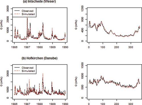
Figure 2 provides two examples of the comparison between the simulated and observed river discharge in the Weser and the Danube as the daily time series in the period 1986–1989 (Fig. 2, left), and as average daily dynamics in the same period (Fig. 2, right). These two examples represent two hydrological regimes in Germany: the pluvial regime (Weser) with high flows in winter and low flows in summer and the pluvio-nival regime (Danube) with high flows in both winter and early summer. In both examples the simulated river discharge is in good agreement with the observed one, and the seasonal dynamics is also well reproduced. This illustrates the suitability of SWIM for modelling hydrological processes in large regions with different hydrological conditions.

Fig. 2 Simulated and observed water discharge (left) at the gauges (a) Intschede (Weser) and (b) Hofkirchen (Danube) in the calibration period 1986–1989, and the corresponding average daily discharge (right) for the same stations in the same period (see an extended version in Huang et al. 2010). The corresponding NSE values for (a) and (b) are 0.92 and 0.90, respectively.

There are only a few ‘problematic’ gauges (e.g. Havelberg) where simulated results do not comply with the observed values well enough. This is mainly due to large-scale human interventions, which could not be reproduced in the model due to poor data sources in these cases. For example, in the Havel River basin, large amounts of groundwater were abstracted and discharged into rivers before 1990 due to the large-scale open-pit mining operations in the Lusatia (Grünewald 2001). This substantial influence on the hydrological cycle was not considered by the model, but affected the results of model calibration.

In a separate study, Conradt et al. (2012) used the naturalized discharge data, i.e. when effects of water management and mine discharges were removed from the measured discharge, to calibrate and validate SWIM for the Elbe River basin, including the Havel sub-basin. However, this ‘naturalization’ is very time- and data-consuming and therefore is often not possible.

3.1.1 Failure cases

Our experience of hydrological calibration using SWIM shows that anthropogenic water management in watersheds not supported by data is the main problem preventing satisfactory model calibration in mesoscale and large river basins. The most extreme case until now was in China, in the densely-populated Yongding River basin (about 47 016 km²), with very intensive water use and management (see http://www.guanting.de), where the SWIM application without information on reservoir management and irrigation could not simulate a hydrograph comparable to the observed one. The other problematic case is attributable to simulating river discharge for small-scale catchments (<100 km²), being more sensitive to human interferences (Huang et al. 2013b) and input data quality, such as location of climate/precipitation stations, soil parameterization and land use.

3.1.2 Lessons learnt

Spatial discretization of a basin under study in sub-basins of reasonable size (Krysanova et al. 2000), availability of precipitation data with sufficient density (e.g. one station per 100 km², depending on topography), interpolation of climate data to sub-basins instead of simply using the nearest stations, as well as reasonable parameterization of soils, are important for obtaining good calibration and validation results. The multivariate (discharge, groundwater, vegetation) and multi-site validation improves reliability of results, especially if different processes are studied. A possible option for increasing the credibility of results is a comprehensive validation including quantification of uncertainty.

In general, different approaches can be applied for hydrological modelling in river basins with human interventions: either ignoring them (if small or not important to the research question), or including them in the model (e.g. reservoirs or irrigation activities), or using the naturalized discharge data for model calibration.

3.2 High and low flows

The SWIM has also been applied for the modelling of extreme hydrological events: high flows and low flows under climate change in Germany, and the model was tested for reproducing extreme conditions and calibrated/validated for them in advance.

The modelling of floods was focused on the high flows (95th and 99th percentile discharges), flood events (with a 10- or 30-year return period) and large flood events (50-year return period). For the characterization of low-flow conditions, two parameters were used: (a) the annual minimum 7-day mean flow, and (b) the stream deficit volume (a cumulative deficit of streamflow below 90% exceedence frequency of the flow duration curve) that are widely used to describe the low-flow and drought conditions. The model was calibrated and validated for extremes in 30 gauge stations located at the main rivers and their large tributaries.

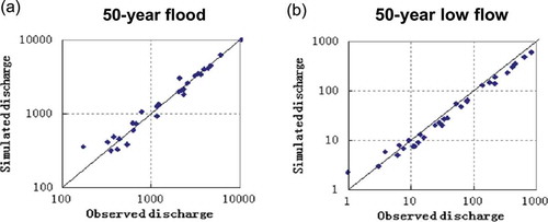
Figure 3 summarizes the results for 50-year flood and low-flow levels at the 29 gauges estimated for the period 1961–2000 versus the corresponding observed values. It can be seen that the extreme flood level can be well simulated by SWIM but most low flows are marginally underestimated. This underestimation may be partly due to regulation of low-flow regimes using storage reservoirs that were not considered in the hydrological modelling.

Fig. 3 Comparison of the simulated 50-year flood and low-flow levels at 29 gauges in Germany with the observed ones for the period 1961–2000.

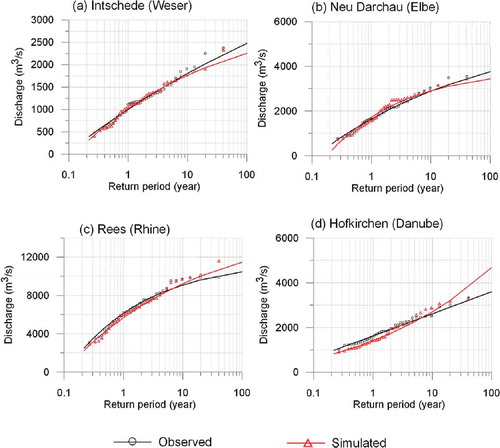
Some examples of flood frequency plots created by fitting the observed and simulated (using observed climate data) annual maximum daily discharge with the generalized extreme value distribution (GEV; Coles 2001) for 1961–2000 are shown in Fig. 4. In general, the GEV fitting curves for the observed values are well comparable with those for the simulated values. However, for the gauge Hofkirchen (Danube), there is a relatively large bias for the extreme flood events.

Fig. 4 Generalized extreme value (GEV) plots for the annual maxima of observed daily discharge and simulated discharge using observed climate data of 1961–2000 for four selected gauges in Germany; their drainage areas are indicated in Table 2.

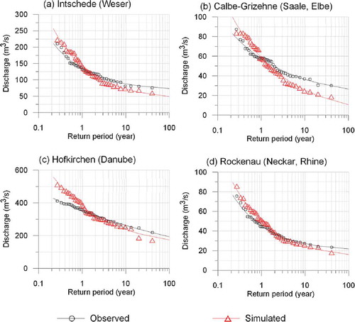
Figure 5 includes four examples, demonstrating that SWIM driven by the observed climate data can reproduce the low-flow frequency curves reasonably well. It is interesting to observe that the low-flow levels of return periods lower than 1 year are slightly overestimated, while those of return period larger than 10 years are underestimated. These disagreements may be partly systematic (also related to the choice of estimation method) and partly due to the anthropogenic modifications of low-flow regimes which were not accounted for in the model. In addition, the ‘static’ land-use information used in the whole modelling period may also contribute to a bias of the simulation results.

Fig. 5 Return level plots for the observed and simulated annual minimum 7-day discharge (AM7) at four selected gauges in Germany in the period 1961–2000; their drainage areas are indicated in Table 2.

We can conclude that SWIM can successfully reproduce river discharges and extremes using observed climate data in most of the studied gauges in Germany. The results of calibration and validation for extreme conditions are described in detail in Huang et al. (2013a, 2013b).

3.2.1 Lessons learnt

For the estimation of return periods of extremes, the reference period should be as long as possible. In general, local human interferences, such as land-use change and hydraulic structures, may have important impacts on river low flow in addition to the climate driver (and in some cases could have even greater influence on the discharge than climate change), especially for small rivers. Therefore, human influences may be neglected only for cases where such impacts are small. However, for the impact assessment, when the ‘pure’ impact of warmer climate is of interest, the validation results as presented in Figs 3–5 are sufficient, and the human interferences may be ignored.

3.3 Erosion

Though SWIM has been rarely used for simulation of erosion processes in the past, it is planned to include these processes in the impact studies in the future. Here we briefly illustrate the applicability of the model for simulation of sediment transport.

The SWIM was tested for its ability to simulate sediment yield and transport at the catchment scale (Krysanova et al. 2002) by applying it to the Glonn (392 km²) and the Mulde (6171 km²) river basins in Germany, in order to (a) validate basin-scale sediment transport modelling; (b) investigate scaling issues; and (c) study the linkage between hydrological processes and sediment yield and transport in the model. Daily water discharge and suspended sediment data available for the gauge Hohenkammer for 15 years were used for the model calibration and validation.

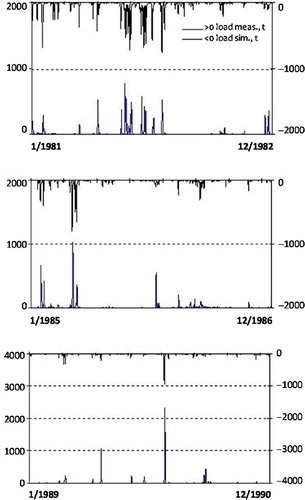
Some results of sediment load modelling with SWIM are presented in Fig. 6, which depicts daily dynamics of simulated and measured suspended sediment loads for six years. Most of the peaks in both time series appear simultaneously, though some of them are under or overestimated. As could be expected, two peaks of measured suspended sediments in 1989 and 1990 in the low flow period do not appear in the simulated time series (probably, they are not water flow driven). Indeed, the low surface runoff cannot create high peaks of sediments in the model. The correlation coefficient calculated for the full sets of measured and simulated loads with daily time step was 0.68 for the whole simulation period 1981–1995.

Fig. 6 Example of validation for sediment load dynamics: daily dynamics of simulated (negative values from the top of the diagram) and measured sediment load (positive values) in the Glonn catchment (Germany) for six years in the period 1981–1990 (see more examples in Krysanova et al. 2002).

This validation of the erosion module demonstrated the ability of SWIM to simulate sediment yield and transport at the river basin scale using regionally available information.

3.3.1 Lessons learnt

The hydrological processes play a dominant role in controlling sediment yield and transport, because most of the sediment yield is produced during a few high-flow events in a year. We can conclude that the linkage between hydrological processes and erosion is even stronger in the model than in reality, because the model cannot reproduce some observed high concentrations of suspended sediments occurring during low-flow periods. Our study also confirmed the importance of scaling effects for erosion modelling at the basin scale (more details in Krysanova et al. 2002).

3.4 Water quality

The SWIM model can simulate daily nitrate nitrogen (NO₃-N) and phosphate phosphorus (PO₄-P) loads and concentrations at the basin outlet and/or at selected gauges within the catchment. Besides, ammonium nitrogen (NH₄-N) was recently added to the model (Hesse et al. 2012).

Nutrient processes are considered in the model at several levels. Nutrient cycling in soils is simulated at the hydrotope level, taking into account mineralization, denitrification, adsorption, sorption, uptake by plants and leaching (Krysanova et al. 2000). At the sub-basin level, lateral fluxes of water and nutrients (in surface runoff, subsurface flow and groundwater flow) are subject to retention and decomposition (see approach in Hattermann et al. 2006). After that nutrient flows enter the river network and are routed to the basin outlet.

A special study was undertaken (Huang et al. 2009) to investigate the importance of retention and transformation processes in catchments and to find the best approach for their implementation in the model as global or distributed parameters. However, using spatially distributed retention and decomposition parameters at the basin scale did not result in improvement of the modelling results on water quality.

Secondly, it was observed that the landscape retention is not sufficient for tackling nutrients coming from different sources (Hesse et al. 2008). So, nutrient inputs to the river network from diffuse sources are defined at the hydrotope scale and are driven by the supply of fertilizers on agricultural land, decomposition of plant residue and organic matter in soil, denitrification and wet deposition with precipitation, and they are subject to landscape retention. However, point source emissions are directly added to the river system at the sub-basin level, and are not subject to landscape retention. This resulted in difficulties to reproduce observed concentrations of phosphate phosphorus (coming mostly from point sources) in German rivers (Hesse et al. 2008).

The necessity to consider nutrient transformation processes in the river network resulted in enhancement of the SWIM model by including the river nutrient transport module, which describes nutrient cycling and transformation in the flowing water (Hesse et al. 2012). The approach was taken from QUAL2E (Brown and Barnwell 1987), the same as in SWAT. This module includes dissolved oxygen and chlorophyll a concentrations in the river water. The in-stream processes in the new SWIM version can be switched on or off.

Figure 7 illustrates some water quality results achieved using the new SWIM version with implemented in-stream processes and algal growth (Hesse et al. 2012) for the outlet of the Saale basin in Germany (24 130 km²). Seasonal variation of nutrients and chlorophyll a concentrations could be reproduced well. A good fit of the seasonal curves results from accounting river transformation processes, especially algal consumption: the peak in chlorophyll a (and algae) concentration in May causes the minimum value of PO₄-P concentration in the same month, and an increase of algae in summer leads to a decrease of NH₄-N concentrations in these months. In contrast, seasonality of NO₃-N concentrations is less distinct. Higher loads and concentrations of nitrate nitrogen in winter are caused by higher discharges, as NO₃-N is mainly introduced to the river by diffuse pollution.

Fig. 7 Water quality modelling with SWIM in the Saale River catchment, gauge Groß Rosenburg (Germany): comparison of measured and simulated mean monthly average values with standard deviations for nitrate nitrogen (NO₃-N), phosphate phosphorus (PO₄-P), ammonium nitrogen (NH₄-N), and chlorophyll a concentrations for the period 1996–2003.

3.4.1 Lessons learnt

For several reasons (diverse and transforming components, dependence on water flows, more complex description of processes often by empirical equations, rare observations) water quality modelling is a more complex task involving higher uncertainty compared to the pure hydrological modelling. Water quality modelling with good reproduction of concentrations necessarily requires a well calibrated hydrological model, and reliable data on point sources and agricultural practices. A preliminary analysis of water discharge and nutrient concentration time series is useful for establishing prevailing sources of nutrient pollution in a basin. Apart from that, nutrient cycling is influenced by several processes described by many parameters, some of which can be defined only as ranges and could be subject to calibration. Therefore, including additional in-stream processes in the model brings some advantages but also an increasing uncertainty of the modelling system (“nothing comes for free”), and this module should be used for water quality modelling mainly in larger watersheds where these processes are more important.

In general, water quality modelling helps to identify fractions of point and diffuse pollution, and areas of the highest diffuse pollution. Analysis of observational data and modelling results in our case studies has shown that the total NO₃-N is only marginally influenced by in-stream processes and algal consumption, whereas nutrients mainly introduced to the river by point sources (as NH₄-N and PO₄-P) are more influenced by transformation and retention processes in the river. A comparison of different approaches with a rising complexity representing in-stream processes (Hesse et al. 2013) delivered best results for point-source nutrients by using the most complex approach.

3.5 Groundwater and wetlands

Wetlands and riparian zones represent an interface between upland catchment areas and surface waters by regulating the discharge of water and nutrients into the river. Wetlands improve water quality by trapping sediments and retaining nutrients and other pollutants from diffuse sources. They often have a strong impact on the water and nutrient budgets in a catchment (Mander et al. 1997). Wetland processes are usually closely connected to groundwater dynamics. Evapotranspiration in wetlands is typically higher than in neighbouring areas, and plants can satisfy their water demand from lateral inflow and groundwater even in dry periods.

However, groundwater and wetland dynamics are often treated in regional hydrological modelling as processes of secondary importance. Many hydrological models do not include wetlands at all, and oversimplify groundwater processes. Both SWIM and SWAT account for these processes. In recent years, the groundwater module in SWIM has been carefully tested for spatial representation of processes, and two approaches (differing in the level of process complexity and the scale of application) to reproduce wetland and groundwater processes have been implemented in the model (Hattermann et al. 2006, 2008). The simpler wetland module is now included in the standard SWIM version to reproduce processes in wetlands and riparian zones, mainly because it requires fewer data.

3.5.1 The simpler wetland module

Wetlands and riparian zones are identified in this model version during the set-up of the model using information on land use and land cover (e.g. wetlands, wetland forests, flood plains) and soil (hydromorphic soils), etc. to delineate wetland areas. Lateral water flows (surface runoff, subsurface flow and groundwater flow) are generated at the hydrotope level, but the location of wetlands in relation to specific hydrotopes is not taken into account. The groundwater table is simulated daily at the sub-basin level. All lateral flows are subject to retention in riparian zones or wetlands by water and nutrient uptake by plants. The retention time of nutrients in the subsurface is averaged over the sub-basin. Thus, the retention of water and dissolved nutrients from lateral flows is a sub-basin characteristic.

3.5.2 The more detailed wetland module

In this version (Hattermann et al. 2006), the spatial arrangement of hydrotopes in a sub-basin is considered. Here, the average retention time of water stemming from a certain hydrotope in the sub-basin is a function of the real flow path of water from the hydrotope to the surface waters and the water conductivity along the way. The retention of nutrients is considered as a function of real flow path and redox potential that may change considerably in wetlands. Also, the specific upland areas (hydrotopes) contributing water and nutrients into the specific wetland area are considered in this model version. In this case, retention of water and nutrients from lateral flows is a hydrotope characteristic.

The groundwater table is simulated daily at the hydrotope level in this detailed module, and the unsaturated soil depth varies with the groundwater table. The main change to the standard groundwater version of SWIM (the same as in SWAT) is that the reaction factor (α) of the linear groundwater storage equation has been made spatially explicit. Distance to surface water is calculated in the pre-processing, whereas the porosity, depth of the aquifer and specific yield are taken from the geological maps available for the area.

SWIM simulates plant biomass growth and plant root growth, and water uptake from groundwater is only possible when plant roots reach the groundwater table. So, the groundwater table depth determines the wetland status in the detailed wetland version: as ‘stable’ if wetland has permanent access to groundwater, or ‘ephemeral’ if not (depending on the current groundwater table level in the catchment). Hence, the total wetland area in the basin is variable as well. Calculation of flow distance to the surface waters, average retention time of water and turnover of nutrients for each hydrotope are described in Hattermann et al. (2006).

Figures 8 and 9 include some results of modelling groundwater and retention processes in the Nuthe basin southwest of Berlin using the detailed wetland module. The hydrological calibration was successful, with NSE = 0.7, and PBIAS = 1% in the period 1981–1988 (PBIAS is a percent bias, i.e. the difference between the long-term averages of simulated and observed values, normalized by the observed mean and expressed in percent). Figure 8 compares the observed and simulated fluctuations in groundwater for three observation wells in the basin and shows a good agreement with observations (Hattermann et al. 2004, 2006), even without considering land drainage and regulations by weirs and gates. A good reproduction of groundwater dynamics is important in the detailed version for simulation of water uptake by plants from groundwater.

Fig. 8 Comparison of observed and modelled groundwater table for three observation wells in the Nuthe catchment (see an extended version in Hattermann et al. 2006).

Fig. 9 (a) Spatial patterns of NO₃-N uptake by plants in wetlands and riparian zones; and (b) comparison of NO₃-N concentrations with (Nrip⁺) and without (Nrip^-) considering retention in wetlands and riparian zones in the Nuthe catchment as a long-term average daily dynamics in 1993–1998 (see daily dynamics in Hattermann et al. 2006).

The detailed module also allows plants to get additional uptake of nitrogen from lateral inflow if they cannot satisfy their demand from nitrogen stored in soil. An additional uptake of NO₃-N from lateral inflow by plants in wetlands and riparian zones is plotted on the map in Fig. 9(a), and Fig. 9(b) illustrates the effect of including nutrient retention in wetlands on NO₃-N concentrations at the basin outlet. It is evident that the highest uptake occurs in spring and summer, when the nutrient demand is the highest and cannot be satisfied from available storage in the unsaturated soil zone.

3.5.3 Lessons learnt

The main lesson learnt is that the representation of wetlands in a hydrological model is useful for many purposes requiring quantification of water fluxes, nutrients and sediments, and important both for hydrological and water quality modelling in basins with a notable share of wetlands. The simpler wetland version is compatible with the level of complexity of other modules of SWIM, and is sufficient in most cases.

3.6 Crop yield

The plant growth in SWIM is controlled at several levels by: (a) the plant-specific parameters in the plant/crop database attached to the model (Krysanova et al. 2000); (b) the timing of operations in the management file; and (c) climate parameters translated into stress factors. Some of the plant parameters, such as ‘hun’—heat units required for maturity of crop—can be adjusted for regional conditions, and can be used for calibration of crop yield. The exact dates of sowing, harvesting and fertilization have to be included in the management routines of SWIM, though the date of harvesting may be also defined in the model using the accumulated heat units and comparing them to ‘hun’. Other crop management options or technological improvements are not considered.

The adjustment of net photosynthesis to a higher atmospheric CO₂ concentration under a warmer climate is also included in SWIM. A temperature-dependent factor alpha is used to adjust the biomass-energy ratio for higher CO₂ concentrations (Krysanova et al. 1999). It was derived from a semi-mechanistic approach (Harley et al. 1992) for cotton and adjusted for winter wheat according to Kimball et al. (1995). Besides, a reduction of potential leaf transpiration due to higher CO₂ concentrations (factor beta) is considered for the adjustment of net photosynthesis (method suggested by F. Wechsung, described in Krysanova et al. 1999).

In the standard version of SWIM, only one crop is planted on all cropland area. However, several crop rotation schemes were used for different studies as well:

• pre-defined 6- to 12-year crop rotation, with a random starting year for every hydrotope, so that a variety of crops appears on the area in the same year;

• three crop rotation schemes for 6 to 12 years, each for a certain soil quality class, also with a random starting year for every hydrotope; and

• a very complex crop rotation scheme used in the GLOWA-Elbe project (Wechsung et al. 2008) trying to mimic the real crop management in the Elbe basin in Germany.

In the first two cases the crop rotations should be ‘constructed’ in advance based on statistical crop share on arable land in the region.

Simulation of crop yield was tested and compared to field and statistical data in several studies. For example, the performance of the crop growth module was evaluated for six crops using measured data at two field plots in Germany (Post et al. 2007). Although the model was not calibrated for crops by adjusting hun or harvest index, the simulated results were satisfactory.

A comparison of the simulated winter wheat yield with statistical data for the Elbe basin is shown in Fig. 10 (Krysanova et al. 2007). Examining these two maps, one has to keep in mind that they represent values that are not fully comparable, because possible technological differences in the sub-regions were not considered in the simulations. Nevertheless, spatial patterns of crop yield on both maps are similar, except in the north western part of the basin,where the differences in technology and timing may play a role (e.g. the higher livestock farm density may lead to higher rates of organic fertilizers).

Fig. 10 Comparison of average measured (according to statistical data) and simulated yield of winter wheat for the German part of the Elbe basin (Germany) in 1996–1999.

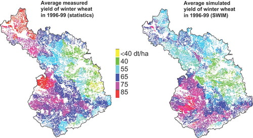
After validation for crop yield in a region, SWIM can be used for climate and land-use change impact assessment on agricultural production in addition to impacts on water resources. For example, the study of Huang et al. (2012) demonstrated an increased possibility to have two crop yields per year in the future in Germany under warmer climate conditions.

3.6.1 Lessons learnt

The main lesson learnt is that the vegetation and crop module is an important part of the ecohydrological model providing interfaces between water, vegetation and nutrients. However, its application for impact assessment requires additional testing for the reference period using observed or statistical data on crop yield. Crop rotations can be implemented and differentiated between soil classes based on the regional information.

3.7 Snow and glacier modules

In order to adequately simulate snow accumulation and snowmelt processes in alpine regions, the original degree-day snow module in SWIM was enhanced by using finer spatial units and including a more detailed description of snow processes. The hydrotopes, which serve as the basic spatial units of calculation, are further discretized by elevation bands. Besides snow melting, other processes, such as temporal change of the snow depth, refreezing of melting water and snow metamorphism, are included in the current snow module, adopting the method proposed by Gelfan et al. (2004). In addition, a simple glacier module was introduced to simulate glacier melt and glacier water accumulation. More detailed description of the snow and glacier modules is given in Huang et al. (2013b).

The extended snow module in SWIM enables a better calibration of the snow processes if observed snow data are available. In the Austrian and Swiss parts of the Danube and Rhine basins, long-term measured snow depth is available at 26 climate stations. In applications to the Upper Danube and the Upper Rhine basins, SWIM not only had to reproduce discharge in the rivers, but also snow cover in the alpine regions. This is especially important for climate impact assessment.

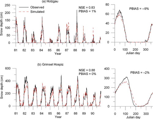
In general, snow depth could be well reproduced for 16 of the 26 stations with a NSE larger than 0.6 during the calibration period 1981–1990 at a daily time step. Figure 11 shows the comparison of simulated and observed snow depth (Fig. 11, left) at two selected climate stations. The simulated dynamics of snow accumulation show good agreement with the observed values for more than 60% of the stations. The corresponding average daily snow depths (Fig. 11, right) also confirm a good model performance for the validation period (1961–1980). At some stations, however, the snow depth was not reproduced adequately.

Fig. 11 Simulated and observed snow depth (left) at two selected climate stations for the period 1981–1990 and the corresponding average daily snow depth (right) for the same stations in the validation period (1961–1980).

Hence, in the future the extended snow model in SWIM has to be tested for some medium-scale catchments with finer spatial resolution, where the detailed information on climate and river discharge at the outlet is available.

3.7.1 Lessons learnt

Representation of snow dynamics and snow patterns is very important for climate impact studies in regions where snow influences the flow regime. The widely used degree-day method for snow is too simplified, but its improvement is possible.

There are several possible reasons that make it difficult for SWIM to simulate snow dynamics using the extended snow module. First, the degree-day factor is not fully distributed as only the elevation information was considered to modify the degree-day factor spatially. Other data (e.g. radiation and slope aspect) were not included due to insufficient climate data and the semi-distributed structure of SWIM. Second, the bias between the interpolated and actual climate conditions at specific points leads to inaccuracies. Interpolation of the climate data into the centroids of sub-basins and then correction for each hydrotope based on its elevation characteristics can generate errors. Third, the spatial resolution of this study (250 m) might be too coarse to precisely simulate the point processes. However, an alternative method of using a fully distributed model at a fine resolution would require large computational resources, being much more data-intensive and not compatible with other modules.

Regarding the dynamics of glaciers, it is an even more complex problem: the glacier melt can be included in a model using a linear storage concept, but the dynamic modelling of glaciers for a period of 50–100 years is a challenge for future research.

3.8 Reservoirs and inundation

Impact studies in managed river basins require adequate representation of both natural processes and those influenced by land and water management. One such case study is the Upper Niger Basin in West Africa (~350 000 km²) including the Inner Niger Delta (IND) at its outlet. The catchment is subject to strong seasonal and inter-annual variation in rainfall and river flow (Zwarts et al. 2006). Rainfall is very unequally distributed in the basin, where the headwater regions receive up to 2000 mm during the rainy season, compared to only 200–500 mm in the IND. The IND is a large floodplain, and the total inundated area ranged between 6150 and 22 360 km² during the 1990s (according to Mahé et al. 2011). The large range is a result of the high inter-annual variability of rainfall, particularly in the Niger headwaters.

The IND is crucial to the support of livelihoods of 1.5 million people (crop farmers, fishermen and herders). Beside the importance of flooding conditions, low flow conditions during the dry season influence ecosystem functions and integrity, and are mainly affected by upstream water management. Beside some smaller dams, one major dam, Sélingué, with a capacity of 2.16 km³, was built in 1982 in the Upper Niger (Mali), and another large dam, Fomi, will be built in Guinea. To summarize, the IND represents a complex system characterized by inundation processes which in turn depend on climate and upstream water management.

In order to account for an existing and a planned large dam in the Niger headwaters and to simulate the impacts of upstream water management and climate variability on inundation patterns in the IND, it was necessary to develop two new modules for the SWIM model: a reservoir module and an inundation module.

The reservoir module for SWIM was developed by Koch et al. (2013). It implements three management options: (a) variable daily minimum discharge to meet discharge targets, e.g. environmental flow downstream under consideration of maximum and minimum water levels in the reservoir; (b) daily release based on firm energy yields by a hydropower plant at the reservoir (the release to produce the required energy is calculated depending on the water level); and (c) daily release depending on water level (rising/falling release with increased/lowered water level, depending on the objective of reservoir management).

The inundation module was required to assess the consequences of climate change and variability, and upstream water management on varying inflow patterns into the IND, and to simulate discharge at the wetland outlet. This module (Liersch et al. 2012a) accounts for flooding and release processes and considers increased infiltration and evaporation from the additional water surface. During the flood season, the water volume exceeding river channel capacity is diverted to sub-basin inundation storages. The process of water release from these storages back to the channel follows a recession constant, while the water trapped in ponds remains in the wetland area.

Figure 12 shows observed and simulated water discharge of the River Niger at Koulikoro (~121 000 km²) in the dry season (March–May) for two periods: 1970–1979 with unmanaged flows and 1990–1999, i.e. after the Sélingué Dam was built. Additionally, the simulated discharge for the 1990s without considering reservoir management is shown to demonstrate the impact of reservoir management. The fluctuations of the observed time series are caused by daily operations of the reservoir, which are sometimes defined according to weather forecasts or other very specific management requirements (this information was not available for the modelling). The model simulates reservoir outflow according to monthly rules derived from observations and planned long-term management.

Fig. 12 Reservoir module performance during the dry period with and without reservoir management for the Niger basin, gauge Koulikoro (121 000 km²).

As Fig. 12 demonstrates, the simulated unmanaged discharge during the 1990s is higher than the unmanaged discharge during the 1970s. This is a consequence of climatic differences in these two periods. However, with the construction of the Sélingué hydropower dam, low flows increased by 70%—from 59 m³/s in the 1970s to 161 m³/s in the 1990s. Figure 12 shows that the reservoir module in SWIM is able to adequately represent the operation strategies of the existing dam, thus considerably improving the low flow simulations in the 1990s. The module can be used to evaluate potential impacts of the planned dam projects.

Figure 13 shows the observed and simulated discharges at the IND outlet (gauge Dire) averaged over the period 1982–2000. The grey dashed line represents the simulated discharge without considering wetland-specific processes related to flooding and release of water in the IND. Neglecting those processes in the model leads to unrealistic simulation of flow dynamics at the wetland outlet with strong overestimation (PBIAS = 194%). Discharge during the rainy season is highly overestimated as it does not account for the tremendous water losses of 40% between inflow into and outflow out of the wetland. The black dashed line shows the simulated discharge with the inundation module included in SWIM. The PBIAS achieved with the inundation module is 22% proving a satisfactory representation of these processes in the model. The wetland influence on discharge during the rainy season is captured by the inundation module fairly well.

Fig. 13 Water discharge simulation with and without inundation module, average year representing both the calibration and validation periods.

3.8.1 Lessons learnt

This study confirms the importance of introducing reservoirs and inundation processes in an ecohydrological model. Although it is not trivial and requires additional data, it extends the model applicability to basins where these processes substantially influence river discharge. There is still room for further improvements of the inundation module in terms of physical representation of natural processes as well as input data quality.

4 CASE STUDIES ON CLIMATE AND LAND-USE CHANGE IMPACT

4.1 Germany study: seasonality of river discharge and low flow

Considering the effects of climate warming, impacts on water resources are among the main concerns worldwide. Recently, the first Germany-wide climate impact assessment of water resources, including changes in return periods of floods and low flows, was performed using SWIM driven by regional climate models (Huang et al. 2010, 2013a, 2013b, Hattermann et al. 2011). All five large river basins covering 90% of the German territory (cf. Section 3.1) were included. The calibration and validation results for five main gauges were good, with NSE values from 0.79 to 0.90 and PBIAS values from −8% to +6%. The validation for most intermediate gauges was also satisfactory (Table 3). A special focus of the study was on propagation of uncertainty. Here some results on changes in seasonality of river discharge and low flow frequency are presented.

4.1.1 Changes in seasonality of river discharge

The projections of seasonal river discharge in Germany were simulated using climate scenario produced by the statistical downscaling tool STAR (Orlowsky et al. 2008). STAR is able to generate multiple climate projections by implementing a random process, so that an ensemble of 100 realizations of one scenario can be produced. Until 2060, STAR projects a significant decrease of the annual precipitation in eastern and southeastern Germany, and an increase in the northwestern and western Germany, while the annual temperature is expected to rise by 2–3°C.

Figure 14 shows a comparison of the simulated average seasonal river discharge in the scenario period 2031–2060 and in the reference period 1961–1990 at six selected gauges. In the scenario period, the changes in seasonal water discharge are different between the basins and seasons, and some of them are strong. Winter discharge is likely to increase practically in all rivers (except the Neckar), and especially in the Ems and Weser located in northwestern Germany (80–100% of the projections). The recession of the winter flow tends to start earlier in spring and last longer into late summer.

Fig. 14 Seasonal water discharge in the scenario periods (2031–2060) including 80 (dark grey) and 100 (light grey) realizations and the median of 100 realizations (black line) compared to the simulated discharge for the reference period 1961–1990 for six basins: (a) the Ems (gauge Versen); (b) the Weser (gauge Intschede); (c) the Saale (gauge Calbe-Grizehne); (d) the Danube (gauge Hofkirchen); (e) the Main (gauge Frankfurt-Osthafen); and (f) the Neckar basin (gauge Rockenau SKA).

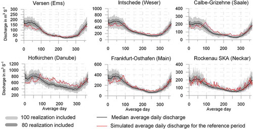
All the rivers are likely to have lower discharge from July to September due to higher evapotranspiration in a warmer climate, and lack of increased summer precipitation that could compensate for the enhanced evapotranspiration. The earlier harvest of winter crops and the following faster growth of cover crop aggravate the loss of soil water and decrease of runoff in corresponding months. Among the six river basins, the discharge decreases in summer and autumn most dramatically in the Danube, Saale and Neckar basins (by approx. 17–24%), where almost all 100 scenario realizations indicate a decrease. It is also worth mentioning that, in all rivers except the Danube, the water discharge is already very low in the current autumn period, and the projected mean river flow in the Saale in 2031–2060 approaches zero. However, the low-flow augmentation with the help of the reservoirs of the Saale cascade (Qmin = 5 m³/s) was not included in the simulation.

4.1.2 Changes in low-flow frequency

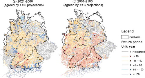
The potential impact of climate change on the frequency of extreme low flows in Germany was investigated using SWIM driven by climate scenarios from three regional climate models (RCMs): REMO (Tomassini and Jacob 2009), CCLM (Böhm et al. 2006) and WettReg (Enke et al. 2005a, 2005b). In total, the three models generated 10 climate scenarios including various emissions scenarios (A1B, A2 and B1). First, the level of the 50-year low flow was estimated for the reference period 1961–2000. After that, the occurrence of the current 50-year low flow (i.e. from the reference period) was calculated in the two scenario periods (2021–2060 and 2061–2100) for 5473 river reaches in Germany applying the GEV distribution (see more details in Huang et al. 2013b).

Figure 15 shows the medium return period for each river reach in two scenario periods, highlighting the river reaches where at least six of the 10 scenario results agree. As can be seen in Fig. 15(a), rather small changes in low-flow frequencies are projected in the period 2021–2060, because the return periods agreed by six or more scenarios vary mostly between 10 and 40 years. In the second period 2061–2100, however, much more frequent low flows are projected in southern and part of central Germany (Fig. 15(b), red colour indicates that the current 50-year low flow may occur in less than 10 years). There is larger uncertainty of the change patterns in the northern part of Germany, and a less dramatic increase in low flow frequency, except in the Saale and Mulde sub-basins of the Elbe. For the rivers in the Austrian alpine region less frequent low flows are projected compared to the reference period in both periods.

Fig. 15 Median return period for the 50-year low flow (averaged from those driven by REMO, CCLM and Wettreg scenarios) with the change directions agreed by 6–10 projections for the periods (a) 2021–2060 and (b) 2061–2100.

Lessons learnt are summarized in the next section.

4.2 Germany study: climate impact on floods and flood-caused damages

Floods are the most common and widespread of all recurrent natural disasters. Potential changes in flood hazard (intensity and probability of the event) and flood risk (combination of the hazard, exposure and vulnerability of the affected system, see Merz 2006) caused by changes in climate and land use are a major concern (Kundzewicz and Schellnhuber 2004).

An increase in flood-prone weather patterns with intense precipitation and high river flows is observed in Germany over the last 60 years (Hattermann et al. 2012, 2013). The possible rise in flood-caused damage to buildings and infrastructure under a changing climate is of particular interest to the insurance sector. In the following, some results of a modelling study commissioned by the Association of German Insurers (GDV) are presented. The aim of the study was to analyse the projected trends in flood generation and related damages (Hattermann et al. 2014).

The hydrological modelling and assessment of flood conditions under a changing climate was performed with SWIM (Huang et al. 2013a) for the same five major river basins in Germany as described in sections 3.1 and 4.1. In total, 3766 river reaches in the five basins were considered in the simulations. The climate scenarios used in the study were from two German RCMs, namely REMO and CCLM. Overall, three REMO scenarios (A1B, A2 and B1) and two CCLM scenarios (A1B and B1, each with two realizations) were applied.

The procedure of estimating the financial losses caused by riverine floods took advantage of the fact that the damage values are functions of the flood return period. These locally specific flood damage functions (different for each river section and taking into account density of buildings and enterprises) were provided by the GDV. The flood return periods estimated for two scenario periods (2021–2060 and 2061–2100) were then compared to the ones estimated for the control period based on simulations using the same climate models as drivers.

Figure 16 (left) illustrates the results for the reference period showing the return periods of simulated and observed flows above the threshold of the 95th percentile fitted to generalized Pareto distribution (GPD) curves at gauge Achleiten (Danube). The corresponding damages for this river section, calculated with observed and simulated runoff, applying the damage functions provided by the GDV, are depicted in Fig. 16 (right). One can see that the model is able to reproduce extreme flood events under reference conditions, and also the related flood damages are well comparable. It has to be mentioned that the results are not so good in highly regulated river systems where management dominates flood generation processes.

Fig. 16 Left: extreme value functions (GPD) fitting the observed and simulated daily flows at gauge Archleiten (Danube) in the period 1951–2000; right: comparison of flood damages at river section Archleiten in 1961–2000 calculated using runoff simulated by SWIM (sim) and observed runoff (obs) and applying damage functions provided by the German Insurance Association (GDV).

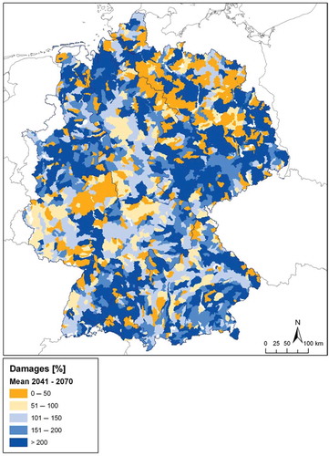
Figure 17 shows a map of projected changes in flood-related damages in Germany per river section as a summary of all seven scenario realizations. The estimation of damages followed the method described above. The trends are mostly positive, i.e. showing the projected increase in damage, in the mid-western and mid-eastern areas, windward parts of the mountains and the corresponding river sections, and in northwestern Germany. For a more detailed description of the method and results see Hattermann et al. (2014).

Fig. 17 Relative changes in flood related damages as average values of seven scenario runs in 2041–2070 compared to the average damages in 1961–2000 (defined as 100%). For further explanations see Hattermann et al. (2014).

It is worth mentioning that the methods applied here, i.e. using the return period of an event as link to the damages and not the absolute discharge level, enables the use of climate scenario data without bias correction for flood damage modelling, because it is not the absolute value that matters for the return periods but rather the probability of occurrence. However, the bias in climate data should be analysed first and should be reasonably low in order to have flood generating processes comparable to those under reference climate conditions.

4.2.1 Lessons learnt

The lessons learnt in climate impact studies described in sections 4.1 and 4.2 can be listed as follows:

1. if the assessment is done for large regions, multi-site calibration and validation are needed (as described above in sections 3.1 and 3.2);

2. if the climate impact study focuses on extreme events, the usual hydrological calibration and validation are not sufficient, and special testing on how well the model reproduces high and low flows is necessary;

3. the use of climate scenarios from dynamical RCMs or downscaled GCMs should be preferred, especially for the analysis of extremes, and ensembles of climate scenarios should be used if possible for better estimation of uncertainty;

4. simulations for the future should be compared with simulations for the reference period driven by the same climate model (not by observations);

5. the simulation of impacts of climate change is inevitably connected with uncertainties, partly due to the uncertainties of climate scenarios and input data, and partly due to the impact model structure and model parameterization;

6. the projections of extreme events are more uncertain than projections of mean conditions. Besides, our recent study (Huang et al. 2014) has shown that bias correction does not improve reliability, nor does it decrease uncertainty for flood projections.

4.3 Land-use change impact on water quantity and quality

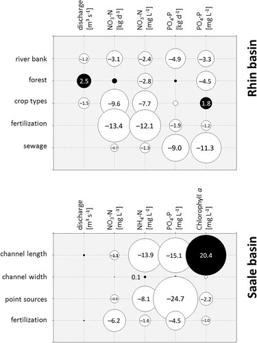
Changes in land and water management can significantly influence water quantity and quality in a river basin. Ecohydrological river basin models can be used as tools to support the implementation of measures for improving water quality in watersheds. Two examples of SWIM applications for the evaluation of land-use change scenarios are presented in Fig. 18 with corresponding explanations in Table 4. The aim of the studies was to find measures to reduce nutrient concentrations and to improve the ecological status in two tributaries within the Elbe catchment. On the one hand, direct measures dealing with reduction of the point and diffuse nutrient pollution were tested. On the other hand, possible indirect methods (e.g. restoration of wetlands), aimed at reaching a more natural status of the river ecosystem, were analysed.

Table 4 Description of the land-use and management change scenarios simulated with SWIM in two different sub-catchments of the Elbe basin in Germany (reference periods for the Rhin basin: 2001–2005, for the Saale basin: 1996–2003).

Scenario	Description
Rhin basin:
River bank	Conversion of fertilized agricultural land within 50 m around rivers and lakes to extensive grassland without fertilization
Forest	Conversion of all forested areas (34% of the whole catchment) to deciduous forests (reference: 80% evergreen)
Crop types	Change of crop types needing most fertilization (rape, beet and maize) to winter wheat
Fertilization	Maintaining the reference situation for crop types composition but reducing crop specific N and P fertilization by 20%
Sewage	Reducing the NO3-N emissions of all sewage treatment plants within the catchment by 10% and the PO4-P emissions by 20%
Saale basin:
Channel length	Extension of all channel lengthes per sub-basin by 20%
Channel width	Enlargement of all channel widths per sub-basin by 20%
Point sources	Reduction of all point source emissions (N by 10% and P by 20%)
Fertilization	Reduction of all fertilizer amounts by 20%

Fig. 18 Percentage change of selected mean SWIM model outputs under land-use change scenario conditions compared to the reference conditions in two different catchments within the Elbe River basin (for detailed description of the single scenario conditions see Table 4). The size of circle represents the increase (black) and decrease (white) in percent scaled to 100.

4.3.1 Scenarios for the Rhin

The first study was applied to the Rhin catchment, with a drainage area of 1716 km² (Hesse et al. 2008), and demonstrated how nutrient load reduction can be achieved (Fig. 18, upper graph). It was found that NO₃-N is more sensitive to changes in fertilization regime and crop type composition, whereas PO₄-P can be reduced most effectively by decreasing point source emissions. This can be explained by the relative influence of point and diffuse pollution on the total loads of nutrients in the region: nitrate N loads originate mostly from diffuse sources, and phosphate P is mainly introduced to the river system by point sources (sewage effluents). A change of crop types to species that demand less nutrients and more water even leads to an increase of PO₄-P concentrations and lower discharge in the river due to weaker dilution of point source-based PO₄-P with lower discharge. The highest decrease in PO₄-P concentration could be achieved by reducing the inflow of nutrients with sewage waters. An upgrading of the sewage treatment facilities has higher influence on potential PO₄-P reduction compared to that of NO₃-N.

The installation of buffer zones without agricultural use around surface water bodies led to decreased nutrient loads. In contrast, the conversion of all evergreen and mixed forests to deciduous ones marginally increased the nutrient loads of the river. However, the concentrations decreased due to higher discharge at the outlet of the basin (caused by reduced transpiration of deciduous trees in winter months) and dilution processes.

The land-use scenario results for the Rhin have shown that nutrient concentrations in the river are more sensitive to changes in fertilization regime and point source emissions than to changes in the composition of land-use patterns.

4.3.2 Scenarios for the Saale

The land-use change assessment for the larger Saale watershed (24 130 km²), also belonging to the Elbe River basin, revealed quite similar results regarding the influence of point and diffuse sources on the nutrient concentrations (Fig. 18, lower graph) (Hesse et al. 2012). Nutrients originating mainly from point sources (here: PO₄-P and NH₄-N) are more sensitive to changes in sewage and industrial effluents, whereas NO₃-N could be decreased most effectively by fertilizer reduction. In general, a reduction of point sources seems to have a more direct and straightforward influence on the river system. So, a 20% decrease of PO₄-P from point sources resulted in up to 20% reduction of PO₄-P concentration in the river, whereas a 20% reduction of fertilizers decreased nutrient concentrations by less than ten percent. Due to the reduced nutrient concentrations in the river water the chlorophyll a concentrations were slightly diminished, too.

The two other simulated management experiments dealing with enlargement of river width and length aimed at improving the river's morphology. An increase of channel length resulted in a decrease of nutrient concentrations but increased the phytoplankton biomass due to increased water retention time. The change in channel width, in contrast, had almost no influence on the observed concentrations of nutrients and phytoplankton. The results of the simulation experiments for the Saale basin show the relative importance of physical boundary conditions on phytoplankton. Therefore, measures to improve water quality should not only consider the nutrient input amounts and composition, but also the river morphology.

4.3.3 Lessons learnt

Our studies revealed a higher sensitivity of NO₃-N pollution to diffuse sources (fertilization in agriculture), and that of PO₄-P pollution to point source emissions (sewage treatment plants) in two catchments belonging to the Elbe basin. Besides, the importance of physical boundary conditions (climate, river morphology and land-use patterns) on concentrations and loads of nutrients in rivers was confirmed. However, the results are region-specific, as they depend on physiographic setting and anthropogenic influences.

Models like SWIM are useful for impact assessment, but there are still limits and restrictions: not all land-use changes that are of interest to stakeholders can be implemented in the model, and not all easily modelled scenarios can be realized. Land-use change can be considered for analysis of climate change impacts on water quality, and combined climate and land-use change scenarios may be helpful in land-use planning in order to increase the adaptive capacity of river basins.

4.4 Impact on water availability and floating rice in the Upper Niger basin

The last example in this section presents an impact assessment for the Upper Niger basin in the West African Sahel covering an area of about 350 000 km² and including the IND at its outlet. The study area and the reservoir and inundation modules in application to this case study were already described briefly in Section 3.8 above.

The SWIM model was applied for the Upper Niger basin in order to assess the impacts of climate change and water management on water resources and floating rice (Oryza glaberrima) production in the IND (see more details in Liersch et al. 2012a, 2012b). The objective of the study was to investigate the carrying capacity of the IND in terms of the number of people that can be supported by the ecosystem services related to floating rice production by 2050.

Impacts of climate change were investigated by using the statistical regional climate model STAR (Orlowsky et al. 2008) projecting future climate for the period 2011–2050 with WATCH forcing data (Weedon et al. 2011) from 1960–2001. The ‘observational’ time series was rearranged in order to develop three scenarios, each with 100 realizations. A 0°C scenario was used to assess climate impacts representing conditions at the end of the 20th century. The 0.75°C scenario is a continuation of the recent temperature trend, and the 1.5°C scenario represents further temperature increase. Whereas rainfall does not change significantly in the 0°C scenario, the other two scenarios are characterized by a rather strong decline of rainfall amounts.

The impacts of reservoir management on inflows into the IND and flooding processes were simulated under consideration of one major dam (Sélingué) with a capacity of 2.16 km³, and another large dam (Fomi in Guinea), which is in the planning phase (cf. 3.8).

The future carrying capacity of the IND to support floating rice production was assessed in the following way. The inundation module (see section 3.8) was used to simulate areas within the IND that are suitable for floating rice production, being inundated by 1–2 m for a duration of at least 90 days. The productivity of this rice species is 1–2 t/ha. Floating rice is the main staple crop in the IND and is used as a surrogate for cereal production. According to the national plan of Mali (RDM 2010), cereal consumption is about 214 kg/person per year. Based on these assumptions, the potential carrying capacity of the IND was calculated as the product of suitable area and the productivity. Divided by cereal consumption per capita, the number of people that could be potentially supported by the ecosystem service of cereal production was calculated. Scenario results are shown in Fig. 19 and Table 5.

Table 5 Wetland capacity for rice production to support people (units: number of people in million) in the IND for the period 2041–2050.

Scenario	No dams mean	Both dams mean	Total diff.	Rel. diff. (%)
0.0°C	1.5	1.45	−0.05	−3.3
0.75°C	0.93	0.81	−0.12	−13
1.5°C	0.53	0.43	−0.1	−19

Fig. 19 Simulated carrying capacity of rice production in the Inner Niger Delta. Continuous coloured lines represent the means of 100 realizations for the three scenarios without upstream reservoirs. Dashed lines represent the means of 100 realizations with two upstream reservoirs included in simulations. The coloured bands represent 33–66 percentiles of 100 realizations.

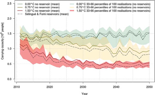
The carrying capacity of the IND to support floating rice production and therefore the nutrition of the population ranges between 1.0 and 1.8 (mean = 1.5) million people that can be fed in the period 2041–2050 under the 0.0°C scenario, considering the 33th and 66th percentiles of 100 realizations and assuming no reservoirs upstream. The combined impact of both dams leads to a reduction in carrying capacity by 3.7% or 55 000 people due to evaporation losses from open water surface of the reservoirs.

The range in the 0.75°C scenario is between 0.5 and 1.4 (mean = 0.93) million people. The difference in the average carrying capacity between 0.0°C and 0.75°C scenario is 0.57 million people. The combined impact of both dams in the 0.75°C scenario leads to a further reduction in carrying capacity by 13% or 120 600 people.

The range in the 1.5°C scenario is between 0.34 and 0.63 (mean = 0.53) million people. The difference in the average carrying capacity between 0.0°C and 1.5°C scenario is about one million people. The combined impact of both dams in the 1.5°C scenario leads to a further reduction in carrying capacity by 19% or 101 700 people.

Climate change as projected by the STAR approach has very significant and serious consequences for the production of floating rice in the IND. The impact of additional reservoirs in the upstream basin would deteriorate the situation by decreasing the carrying capacity of the IND for floating rice production. Climate projections provided by other regional climate models are currently applied to the Upper Niger basin in order to better account for uncertainties related to regional climate modelling.

4.4.1 Lessons learnt

Assessing the impacts of changing boundary conditions requires adequate tools, namely reliable scenario data and appropriate models. The question of appropriateness of tools depends on the characteristics of the impact, the system under study and the issues to be investigated. Whereas conceptual models might be sufficient to study the impacts of climate change on the general water balance in basins with negligible management, more sophisticated approaches are required in the context of basins with inundation and reservoirs, such as in the Niger basin. The SWIM model with reservoirs and inundation modules can be used also for current water management scenarios and can be transferred to other basins with similar features.

5 SUMMARY AND OUTLOOK

Good calibration and validation results of hydrological models in gauged catchments with a dense network of good-quality climate and precipitation stations and minor water management are often demonstrated. It is much more difficult to obtain reasonable simulation results in poorly gauged basins and in basins with intensive water management. The SWIM model has proven itself versatile and applicable in a range of situations, from well gauged areas (e.g. in Germany), to developing countries, where the data are poor or are not easily available (e.g. in international river basins, where the neighbour countries do not wish to share the data).

One of the principal applications of the SWIM was in the major project GLOWA-Elbe, sponsored by the German Federal Ministry of Education and Research, embracing the Elbe basin (Wechsung et al. 2008). In the GLOWA-Elbe project, the SWIM-based toolbox was interactively coupled with a water management model. This development brought a refined groundwater representation with an altered evapotranspiration method, rendering the model capable of handling anthropogenic groundwater abstraction and recharge. The application of SWIM in the GLOWA-Elbe project allowed extensive testing of the model and stimulated its further development. For the whole Elbe River basin (approx. 45 000 hydrotopes), the model run time was 2.5 h for a simulation of 10 years. Stochastic investigations were accelerated by parallel computing.

SWIM was originally developed for use mainly in Europe and the temperate zone, and then successfully applied in other regions. So far, SWIM has been applied for assessments of water resources and climate impacts in four continents: Europe (with multiple applications in Germany, and some in the Czech Republic, Poland, Russia, Ukraine, Spain and Portugal), Asia (Yellow, Jinghe, Tailan, Aksu in China and Ganges in India and Bangladesh), large international rivers in Africa (Blue Nile, Niger, Oubangui and Limpopo), and South America (Sao Francisco in Brazil).

The intercomparison of impacts using several models is necessary in order to overcome the fragmentariness of projections produced by many models for different regions using different scenarios and methodologies, which are hardly comparable. Though these studies are of value in their own right, a quantitative synthesis of climate impacts, including consistent estimates of uncertainties, is missing. To ensure that climate change impact research meets the demands of decision makers at the regional scale for reliable information, projections of climate impacts must be provided at the regional scale, and compared between different models. Bridging the scales between global and regional impact research and models is also needed, and can go in both directions. SWIM is now being used as one of the tools for the intercomparison of impacts.

Application of SWIM for climate impact assessments is now extended by (a) including new regions overseas (e.g. Aich et al. 2014); (b) intercomparison of impacts simulated by several hydrological models and an ensemble of climate scenarios (e.g. Vetter et al. 2015); and (c) intercomparison of impacts simulated by SWIM and global models: the Land Dynamic Global Vegetation and Water Balance Model (LPJmL, Bondeau et al. 2007) and WaterGAP (Alcamo et al. 2003) for the regions in Europe and Africa.

SWIM has been successfully tested to represent various hydrological conditions. However, one should be cautious about potential problems and restrictions in the use of SWIM for some processes or areas, such as operational flood forecasting, forest dynamics (except for a special model version which requires regional forest inventory data), long-term glacier dynamics, intensively managed catchments if management data is not available, small catchments (< 100 km²), karst-influenced watersheds, river basins with permafrost, which are beyond the areas of recommended applications of the model. Besides, difficult challenges come about when modelling: (a) mountainous catchments with glaciers, when observed climate data are only from the lowland part, and have to be extrapolated to the whole area, and (b) catchments where the runoff coefficient is low (2–3%), and average annual water use is approaching water availability. The use of SWIM in data-scarce regions requires previous modelling experience, and an additional analysis of data. The model can be used in ungauged basins only after its calibration in a gauged catchment with similar conditions belonging to the same region, and after quantification of parameter uncertainty (Hattermann et al. 2005).

In our view, lessons learnt summarized at the end of sub-sections above are mostly valid also for other process-based hydrological models of intermediate complexity. Application of simpler precipitation-runoff models not accounting for water-vegetation interactions and some specific features (reservoirs, glaciers, etc.) for impact assessment could be problematic in some regions.

Newly developed and enhanced modules allow fixing some of the problems listed above. Further test and development is ongoing for the following processes: snow and glacier dynamics, irrigation using different water sources and methods, vegetation growth in tropical regions, and reservoir management. However, new modules make the model computationally more demanding and their use still requires additional testing (all comes at a cost). As the model is complex (not a ‘push-button’ model), it should be used only by experienced or specially trained modellers.

Drainage basins in many parts of the world are either ungauged or inadequately gauged and the situation is worsening because the existing observation networks are in decline. At the same time, water resources are under a growing threat in a world that is becoming more populated and where the demand for water per capita is constantly increasing. Therefore, while the supply of data declines, the need for such data increases (WMO 2009). This poses a considerable challenge to the hydrological and water resources communities, to assess and manage freshwater resources with an inadequate supply of data. The SWIM lends itself well as an useful, and well tested model also in data scarce situations.

The modest data requirements are an important advantage of the model. Direct connection to land-use and climate data provides a possibility to use the model for analysis of climate change and land-use change impacts on hydrology, agricultural production, and water quality. Hence, the model represents an example of a useful tool to facilitate river basin management and to bridge the gap between science and policy. The lessons learnt from the multiple applications of SWIM could be useful for a broad community of regional impact modellers.

Disclosure statement

No potential conflict of interest was reported by the author(s).

REFERENCES

- Abbott, M.B., et al., 1986. An introduction to the european hydrological systems-systeme hydrologique Europeen, ‘SHE’. 2. Structure of a physically based distributed modelling system. Journal of Hydrology, 87, 61–77. doi:10.1016/0022-1694(86)90115-0
- Aich, V., et al., 2014. Comparing impacts of climate change on streamflow in four large African river basins, Hydrology and Earth System Sciences, 18, 1305–1321. doi:10.5194/hess-18-1305-2014
- Alcamo, J., et al., 2003. Development and testing of the waterGAP 2 global model of water use and availability. Hydrological Sciences Journal, 48 (3), 317–337. doi:10.1623/hysj.48.3.317.45290
- Arnold, J.G., Allen, P.M., and Bernhardt, G., 1993. A comprehensive surface-groundwater flow model. Journal of Hydrology, 142 (1–4), 47–69. doi:10.1016/0022-1694(93)90004-S
- Arnold, J.G., et al., 1990. SWRRB - A basin scale simulation model for soil and water resources management. College Station, TX: Texas A&M University Press.
- Bergström, S., 1995. The HBV model. In: V.P. Singh, Ed. Computer models of watershed hydrology. Highlands Ranch, CO: Water Resources Publications, 443–476.
- Beven, K.J. and Kirby, M.J., 1979. A physically based variable contributing area model of basin hydrology. Hydrological Sciences Bulletin, 24 (1), 43–69.
- Böhm, U., et al., 2006. CLM – The climate version of LM: brief description and long-term application. Proceedings from the COSMO General Meeting 2005. COSMO Newsletter [online], 6, 225–235. Available from: http://www.cosmo-model.org [Accessed 6 Feb 2014].
- Bondeau, A., et al., 2007. Modelling the role of agriculture for the 20th century global terrestrial carbon balance. Global Change Biology, 13 (3), 679–706. doi:10.1111/j.1365-2486.2006.01305.x
- Boyacioglu, H., et al., 2011. Modeling the impacts of climate change on nitrogen retention in a 4th order stream. Climatic Change. doi:10.1007/s10584-011-0369-1
- Brown, L.C. and Barnwell, T.O., 1987. The enhanced water quality models QUAL2E and QUAL2E-UNCAS: documentation and user manual. Athens, GA: USEPA, EPA/600/3-87/007.
- Chiew, F.H.S. and McMahon, T.A., 1993. Assessing the adequacy of catchment streamflow yield estimates. Australian Journal of Soil Research, 31, 665–680. doi:10.1071/SR9930665
- Coles, S., 2001. An introduction to statistical modeling of extreme values. Heidelberg: Springer.
- Conradt, T., et al., 2012. Spatially differentiated management-revised discharge scenarios for an integrated analysis of multi-realisation climate and land use scenarios for the Elbe River basin. Regional Environmental Change. doi:10.1007/s10113-012-0279-4
- Enke, W., et al., 2005a. Results of five regional climate studies applying a weather pattern based downscaling method to ECHAM4 climate simulations. Meteorologische Zeitschrift, 14 (2), 247–257. doi:10.1127/0941-2948/2005/0028
- Enke, W., Schneider, F., and Deutschländer, T., 2005b. A novel scheme to derive optimized circulation pattern classifications for downscaling and forecast purposes. Theoretical Applications Climatology, 82, 51–63. doi:10.1007/s00704-004-0116-x
- Gassman, P.W., et al., 2010. Invited Review Article: The agricultural policy/environmental eXtender (APEX) model: an emerging tool for landscape and watershed environmental analyses. Transactions of the ASABE, 53 (3), 711–740. doi:10.13031/2013.30078
- Gelfan, A.N., Pomeroy, J.W., and Kuchment, L.S., 2004. Modeling forest cover influences on snow accumulation, sublimation, and melt. Journal of Hydrometeorology, 5 (5), 785–803. doi:10.1175/1525-7541(2004)005<0785:MFCIOS>2.0.CO;2
- Grünewald, U., 2001. Water resources management in river catchments influenced by lignite mining. Ecological Engineering, 17, 143–152. doi:10.1016/S0925-8574(00)00154-3
- Harley, P.C., et al., 1992. Modelling photosynthesis of cotton grown in elevated CO2. Plant, Cell and Environment, 15 (3), 271–282. doi:10.1111/j.1365-3040.1992.tb00974.x
- Hattermann, F.F., Krysanova, V., and Hesse, C., 2008. Modelling wetland processes in regional applications. Hydrological Sciences Journal, 53 (5), 1001–1012. doi:10.1623/hysj.53.5.1001
- Hattermann, F.F., et al., 2004. Integrating groundwater dynamics in regional hydrological modelling. Environmental Modelling & Software, 19 (11), 1039–1051. doi:10.1016/j.envsoft.2003.11.007
- Hattermann, F.F., et al., 2005. Runoff simulations on the macroscale with the ecohydrological model SWIM in the Elbe catchment - validation and uncertainty analysis. Hydrological Processes, 19 (3), 693–714. doi:10.1002/hyp.5625
- Hattermann, F.F., et al., 2006. Integrating wetlands and riparian zones in river basin modelling. Ecological Modelling, 199 (4), 379–392. doi:10.1016/j.ecolmodel.2005.06.012
- Hattermann, F.F., et al., 2011. Model-supported impact assessment for the water sector in Central Germany under climate change—A case study. Water Resources Management, 25 (13), 3113–3134. doi:10.1007/s11269-011-9848-4
- Hattermann, F.F., et al., 2012. Flood risk in holistic perspective—observed changes in Germany. In: Z.W. Kundzewicz, ed. Changes in flood risk in Europe. Wallingford: International Association of Hydrological Sciences IAHS Special publ. 10, 212–237.
- Hattermann, F.F., et al., 2013. Climatological drivers of changes in flood hazard in Germany. Acta Geophysica, 61 (2), 463–477. doi:10.2478/s11600-012-0070-4
- Hattermann, F.F., et al., 2014. Modeling flood damages under climate change conditions - a case study for Germany. Natural Hazards and Earth System Science, 14, 3151–3168. doi:10.5194/nhess-14-3151-2014
- Hesse, C., et al., 2008. Eco-hydrological modelling in a highly regulated lowland catchment to find measures for improving water quality. Ecological Modelling, 218 (1–2), 135–148. doi:10.1016/j.ecolmodel.2008.06.035
- Hesse, C., et al., 2013. Comparison of several approaches representing terrestrial and in-stream nutrient retention and decomposition in watershed modelling. Ecological Modelling, 269, 70–85. doi:10.1016/j.ecolmodel.2013.08.017
- Hesse, C., Krysanova, V., and Voß, A., 2012. Implementing in-stream nutrient processes in large-scale landscape modeling for the impact assessment on water quality. Environmental Modeling & Assessment, 17 (6), 589–611. doi:10.1007/s10666-012-9320-8
- Holsten, A., et al., 2009. Impact of climate change on soil moisture dynamics in Brandenburg with a focus on nature conservation areas. Ecological Modelling, 220 (17), 2076–2087. doi:10.1016/j.ecolmodel.2009.04.038
- Huang, S., 2012. Modelling of environmental change impacts on water resources and hydrological extremes in Germany. Thesis (PhD). Potsdam University, Potsdam.
- Huang, S., Krysanova, V., and Hattermann, F.F., 2012. Impacts of climate change on water availability and crop yield in Germany. In: R. Seppelt, et al., eds. Proceedings of the International Congress on Environmental Modelling and Software: Managing Resources of a Limited Planet, Sixth Biennial Meeting, 2012 Leipzig.
- Huang, S., Krysanova, V., and Hattermann, F.F., 2013. Projection of low flow conditions in Germany under climate change by combining three RCMs and a regional hydrological model. Acta Geophysica, 61 (1), 151–193. doi:10.2478/s11600-012-0065-1
- Huang, S., Krysanova, V., and Hattermann, F., 2014. Does bias correction increase reliability of flood projections under climate change? – A case study of large rivers in Germany. International Journal of Climatology, 34 (14), 3780–3800. doi:10.1002/joc.3945
- Huang, S., et al., 2009. From meso- to macro-scale dynamic water quality modelling for the assessment of land use change scenarios. Ecological Modelling, 220 (19), 2543–2558. doi:10.1016/j.ecolmodel.2009.06.043
- Huang, S., et al., 2010. Simulation of spatiotemporal dynamics of water fluxes in Germany under climate change. Hydrological Processes, 24 (23), 3289–3306. doi:10.1002/hyp.7753
- Huang, S., et al., 2015. Impact of intensive irrigation activities on river discharge under agricultural scenarios in the semi-arid Aksu river basin, northwest China. Water Resources Management, 29 (3), 945–959. doi:10.1007/s11269-014-0853-2
- Huang, S., et al., 2013a. Projections of climate change impacts on river flood conditions in Germany by combining three different RCMs with a regional eco-hydrological model. Climatic Change, 116 (3–4), 631–663. doi:10.1007/s10584-012-0586-2
- Kimball, B.A., et al., 1995. Productivity and water use of wheat under free-air CO2 enrichment. Global Change Biology, 1, 429–442. doi:10.1111/j.1365-2486.1995.tb00041.x
- Knisel, W.G., ed., 1980. CREAMS: A field scale model for chemicals, runoff, and erosion from agricultural management systems. USDA Conservation Research Report, 26. Washington, DC: USDA.
- Koch, H., Liersch, S., and Hattermann, F.F., 2013. Integrating water resources management in eco-hydrological modelling. Water Science and Technology, 67 (7), 1525–1533. doi:10.2166/wst.2013.022
- Krysanova, V. and Arnold, J.G., 2008. Advances in ecohydrological modelling with SWAT—a review. Hydrological Sciences Journal, 53 (5), 939–947. doi:10.1623/hysj.53.5.939
- Krysanova, V. and Becker, A., 1999. Integrated modelling of hydrological processes and nutrient dynamics at the river basins scale. Hydrobiologia, 410, 131–138. doi:10.1023/A:1003728419934
- Krysanova, V. and Haberlandt, U., 2002b. Assessment of nitrogen leaching from arable land in large river basins. Part I: simulation experiments using a process-based model. Ecological Modelling, 150 (3), 255–275. doi:10.1016/S0304-3800(01)00525-7
- Krysanova, V., Hattermann, F., and Wechsung, F., 2007. Implications of complexity and uncertainty for integrated modelling and impact assessment in river basins. Environmental Modelling and Software, 22 (5), 701–709. doi:10.1016/j.envsoft.2005.12.029
- Krysanova, V., Müller-Wohlfeil, D.-I., and Becker, A., 1998. Development and test of a spatially distributed hydrological/water quality model for mesoscale watersheds. Ecological Modelling, 106 (2–3), 261–289. doi:10.1016/S0304-3800(97)00204-4
- Krysanova, V., Wechsung, F., and Hattermann, F., 2005. Development of the ecohydrological model SWIM for regional impact studies and vulnerability assessment. Hydrological Processes, 19, 763–783. doi:10.1002/hyp.5619
- Krysanova, V., et al., 1989. Simulation modelling of the coastal waters pollution from agricultural watershed. Ecological Modelling, 49 (1–2), 7–29. doi:10.1016/0304-3800(89)90041-0
- Krysanova, V., et al., 1999. Mesoscale ecohydrological modelling to analyse regional effects of climate change. Environmental Modeling and Assessment, 4 (4), 259–271. doi:10.1023/A:1019020518977
- Krysanova, V., et al., 2000. SWIM (Soil and Water Integrated Model): user manual. PIK Report no. 69. Potsdam: Potsdam Institute for Climate Impact Research.
- Krysanova, V., et al., 2002. Linkage between hydrological processes and sediment transport at the river basin scale - a modelling study. In: W. Summer and D.E. Walling, eds. Modelling erosion, sediment transport and sediment yield. Paris: UNESCO: International Hydrological Programme, IHP-VI, Technical Documents in Hydrology no. 60, 147–174.
- Kundzewicz, Z.W. and Schellnhuber, H.-J., 2004. Floods in the IPCC TAR perspective. Natural Hazards, 31 (1), 111–128. doi:10.1023/B:NHAZ.0000020257.09228.7b
- Liersch, S., et al., 2012a. Vulnerability of rice production in the Inner Niger Delta to water resources management under climate variability and change. Environmental Science and Policy. doi:10.1016/j.envsci.2012.10.014
- Liersch, S., et al., 2012b. Constraints of future freshwater resources in the Upper Niger Basin – Has the human-environmental system of the Inner Niger Delta a chance to survive? In: R. Seppelt, A.A. Voinov, and D. Bankamp, eds. Proceedings of the international congress on environmental modelling and software: Managing resources of a limited planet, Leipzig, Germany [online]. Available from: http://www.iemss.org/society/index.php/iemss-2012-proceedings [Accessed 21 November 2012].
- Mahé, G., et al., 2011. Estimation of the flooded area of the Inner Delta of the River Niger in Mali by hydrological balance and satellite data. In: S.W. Franks et al., eds. Hydro-climatology: variability and change, (Proceedings of symposium JHS02, Melbourne, Australia, July 2011). Wallingford: International Association of Hydrological Sciences, IAHS Publ. 344, 138–143.
- Mander, Ü., et al., 1997. Efficiency and dimensioning of riparian buffer zones in agricultural catchments. Ecological Engineering, 8 (4), 299–324. doi:10.1016/S0925-8574(97)00025-6
- Merz, B., 2006. Hochwasserrisiken: grenzen und Möglichkeiten der Risikoabschätzung. Stuttgart: Schweizerbart.
- Monteith, J.L., 1965. Evaporation and the environment. Symp. of the Society for Experimental Biology, 19, 205–234.
- Moriasi, D.N., et al., 2007. Model evaluation guidelines for systematic quantification of accuracy in watershed simulations. American Society of Agricultural and Biological Engineers, 50 (3), 885–900.
- Nash, J.E. and Sutcliffe, J.V., 1970. River flow forecasting through conceptual models part I—a discussion of principles. Journal of Hydrology, 10 (3), 282–290.
- Neteler, M. and Mitasova, H., 2008. Open source GIS: A GRASS GIS approach. 3rd ed. New York: Springer (ISBN-10: 038735767X; ISBN-13: 978-0387357676).
- Orlowsky, B., Gerstengarbe, F.-W., and Werner, P., 2008. A resampling scheme for regional climate simulations and its performance compared to a dynamical RCM. Theoretical and Applied Climatology, 92 (3–4), 209–223. doi:10.1007/s00704-007-0352-y
- Post, J., et al., 2008b. Integrated assessment of cropland soil carbon sensitivity to recent and future climate in the Elbe River basin. Hydrological Sciences Journal, 53 (5), 1043–1058. doi:10.1623/hysj.53.5.1043
- Post, J., et al., 2007. Evaluation of water and nutrient dynamics in soil-crop systems using the eco-hydrological catchment model SWIM. In: K.C. Kersebaum, et al., eds. Modelling water and nutrient dynamics in soil-crop systems. Dordrecht: Springer, 129–146.
- Post, J., et al., 2008a. Parameter and input data uncertainty estimation for the assessment of long-term soil organic carbon dynamics. Environmental Modelling and Software, 23, 125–138. doi:10.1016/j.envsoft.2007.05.010
- Priestley, C.H.B. and Taylor, R.J., 1972. On the assessment of surface heat flux and evaporation using large scale parameters. Monthly Weather Review, 100, 81–92. doi:10.1175/1520-0493(1972)100<0081:OTAOSH>2.3.CO;2
- RDM, 2010. Plan national d’investissement prioritaire dans le secteur agricole au Mali—2011–2015. Rapport PNIP-SA Republique du Mali, Bamako.
- Tomassini, L. and Jacob, D., 2009. Spatial analysis of trends in extreme precipitation events in high-resolution climate model results and observations for Germany. Journal of Geophysical Research, 114, D12113. doi:10.1029/2008JD010652
- Vetter, T., et al., 2015. Multi-model climate impact assessment and intercomparison for three large-scale river basins on three continents. Earth System Dynamics, 6, 17–43. doi:10.5194/esd-6-17-2015
- Wattenbach, M., et al., 2005. A simplified approach to implement forest eco-hydrological properties in regional hydrological modelling. Ecological Modelling, 187 (1), 40–59. doi:10.1016/j.ecolmodel.2005.01.026
- Wechsung, F., et al., eds., 2008. Integrated analysis of the impacts of global change on environment and society in the Elbe River Basin. Berlin: Weißensee Verlag.
- Wechsung, F., et al., 2000. May land use change reduce the water deficiency problem caused by reduced brown coal mining in the state of Brandenburg? Landscape and Urban Planning, 51 (2–4), 177–189. doi:10.1016/S0169-2046(00)00108-0
- Weedon, G.P., et al., 2011. Creation of the WATCH forcing data and its use to assess global and regional reference crop evaporation over land during the twentieth century. Journal of Hydrometeorology, 12, 823–848. doi:10.1175/2011JHM1369.1
- Williams, J.R. and Berndt, H.D., 1977. Sediment yield prediction based on watershed hydrology. Transactions of the American Society of Agricultural Engineers, 20 (6), 1100–1104. doi:10.13031/2013.35710
- Williams, J.R., et al., 1995. Simulation of animal waste management with APEX. In: J. McFarland, ed, Innovations and new horizons in livestock and poultry manure management. Austin, TX: Texas A&M University, Texas Agricultural Extension Service, 22–26.
- Williams, J.R., Renard, K.G., and Dyke, P.T., 1984. EPIC—a new model for assessing erosion’s effect on soil productivity. Journal of Soil and Water Conservation, 38 (5), 381–383.
- World Meteorological Organization (WMO), 2009. Modelling of hydrological systems. In: Guide to hydrological practices, vol. II—Management of water resources and application of hydrological practices, WMO-No. 168, 6th ed. Geneva: WMO, II.6-1–II.6.53.
- Wortmann, M., et al., 2013. Assessing the influence of the Merzbacher Lake outburst floods on discharge using the hydrological model SWIM in the Aksu headwaters, Kyrgyzstan/NW China. Hydrological Processes. doi:10.1002/hyp.10118
- Zwarts, L., et al., 2006. The economic and ecological effects of water management choices in the Upper Niger River: development of decision support methods. International Journal of Water Resources Development, 22, 135–156. doi:10.1080/07900620500405874