Hydrological response due to projected climate variability in Haw River watershed, North Carolina, USA

ABSTRACT

Global climate variations are expected to cause serious challenges to water resources planning and management, including an increase in sea level, abrupt changes in rainfall patterns and changes in ecosystems. This study evaluates impacts of mid-century climate variability as projected by climate models in the Haw River watershed, which contributes significantly to Jordan Lake, a major source of drinking water supply in central North Carolina, USA. The watershed-based hydrological model, Soil and Water Assessment Tool (SWAT), was successfully calibrated with very good to excellent performance. Projected precipitation and temperature information for 2040–2069 from four dynamically downscaled regional climate models (RCMs) was used to force the SWAT modeling set-up of the watershed. On a long-term basis, a 38% decrease in the precipitation in early fall is expected while spring months are expected to receive 30% higher precipitation compared to the baseline condition (1980–2009). Water yield was found to increase in spring months, with a maximum of 74% increase on average. Summer months are expected to have on average 8% higher evapotranspiration (ET) than the baseline. Analysis of the change in average monthly streamflow at the watershed outlet (which leads to Lake Jordan) shows that there might be, on average, an 80% increase in streamflow in spring months (February, March, April and May), with the greatest increase (107%) in May. In general, simulation results indicated that the hydrological response of the watershed is very sensitive to the potential variation in climate (precipitation and temperature), with precipitation being one of the decisive factors in water yield increase.

Editor Z.W. Kundzewicz Associate editor N. Verhoest

KEYWORDS:

• watershed modeling
• climate change
• SWAT
• RCM
• NARCCAP

1 Introduction

Water resources planning and management in the 21st century is becoming increasingly difficult due to conflicting demands from various stakeholder groups, ever increasing population, rapid urbanization and climate change affecting the hydrological cycles and regimes. Climate change has contributed to the uncertainty about water availability in the future. Based on the global climate models’ (GCMs) projections of the future climate, as reported by the Intergovernmental Panel on Climate Change (IPCC), temperatures in the 21st century are expected to be between 1.1 and 6.4°C higher than temperatures in the 20th century. The range of emissions scenarios studied suggest that greenhouse gas concentrations are expected to increase to between approximately 550 ppmv (parts per million by volume) in the 2030s and 660 ppmv by the 2050s (IPCC 2009). This projection is accompanied by changes in the amount and intensity of rainfall events. Precipitation on an average annual basis is expected to increase globally through to the end of the century, although the changes in the amount and intensity of precipitation will vary by region (IPCC 2007). For the USA, it is projected that heavy precipitation events would be more frequent. Heavy downpours that currently occur about once every 20 years are projected to occur about every four to 15 years by 2100, depending on location (USGCRP 2009).

In a recent IPCC special report on extreme events (IPCC 2012), it was emphasized that climate change has led to changes in climate extremes, and the social as well as physical dimensions of weather- and climate-related disasters were highlighted. Based on the projected global climate change impacts in the USA, several significant threats are projected for North Carolina. Being a coastal state, North Carolina’s extensive coastlines are under severe threat from global warming, which is expected to result in rising sea level to rise. Observations show that the sea level on North Carolina’s coast has risen approximately 0.30 m since observations began in the 1930s, and this is closely linked to broader global warming. North Carolina has been severely affected by drought twice in the recent past: in 2002 and again in 2007 (State Climate office of North Carolina; http://www.nc-climate.ncsu.edu/climate/climate_change).

Climate projections using GCM and regional climate models (RCMs) have been increasingly relied upon for impact assessment studies regarding hydrological cycle and watershed responses. Hydrological models are often coupled with climate scenarios generated from climate models to study climate change effects on water resources. Numerous studies in the past have focused on investigation of the hydrological behavior and response of different watersheds to anticipated climate change across the world at various spatial scales (Gleick and Chalecki 1999, Jha et al. 2004, 2006, Takle et al. 2005, 2010, Abdo et al. 2009, Abbaspour et al. 2009, Jha and Gassman 2013a, Jha et al. 2013b). Various approaches to impact assessment have been investigated in recent years, including regression-based GCM simulations (Stewart et al. 2004), dynamic downscaling of GCMs through nested climate models (Diffenbaugh et al. 2005), and climate model forcing of hydrological models (Christensen et al. 2004). In a recent study, Ficklin et al. (2013) used the combination of a hydrological model with 16 GCMs in the Upper Colorado River basin and found a temporal shift in most of the hydrological components, with significant snowmelt decline by the end of the 21st century under the A2 emissions scenario. Jha and Gassman (2013a), using the delta change method and ensembles of GCMs, found a 17% decrease in annual streamflow by mid-century in the Raccoon River watershed in the Midwest, with negative implications for the drinking water supply for central Iowa communities. In a similar investigation in the Boise and Spokane river watersheds, Jin and Sridhar (2012) found that the changes in precipitation (3.8 to 36%, and −6.7 to 17.9%, respectively) and temperature (0.02 to 3.9°C, and 0.1 to 3.5°C, respectively) by mid-century can cause peak streamflow to vary from −58 to +106 m³/s in the Boise River watershed and from −198 to +88 m³/s in the Spokane River watershed. The broad range of the hydrological predictions was attributed to the choice of climate models.

The objective of this study was to investigate the sensitivity of a watershed in the southeast USA for its hydrological response to potential changes in climate variability. The effort builds on an integrated approach of watershed modeling with various climate change scenarios. The Haw River watershed, draining an area of approximately 4000 km² in the north-central part of North Carolina, was evaluated for climate change impact assessment. The SWAT (Soil and Water Assessment Tool) model was used in the simulation of watershed hydrological processes. After successful calibration and validation with statistical validity, the modeling set-up was simulated using projected future climatic information from four RCMs. These scenarios are in compliance with the IPCC A2 SRES storyline (IPCC 2007) for the period 2040–2069, while the baseline corresponds to the period 1980–2009.

2 Material and methods

2.1 SWAT model description

The SWAT model is a long-term, continuous, watershed-scale simulation model that operates on a daily time step and is designed to assess the impact of different management practices on water, sediment and agricultural chemical yields. The model is distributed, computationally efficient, and capable of simulating at detailed spatiotemporal scales (Arnold et al. 1998). It simulates the hydrological cycle based on the water balance equation:

(1)

in which SW_t is the final soil water content (mm), SW₀ is the initial soil water content on day i (mm), t is the time (days), R_day is the amount of precipitation on day i (mm), Q_surf is the amount of surface runoff on day i (mm), E_a is the amount of evapotranspiration on day i (mm), W_seep is the amount of water entering the vadose zone from the soil profile on day i (mm), and Q_gw is the amount of return flow on day i (mm). Watersheds can be further subdivided into subwatersheds and further into hydrologic response units (HRUs) in SWAT to account for differences in soils, land use, crops, topography, weather, etc. After the simulations are performed at the HRU level they are aggregated and summarized at the subwatershed level. Total streamflow is estimated by summing up the runoffs from each of the subwatersheds. The water balance of each HRU is represented by four storage volumes: snow, soil profile, shallow aquifer and deep aquifer. SWAT incorporates a command structure to route runoff and chemicals through the watershed. Relevant details about how these processes are simulated can be found in the SWAT user’s manual (Neitsch et al. 2005). In this study, the modified Curve Number method to calculate partitioning of surface runoff vs infiltration, the Muskingum method for simulating the channel routing process, and the Hargreaves method for estimating potential evapotranspiration, were used as input options.

2.2 Study area description

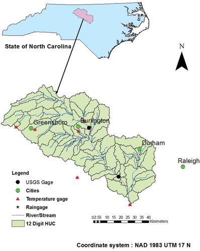
The Haw River watershed is situated at about longitude 35°35'E and latitude 10°40'N, in the north-central part of North Carolina (Fig. 1). It covers land in 10 counties (Forsyth, Guilford, Rockingham, Alamance, Orange, Chatham, Caswell, Durham, Randolph, Wake and Lee) and reaches almost 4000 km². The elevation ranges from 49 to 311 m with the mean elevation 180 m a.s. The length of the main stream is 177 km. The watershed experiences fairly wet climate with average annual precipitation varying from 1100 to 1200 mm. Historical extreme precipitation varies from 735 to 1694 mm. Temperatures in the winter normally range from 5 to 10°C, whereas summers are hot and humid with daytime temperatures in the range 24–33°C. Primary land cover in the watershed is forest (43%), other land-use classifications being agricultural (crop and pasture): 27%, urban development: 17%, and other: 13%. The Haw River is the longest tributary of Jordan Lake. It contributes 70–90% of the total surface inflow to the lake. At present Jordan Lake is the source for 3785.41 × 10⁶ litres of drinking water daily to the towns of Cary, Apex, Morrisville, northern Chatham County and the Wake County portion of Research Triangle Park. Almost all the water from the Haw River and tributaries flows directly into Jordan Lake, which is continuously under investigation for several water-related issues, including water availability, allocation, drought management and water quality (Tetra Tech 2003).

Figure 1. Location of the Haw River watershed in central North Carolina showing USGS streamflow gages and climate stations.

2.3 Data collection

Necessary input data for a SWAT simulation include topography, weather, land use, soil and management data. Topography data were obtained in the form of a digital elevation model (DEM) at 30 m resolution from the USGS Seamless Data Warehouse (http://nationalmap.gov/viewer.html). The cropland data layer (CDL) was used to develop land-use data for the watershed (USDA/NASS; http://www.nass.usda.gov/research/Cropland/SARS1a.htm). The State Soil Geographic Database (STATSGO) was used to create a soil database. Daily climatic data include precipitation, maximum and minimum air temperature, solar radiation, wind speed and relative humidity for each subwatershed. These climatic inputs can be entered from historical records or generated internally in SWAT using monthly climate statistics that are based on long-term weather records. Daily climatic data for a period of 59 years (1950–2009) were obtained from USDA to use as historical weather information for the model (USDA ARS http://www.ars.usda.gov/Research/docs.htm?docid=19390). Daily streamflow records were obtained from the USGS for the sites 02096500 (at Haw River) and 02096960 (at Bynum).

2.4 Hydrological simulation and calibration procedure

Watershed delineation was performed in such a way that the boundary of the subwatersheds match with the 12-digit hydrologic unit codes (HUCs) (Seaber et al. 1987). A total of 502 HRUs were created by ArcSWAT for the 57 subwatersheds. There are 19 USGS streamflow gage stations in the watershed. However, many of the stations lacked complete datasets for the entire simulation period. The model was calibrated and validated with stations that had continuous data for the study period and were able to represent the spatial heterogeneity of the watershed. Streamflow data at USGS gage 02096500 (drainage area 1570 km²) and USGS gage 02096960 (drainage area 3310 km²) were selected for calibration and validation. The entire simulation period was divided into a calibration period (2000–2009) and a validation period (1990–1999). SWAT version 2009 was calibrated manually using the Interactive SWAT application (i_SWAT) (Gassman et al. 2003). Calibration for water balance and stream flow was initiated by calibrating the overall water balance for average annual conditions. The Web-based Hydrograph Analysis Tool (WHAT), an automated digital filter technique, was used to separate the streamflow into two contributing components: surface runoff and baseflow. An overall estimate of 42% of baseflow was determined, which is in close agreement with the accepted range of groundwater contribution to streamflow for this region estimated by the USGS (Santhi et al. 2007).

Initial simulation was carried out by first using default values of all calibration parameters, which were later adjusted within their permissible ranges while matching simulation flow with the measured flow. Based on the literature and previously conducted research, nine widely-used flow calibration parameters were employed: curve number (CN), soil evaporation compensation factor (ESCO), baseflow alpha factor (ALPHA_BF), groundwater delay (GW_DELAY), deep aquifer recharge (RCHRG_DP), groundwater revap coefficient (REVAP), soil available water capacity (SOL_AWC), threshold water required in the shallow aquifer for baseflow to occur (GWQMN), and plant uptake compensation factor (EPCO). It was seen that the most sensitive parameter affecting the streamflow was CN followed by ESCO, SOL_AWC and REVAP. To assess the performance of any type of simulation model, there is an obvious need for some kind of statistical or computational indicators which can assist in the model evaluation. Four popularly used performance criterion were used to check SWAT’s ability to reproduce streamflow. These were the coefficient of determination (R²), Nash Sutcliffe efficiency (E), percent bias (PBIAS) and RMSE-observations standard deviation ratio (RSR). Model input parameters were continuously varied within the prescribed ranges during the calibration phase until simulated streamflow was within R² ≥ 0.5, E ≥ 0.5, ±15 < PBIAS < ±25 and 0 < RSR < 0.6. Model performances were classified as recommended by Moriasi et al. (2007).

2.5 Development of climate change scenarios

Climate models adopt quantitative methods to replicate the interactions of atmosphere, oceans, land surface and ice. To incorporate forecasted climatic information in the modeling set-up, the North American Climate Change Assessment Program (NARCCAP)’s high-resolution climate scenario data were used as a resource. There are several ways of conducting hydrological impact assessment due to climate change; for example, the delta change method (Jha and Gassman 2013a, Jha et al. 2013b), direct output of climate models (Takle et al. 2005, 2010), bias corrected output of climate models (Franczyk and Chang 2008, Jin and Sridhar 2012), statistical methods using weather generator, among others. This study used direct output of climate models assuming that the climate models are able to simulate future climate with a reasonable accuracy. Furthermore, contemporary data for the selected climate models were not available and so climate model performance could not be assessed with regard to the historical climate data. Daily information of dynamically downscaled climatic data from four climate models (GCM-RCM combinations) were used in the simulation, as follows:

• RCM3-CGCM3: Regional climate model version 3 driven by third generation coupled global climate model;

• RCM3-GFDL: Regional climate model version 3 driven by geophysical Fluid Dynamics Laboratory;

• HRM-HADCM3: Hadley regional Model 3 driven by Hadley Centre coupled model version 3; and

• CRCM-CGCM3: Canadian regional climate model driven by third generation coupled global climate model.

Relevant details of these climate models can also be found at the NARCCAP website (www.narccap.uca.edu). The four different model combinations allowed inspection of a broader range of possible changed climate conditions that might be prevalent in the region in the near future. The A2 emissions scenario, which depicts a very heterogeneous world based upon the underlying theme of self-reliance and preservation of local identities, was used in the study. This storyline assumes that economic development is primarily regionally oriented, and that per capita economic growth and technological change are more fragmented and slower than in the other storylines. Under this A2 emissions scenario, CO₂ concentrations for the middle and end of the 21st century are expected to be about 575 and 870 ppmv, respectively. Dynamic downscaling was performed on these data to obtain the watershed-scale information at a resolution of 50 km. The climatological baseline period used for the impact assessment was from 2040 to 2069. This time span is denoted as the mid-century. Climatic variables that were downscaled included daily maximum and minimum temperature, and daily precipitation. After the climatic data from the climate models had been processed, efforts were taken to import new climatic information into the SWAT model set-up which was already calibrated and validated. This was all done using the i_SWAT application which helped in storing and managing all the input data and the calibrated parameter set within a single database, thereby allowing us to modify the inputs, and the model was run from the same platform. SWAT was executed using observed historical climate (1980–2009) and future GCM-RCM projected climate (2040–2069). All comparisons (and percentage change calculations) were referenced to the baseline period (1980–2009). Change in precipitation was calculated by direct comparison of historical observations and projected data from the GCM-RCM. Changes in evapotranspiration and water yield were based on SWAT simulated results.

3 Results and discussions

3.1 Model calibration and validation

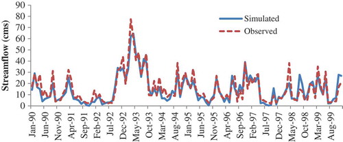
As noted earlier, nine influential parameters were selected based upon the literature; the most sensitive of these were CN, ESCO, SOL_AWC and GW_REVAP. Table 1 lists all the parameters that were calibrated to their final acceptable values. Figure 2 shows the comparison plot of historical monthly streamflow vs SWAT simulated monthly streamflow after the calibration process had been applied. The model tends to under-predict peak flow in some cases, as evident by visual inspection of the comparison (Fig. 2). However, the performance measured by the four statistical methods show a strong correlation. Similarly, Fig. 3 is the comparison plot for the validation period; during this simulation period, the model parameters were kept the same except for the climatic information. Simulated streamflow was found to match well with observed streamflow except for a few peaks. Table 2 displays the model efficiency during the calibration and validation phase.

Table 1. Calibration parameters and their final values used for the Haw River watershed.

Parameter	Range	Final value
Curve number (CN2)	30–98	Reduced by 10%
Soil evaporation compensation factor (ESCO)	0–1	0.88
Plant uptake compensation factor (EPCO)	0–1	0.05
Baseflow alpha factor (Alpha_BF)	0–1	0.3
Threshold depth of water in the shallow aquifer (GWQMN)	0–very high	5
Groundwater “revap” coefficient (GW_REVAP)	0.02–0.2	0.18
Groundwater delay time (GW_DELAY)	0–100	50
Deep aquifer percolation fraction (RCHRG_DP)	0–1	0.18
Soil available water capacity (SOL_AWC)	±0.04	+0.04

Table 2. Model efficiency for streamflow calibration and validation periods.

Station	Calibration period (2000–2009)				Validation period (1990–1999)
	R^2	E	PBIAS	RSR	R^2	E	PBIAS	RSR
Haw River near Bynum, NC	0 .90	0.90	−0.8%	0.32	0.89	0.88	8%	0.38
Haw River at Haw River, NC	0.87	0.86	9%	0.37	0.86	0.76	22%	0.49

Figure 2. Monthly flow calibration (2000–2009) for the Haw River watershed at Haw River, NC.

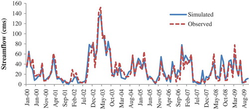
Figure 3. Monthly flow validation (1990–1999) for the Haw River watershed at Haw River at Haw River, NC.

Results indicated that about 60% of the annual rainfall is lost by evapotranspiration in the watershed. Surface runoff and baseflow contributed about 55% and 40% of the total water yield, respectively. Overall, it can be concluded that the calibrated model was able to replicate the watershed hydrology of the Haw River watershed very well.

3.2 Projected climate and impact assessment

3.2.1 Precipitation

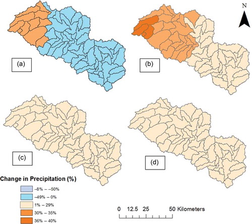
Under the baseline condition (1980–2009), average annual precipitation was found to vary between 1058 and 1179 mm with spatially an increasing gradient towards the south of the watershed (Fig. 4). Spatial analysis suggests an increase in average annual precipitation across all the subwatersheds under the HRM-HADCM3, RCM3-CGCM3 and RCM3-GFDL scenarios (Fig. 5(b)–(d)), while, under the CRCM-CGCM3 scenario, only the northern part is expected to receive more rainfall (Fig. 5(a)). One distinct feature in the comparison of spatial variation is that the areas receiving more rainfall under current conditions are expected to receive less rainfall in future, whereas comparatively dry areas will receive more rainfall.

Regarding the precipitation pattern, a steady increase in the rainfall amounts was observed on an annual basis for all model projections, except for the CRCM-CGCM3, which projected a 3% decrease. Other model combinations agreed on a wetter mid-century condition for the watershed, with the greatest increase in the HRM-HADCM3 projection (29% increase). A 38% decrease in the precipitation in the months of early fall (September and October) was observed in all the model scenarios in the mid-century with the greatest average decrease in the month of September. January to April exhibited a 30% increase in rainfall. December showed a 67% increase in rainfall amount under all the model scenarios in mid-century. Figure 6 shows the monthly precipitation projections on a spatial scale. Based on the analysis of the four climate models’ prediction of precipitation, it can be inferred that Haw River watershed is most likely to have wetter winters and springs under future climatic conditions.

Figure 4. Spatial distribution of precipitation in the Haw River watershed under the baseline scenario (1980–2009).

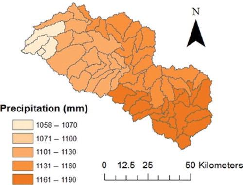
Figure 5. Percent change in mean annual precipitation (from baseline) for the mid-century under: (a) CRCM-CGCM3, (b) HRM-HADCM3, (c) RCM3-CGCM3, and (d) RCM3-GFDL.

3.2.2 Evapotranspiration

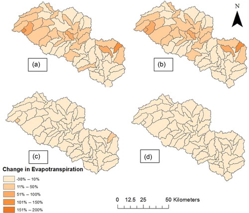
Evapotranspiration (ET) is considered to be major factor influencing the spatiotemporal availability of water but is often difficult to quantify, especially on a watershed scale. It was found that two of the four climate models, CRCM-CGCM3 and HRM-HADCM3, caused ET to increase with a respective magnitude of 12% and 11% from current conditions. Also, model combinations of RCM3-CGCM3 and RCM3-GFDL tend to agree on a mid-century decrease of ET by 11% and 6%, respectively. The ET was found to be more strongly correlated with temperature than precipitation. Increase in ET was consistent with the overall increase in projected temperature and vice versa. Of the four climate models used, CRCM-CGCM3 and HRM-HADCM3 projected an increase of 1.26°C and 1.9°C, respectively, in mean annual temperature in the mid-century, and the corresponding simulations of ET were found to increase by 82 and 71 mm, respectively. The RCM3-CGCM3 and RCM3-GFDL models projected a decrease in mean annual temperature by 0.21°C and 1.83°C, respectively, in the mid-century, which produced a decrease in ET by 39 mm and 75 mm, respectively. It is important to note that the effect of precipitation was also included in the overall simulation, but the predicted impact seemed to follow the direct relationship between temperature and ET. Our results were found consistent with similar studies where ET varied accordingly to air temperature (Abbaspour et al. 2009, Setegn et al. 2011). All the scenario combinations show ET values increasing for the months of late summer (July and August), which is when the plant water requirement is highest (Fig. 7).

Evapotranspiration showed a wide range of spatial variation under baseline conditions, from 289 to 857 mm on an average annual basis. The ET values were found to be higher in the parts of the watershed where the dominant land use is forest, whether deciduous or evergreen. Most rainfall is lost as ET because the major portion of the land use is forest. Generally the central part of the watershed is associated with a medium range of variation in the increase of the ET. The southern part of the watershed is mostly found to experience a decrease in ET under all model projections. Spatial variations of ET projected by the different model combinations can be observed in Fig. (8(a)–(d)).

Figure 6. Mean monthly precipitation for the baseline (1980–2009) and four climate model scenarios at mid-century (2040–2069).

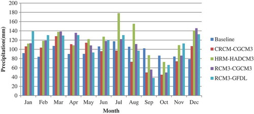
Figure 7. Mean monthly actual ET for the baseline (1980–2009) and four climate model scenarios at mid-century (2040–2069).

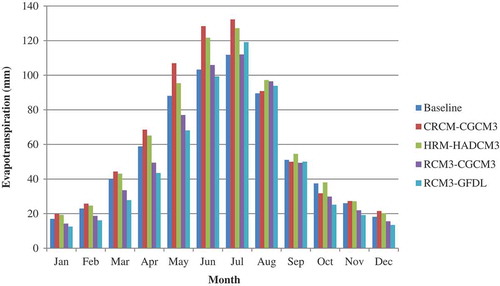
Figure 8. Percent change in mean annual ET (from baseline) for the mid-century under: (a) CRCM-CGCM3, (b) HRM-HADCM3, (c) RCM3-CGCM3, and (d) RCM3-GFDL.

3.2.3 Water yield

Water yield is the total water available for streamflow and is the sum of surface runoff and baseflow. Scenario results indicated that water yield would vary significantly in the mid-century. Average annual values of water yield were mostly found to increase except for the CRCM-CGCM3 model scenario.

Under current conditions, water yield, similar to evapotranspiration, has a wide range of spatial variation, from 179 to 674 mm on an annual basis. As expected, the portions of the watershed with a major land use of forest and agricultural practices have a lower range of water yield. With the exception of CRCM-CGCM3, all model combinations result in an increasing water yield in the mid-century (Fig. 9(a)–(d)). In general, the northern part of the watershed was found to have the most pronounced increase in water yield in future.

Figure 9. Percent change in mean annual water yield (from baseline) for the mid-century under: (a) CRCM-CGCM3, (b) HRM-HADCM3, (c) RCM3-CGCM3, and (d) RCM3-GFDL.

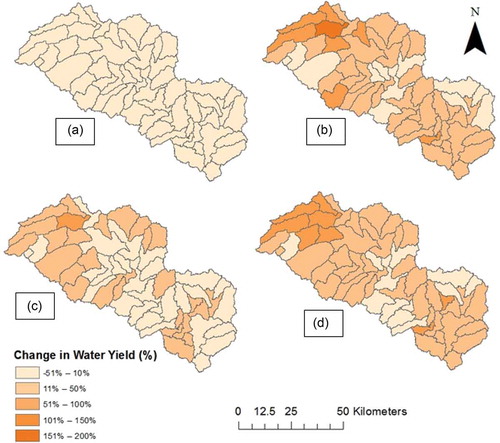
Further analysis revealed that mostly spring months (February, March, April and May) would experience 74% increase in the water yield in all the scenarios by mid-century (Fig. 10). It was noted that a pronounced increase in water yield was expected in May under all scenarios.

Figure 10. Mean monthly water yield for the baseline (1980–2009) and four climate model scenarios at mid-century (2040–2069).

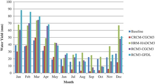
The direction of water yield changes followed the same trend as precipitation, although the changes in water yield are greater in magnitude than the precipitation changes. A possible interpretation could be the increase in surface runoff generation leading to increase in water yield in future.

3.2.4 Overall hydrological balance

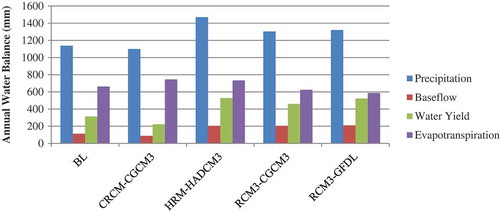
The hydrological balance of water movement is basically controlled by precipitation and evapotranspiration, which finally results in water yield. Figure 11 compares the average annual water balance components under the baseline and mid-century climate scenarios. The watershed is expected to receive 14% more rainfall on average, producing a corresponding 38% greater water yield, which infers that the Haw River watershed is expected to experience excess water. The increasing trend of surface runoff and groundwater discharge could result in major alterations in the quantity of water present at a particular area at any time, indicating that water resources management and decision making should be planned well in advance.

Figure 11. Annual water balance components under baseline and climate model scenarios in the mid-century (Note: BL represents “baseline” in this figure).

Table 3 summarizes the impacts assessment on the major water balance components of the watershed under the projected climate scenarios. The proportion of rainfall becoming runoff seems to increase in the mid-century climate scenarios with the exception of the CRCM-CGCM3 model scenario. The percentage of evapotranspiration from rainfall is reduced in almost all the scenarios despite the increase in rainfall, again except for the CRCM-CGCM3 scenario. This behaviour of the watershed under the changing climate could be attributed to the fact that there may be frequent occurrences of higher intensity rainfall that result in less retention of moisture in soil. Gradual increase in the proportion of rainfall becoming baseflow in the Haw River watershed is also noted mid-century in all the model scenarios except for CRCM-CGCM3. This different outcome was not clearly understood. The behaviour of the CRCM-CGCM3 model scenario might be explained by the underlying climate physics involved. Climate models replicate atmospheric phenomenon in various ways. This is a good reason to use multiple model ensembles to reduce uncertainties in predictions.

Table 3. Comparison of change in water balance components as % of precipitation (ppt) for IPCC A2 scenario for the mid-century under different model combinations.

Scenario	Precipitation (mm)	Water yield		Actual ET		Baseflow
		(mm & % of ppt.)		(mm & % of ppt.)		(mm & % of ppt.)
Baseline	1138	313	28	663	58	112	10
CRCM-CGCM3	1100	223	20	745	68	88	8
HRM-HADCM3	1470	528	36	734	50	203	14
RCM3-CGCM3	1304	460	35	624	48	204	16
RCM3-GFDL	1320	523	40	588	45	210	16

3.2.5 Implications for Jordan Lake

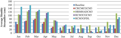
Analysis of average monthly streamflow at the watershed outlet (inflow to Jordan Lake) revealed that that the monthly streamflow is generally expected to increase in the mid-century, the climate change scenarios agreeing that there might be an 80% increase in the streamflow in spring months (February, March, April and May), with the greatest increase in May (107% increase; Fig. 12). Projections for the monthly streamflow follow the same trend as water yield, with the model combinations showing that there may be an increase in the amount of water flowing to Jordan Lake in the mid-century. Thus it could be inferred that Jordan Lake might be subject to floods in the mid-century.

Figure 12. Mean monthly streamflow comparison at the watershed outlet for the baseline and climate model scenarios.

3.2.6 Extreme event analysis

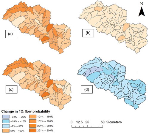
Changes in future flood and drought conditions were quantified using the daily simulated streamflow for each subwatershed. There is a general increase in the percentage of high flows occurring in the watershed in the mid-century, which indicates that, under changing climate, flooding conditions may be exacerbated. The RCM3-CGCM3 scenario suggests the most pronounced increase in percentage of peak discharge (up to 284%), followed by the CRCM-CGCM3 and HRM-HADCM3 scenarios. The RCM3-GFDL scenario simulation results demonstrate that there could be an increase as well as a decrease in the peak discharge above the 99th percentile, indicating less chance of the occurrence of extreme events. Upon further analysis of the spatial variation in the peak discharge, a clear trend was found that is indicative of a larger increase of peak flows in the northern part of the watershed (Fig. 13). This could be further correlated to the significant increase of water yield in the northern part of the watershed in the mid-century. It also reveals that the eastern part of the watershed is most likely to experience a reduction in peak flows under all the model scenarios. The urban land cover could be mostly termed safe as there was little increase in peak discharge in those areas. Figure 13(a)–(d)) shows change in peak discharge equal to or exceeding a 1% frequency from baseline to mid-century for the Haw River watershed under the different scenarios.

Figure 13. Percent change in stream discharge at 99th percentile (from baseline) for the mid-century under (a) CRCM-CGCM3, (b) HRM-HADCM3, (c) RCM3-CGCM3, and (d) RCM3-GFDL.

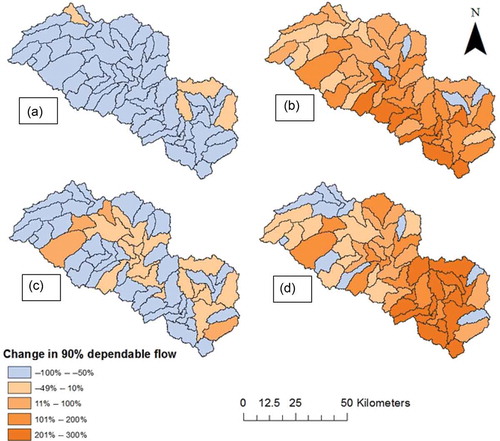
Assessment of dependable lean season flows along with their distribution in time is critical for planning and development of water supply management. Impact of climate change on the dependability of the water yield of the river system was analysed with respect to three levels of 90% dependability with the help of flow duration curves. A 90% probability level is considered safe to determine assured water supply. Figure 14(a)–(d)) displays the spatial variation of change of 90% dependable flow from baseline to mid-century. The results indicate that low flows have different trends under different scenarios. For the CRCM-CGCM3 and RCM3-CGCM3 scenarios the hydrological drought situation was aggravated as the discharge at the 10th percentile decreased by 86 and 62%, respectively, on average over the entire watershed. However, drought scenarios seem less probable under the RCM3-GFDL and HRM-HADCM3 scenarios, as the discharge at the 10th percentile increases by 96 and 92%, respectively, when averaged over the watershed. Under the CRCM-CGCM3 scenario, there is a constant decrease in the low flow pattern, with the central part of the watershed showing a high percentage of drought-like condition. The northern part of the watershed shows a reduction in low flows (90% dependability), whereas the southern part shows an increase in low flows. However, the trend over the whole watershed during the mid-century shows a general decrease in the low flow. The severest droughts could occur in the central-south part of the watershed, whereas the urban areas could be considered safe as there was not much reduction in the low flow situation in the cities.

Figure 14. Percent change in stream discharge at 10th percentile (from baseline) for the mid-century under (a) CRCM-CGCM3, (b) HRM-HADCM3, (c) RCM3-CGCM3, and (d) RCM3-GFDL.

4 Conclusions

A modeling set-up was developed using SWAT, four dynamically downscaled regional climate models, a GIS interface and other pertinent information and software to assess the impact of climate change on water distribution and availability in the Haw River watershed in North Carolina. All the climate models used, except CRCM-CGCM3, agree on a wetter mid-century (2040–2069) condition compared to the baseline (1980–2009), with the greatest increase in precipitation being observed in the HRM-HADCM3 projection (29% increase on an average annual basis). Water yield was found to follow the precipitation projection with pronounced increase under the projected climatic conditions. The greatest increase in water yield was found in the HRM-HADCM3 scenario (69% increase), while CRCM-CGCM3 predicts a 29% decrease in total water yield. Evapotranspiration was found to decrease or increase depending on the different model combinations. There was an increasing trend (on average by 8%) from the baseline for the months of late summer (July and August). Analysis of the average monthly streamflow at the watershed outlet (which serves as a the main source of water for Jordan Lake) shows that there might be considerable increase in streamflow in spring.

Some limitations of the study presented here include, but are not limited to: (1) the non-availability of contemporary climate data which prohibits checking of the climate models’ accuracy of predicting climate, and (2) the future climate scenarios did not consider changes in land use on the hydrological processes. These issues should be investigated in future studies to encompass a broader scale of impact assessment with reduced uncertainties. Future research should focus on investigating the effects of population growth on water yield and including open water evaporation in model calculations.

Disclosure statement

No potential conflict of interest was reported by the authors.

References

- Abbaspour, K.C., et al., 2009. Assessing the impact of climate change on water resources in Iran. Water Resources Research, 45, W10434. doi:10.1029/2008WR007615
- Abdo, K.S., et al., 2009. Assessment of climate change impacts on the hydrology of Gilgel Abay catchment in Lake Tana Basin, Ethiopia. Hydrological Processes, 23, 3661–3669.
- Arnold, J.G., et al., 1998. Large area hydrologic modeling and assessment part I: model development. Journal of the American Water Resources Association, 34, 73–89. doi:10.1111/j.1752-1688.1998.tb05961.x
- Christensen, S.N., et al., 2004. The effects of climate change on the hydrology and water resources of the Colorado River basin. Climatic Change, 62 (1–3), 337–363. doi:10.1023/B:CLIM.0000013684.13621.1f
- Diffenbaugh, N.S., et al., 2005. Fine-scale processes regulate the response of extreme events to global climate change. Proceedings of the National Academy of Sciences of the United States of America, 102 (44), 15774–15778. doi:10.1073/pnas.0506042102
- Ficklin, D.L., Stewart, I.T., and Maurer, E.P., 2013. Climate change impacts on streamflow and subbasin-scale hydrology in the Upper Colorado River Basin. PLoS ONE, 8 (8), e71297. doi:10.1371/journal.pone.00
- Franczyk, J. and Chang, H., 2008. The effects of climate change and urbanization on the runoff of the Rock Creek basin in the Portland metropolitan area, Oregon, USA. Hydrological Processes, 23 (6), 805–815. doi:10.1002/hyp.7176
- Gassman, P.W., et al., 2003. The i_SWAT software package: a tool for supporting SWAT watershed applications. In: 2nd International SWAT Conference Proceedings. Texas Water Resources Institute, 229–234. Available from: http://swat.tamu.edu/docs/swat/conferences/2003/2ndswatconfproceeding.pdf
- Gleick, P.H. and Chalecki, E.L., 1999. The impacts of climatic changes for water resources of the Colorado and Sacramento–San Joaquin river basins. Journal of the American Water Resources Association, 35, 1429–1441. doi:10.1111/j.1752-1688.1999.tb04227.x
- IPCC (Intergovernmental Panel on Climate Change). 2007. Climate change 2007: Impacts, adaptation and vulnerability. Contribution of Working Group II to the Fourth Assessment Report of the Intergovernmental Panel on Climate Change. Cambridge University Press.
- IPCC (Intergovernmental Panel on Climate Change). 2009. Climate change: The physical science basis. Contribution of Working Group I to the Fourth Assessment Report of the Intergovernmental Panel on Climate Change. Cambridge: Cambridge University Press. Available from: http://www.ipcc.ch/ipccreports/ar4-wg1.htm
- IPCC (Intergovernmental Panel on Climate Change). 2012. Managing the risks of extreme events and disasters to advance climate change adaptation. Cambridge: A Special Report of Working Groups I and II of the Intergovernmental Panel on Climate Change. Available from: http://www.ipcc-wg2.gov/SREX/images/uploads/SREX-All_FINAL.pdf
- Jha, M.K., et al., 2006. Climate change sensitivity assessment on Upper Mississippi River Basin streamflows using SWAT. Journal of the American Water Resources Association, 42, 997–1015. doi:10.1111/j.1752-1688.2006.tb04510.x
- Jha, M.K. and Gassman, P.W., 2013a. Changes in hydrology and streamflow as predicted by modeling experiment forced with climate models. Hydrological Processes. doi:10.1002/hyp.9836
- Jha, M.K., Gassman, P.W., and Panagopoulos, Y., 2013b. Regional changes in nitrogen loadings in the Upper Mississippi River Basin under predicted mid-century climate. Journal of Regional Environment Change. doi:10.1007/s.10113-013-05539-y
- Jha, M.K., et al., 2004. Impact of climate change on stream flow in the Upper Mississippi River Basin: a regional climate model perspective. Journal of Geophysical Research, 109, D09102. doi:10.1029/2003JD003686
- Jin, X. and Sridhar, V., 2012. Impacts of climate change on hydrology and water resources in the Boise and Spokane River Basins. Journal of the American Water Resources Association, 48 (2), 197–220. doi:10.1111/j.1752-1688.2011.00605.x
- Moriasi, D.N., et al., 2007. Model evaluation guidelines for systematic quantification of accuracy in watershed simulations. Transactions of the ASABE, 50 (3), 885–900. doi:10.13031/2013.23153
- Neitsch, S.L., et al., 2005. Soil and Water Assessment Tool theoretical documentation: version 2005. Temple, TX: USDA-ARS Grassland, Soil and Water Research Laboratory. Available from: http://swatmodel.tamu.edu/documentation/
- Santhi, C., et al., 2007. Regional estimation of baseflow for the conterminous United States by hydrologic landscape regions. Journal of Hydrology, 35, 139–153.
- Seaber, P.R., Kapinos, F.P., and Knapp, G.L., 1987. Hydrologic Units Maps. Reston, VA: US Geological Survey Water-Supply Paper 2294.
- Setegn, S.G., et al., 2011. Impact of climate change on the hydroclimatology of Lake Tana Basin, Ethiopia. Water Resources Research, 47, W04511.
- Stewart, I.T., Cayan, R.D., and Dettinger, D.M., 2004. Changes in snowmelt runoff timing in western North America under a “business as usual” climate change scenario. Climate Change, 62 (1–3), 217–232. doi:10.1023/B:CLIM.0000013702.22656.e8
- Takle, E.S., Jha, M.K., and Anderson, C.J., 2005. Hydrological cycle in the Upper Mississippi River Basin: 20th century simulations by multiple GCMs. Geophysical Research Letters, 32, L18407. doi:10.1029/2005GL023630
- Takle, E.S., et al., the NARCAP Team, 2010.Streamflow in the Upper Mississippi River Basin as simulated by SWAT driven by 20th Century contemporary results of global climate models and NARCCAP regional climate models. Meteorologische Zeitschift, 19 (4), 341–346. doi:10.1127/0941-2948/2010/0464
- Tetra Tech, 2003. B. Everett Jordan Lake TMDL Watershed Model Development. A report to the North Carolina Division of Water Quality, Department of Environment and Natural Resources. Durham, NC: Triangle J Council of Governments. Available from: www.tcog.org
- US Global Change Research Program, 2009. Global climate change impacts in the United States. Available from: http://downloads.globalchange.gov/usimpacts/pdfs/climate-impacts-report.pdf