Hybrid modelling approach to prairie hydrology: fusing data-driven and process-based hydrological models

Abstract

Much of the prairie region in North America is characterized by relatively flat terrain with many depressions on the landscape. The hydrological response (runoff) is a combination of the conventional runoff from the contributing areas and the occasional overflow from the non-contributing areas (depressions). In this study, we promote the use of a hybrid modelling structure to predict runoff generation from prairie landscapes. More specifically, the Soil and Water Assessment Tool (SWAT) is fused with artificial neural networks (ANNs), so that SWAT and the ANN module deal with the contributing and non-contributing areas, respectively. A detailed experimental study is performed to select the best set of inputs, training algorithms and hidden neurons. The results obtained in this study suggest that the fusion of process-based and data-driven models can provide improved modelling capabilities for representing the highly nonlinear nature of the hydrological processes in prairie landscapes.

Editor D. Koutsoyiannis; Associate editor L. See

Résumé

Une grande partie de la région des Prairies en Amérique du Nord est caractérisée par un terrain relativement plat avec de nombreuses dépressions. La réponse hydrologique (ruissellement) est la combinaison de l'écoulement classique à partir des zones qui contribuent et du trop-plein occasionnel des zones ne contribuant pas (dépressions). Dans cette étude, nous favorisons l'utilisation d'une structure de modélisation hybride pour prévoir la génération de ruissellement des paysages des Prairies. Plus précisément, le modèle Soil and Water Assessment Tool (SWAT) a été fusionné avec des réseaux de neurones artificiels (RNA), de sorte que les modules SWAT et RNA gèrent respectivement les domaines contributifs et non contributifs..Une étude expérimentale détaillée a été effectuée pour sélectionner le meilleur jeu de données d'entrée, les algorithmes d’entraînement et les neurones cachés. Les résultats obtenus dans cette étude suggèrent que la fusion de modèles basés sur les processus et dirigés par les données peut améliorer la capacité de la modélisation à représenter la nature fortement non linéaire des processus hydrologiques dans les paysages des Prairies.

Key words:

• prairie hydrology
• unconventional runoff generation
• hybrid modelling
• Soil and Water Assessment Tool (SWAT)
• artificial neural network (ANN)

Mots clefs:

• hydrologie des prairies
• génération de ruissellement non conventionnelle
• modélisation hybride
• Soil and Water Assessment Tool (SWAT)
• réseaux de neurones artificiels (RNA)

1 INTRODUCTION

The prairie region of North America covers a vast area of west-central Canada and north-central USA. The prairie region is characterized by flat terrain with many depressions; therefore, it does not possess a well-defined drainage system and much of the land drains into small wetlands called potholes. This creates a complex hydrological phenomenon, where the response of the watershed is highly dependent on the details within the landscape, including the location and the linkage among the potholes (Van Der Kamp et al. 2003). For the Canadian prairies, Agriculture and Agri-Food Canada (AAFC) identified the extent of non-contributing areas as those that do not contribute runoff to the watershed outlet for an event of 2-year return period (Prairie Farm Rehabilitation Administration 2008). These non-contributing areas, however, are varying in time. During below-average precipitation conditions, many of the potholes dry up, while in wet periods, they expand, merge and start contributing to the runoff process. It has been noted that the contribution of potholes in the formation of total runoff can vary greatly between seasons and/or hydrological years (Shaw 2010). High seasonality and inter-annual variability is a prominent feature in prairie regions. Moreover, Fang et al. (2008) noted that extreme hydrological events, well below- or well above-average annual runoff events, are a normal component of the historical flow regime in the prairie region. For instance, the most recent drought in the Canadian prairies occurred from 1999–2004 (Lemmen et al. 2008), which was followed by a set of extreme flooding events in 2010 and 2011.

Accurate estimation of streamflow is important for reducing the effects of extreme events as well as for proper management of water resources systems. Prediction of hydrological processes for the prairie landscape, however, remains challenging due to incomplete understanding of some physical processes within potholes as well as the nonlinearity in the relationship between the fraction of a contributing area and the water storage in the basin (Spence 2007, Shaw 2010). In addition, Shook et al. (2011) noted that the storage of water in the prairie potholes may cause ‘memory’ in the system, where the response of the system at any time depends on the history of inputs and outputs. Due to these difficulties, conventional hydrological models have considerable limitations for the prairie landscape. Still, there is a tendency for crude simplification of the hydrological processes in prairie regions. For instance, Wen et al. (2011) assumed that non-contributing areas were completely isolated and fixed over time. On the other hand, some studies assumed the entire basin, including potholes, was contributing to streamflow for all events (e.g. Shrestha et al. 2012). Similarly, Sophocleous et al. (1999) applied the Soil and Water Assessment Tool (SWAT) model in an area of 3375 km² in the Rattlesnake Creek basin, Kansas, USA. They identified 62% of the watershed as non-contributing area, which never contributes to the main stream.

There are, however, some attempts to represent the pothole processes in hydrological models in a dynamic manner. Spence (2010) compared the dynamic contributing area of depression storage to the variable source area concept and advised a ‘fill-and-spill’ mechanism to consider the activation of the non-contributing area. Although fill-and-spill theory sounds physically appealing, there are major difficulties in implementing the idea in large-scale hydrological models. Fang et al. (2008) applied the Cold Regions Hydrological Model (CRHM) to assess the hydrological process within a small watershed (3.85 km²) with one pothole. However, the suggested method is computationally expensive and could be difficult to implement in a large-scale watershed (with numerous potholes). Liu et al. (2008) made an effort to include a riparian wetland module in the Soil and Water Assessment Tool (SWAT). They applied the developed module in a 53-km² wetland located in southern Ontario, Canada. The results showed that the new module can improve the quality of the output from the SWAT model; however, the model was not fully validated due to limitations of the observed data.

We argue that due to the importance of dynamic non-contributing area in determining the total response of the catchment and the difficulties associated with the fill-and-spill hypothesis at larger scales, there is a need for alternative approaches to enhance the capability of conventional models in simulating discharge in prairie catchments. Accordingly, we suggest a hybrid modelling framework to handle dynamics and activation modes of non-contributing areas in a large prairie watershed (9360 km²), located in Saskatchewan, Canada. This hybrid model uses the SWAT model to represent the hydrological response of contributing areas and an artificial neural network (ANN) model to characterize the dynamics of the non-contributing areas based on the residual of the SWAT simulation for contributing areas. The objective of this paper is to demonstrate this model fusion, to discuss the technical issues around model development, and to examine its applicability in real-world modelling problems.

The remainder of this paper is organized as follows. In Section 2, the SWAT, ANN, and hybrid SWAT-ANN modelling approaches are briefly introduced. In Section 3, the watershed characteristics and dataset used are discussed. Section 4 describes the model development procedures and the evaluation methods used for comparing model performance. Section 5 evaluates the results obtained from the SWAT, ANN, and the hybrid SWAT-ANN models, and finally, Section 6 provides concluding remarks.

2 METHODS

2.1 SWAT model

The Soil and Water Assessment Tool (SWAT) is a physically-based hydrological model that simulates the various hydrological processes of a watershed (Arnold et al. 1998, Neitsch et al. 2011). The SWAT model was developed by the US Department of Agriculture - Agricultural Research Service and has been used in numerous watersheds in the USA and around the world (Gassman et al. 2007). The model has been used for simulating runoff response (e.g. Lévesque et al. 2008) and nutrient transport (e.g. Panagopoulos et al. 2007). In particular, it has been applied in the prairies (Sophocleous et al. 1999, Shrestha et al. 2012). As described in Arnold et al. (1998), SWAT simulates the hydrological cycle of a watershed by partitioning it into a number of sub-basins that are further grouped into hydrological response units (HRUs)—lumped areas within a sub-basin that are comprised of unique combinations of land cover, soil type and slope. Information required for each sub-basin includes climate, HRU, size of ponds/wetlands, groundwater and river reaches (Neitsch et al. 2011).

In general, the SWAT model runs on a daily time step and was intended to model large agricultural watersheds. The model simulates the hydrology of a watershed in two steps: the land phase and routing phase (Neitsch et al. 2011). The land phase controls the amount of water contributed to the main channel reach in each sub-basin. Hydrological processes are computed separately for each HRU of the sub-basin. Surface runoff is computed using either the modified curve number method (CN) (USDA Soil Conservation Service 1972) or the Green-Ampt method (Green and Ampt 1911). Potential evapotranspiration is estimated using one of three different methods that include Penman-Monteith (Monteith 1965), Priestley-Taylor (Priestley and Taylor 1972) and Hargreaves (Hargreaves et al. 1985) approaches. The actual evaporation from soils and plants is estimated as described by Ritchie (1972). The SWAT model also simulates impoundments such as reservoirs, wetlands and ponds. Ponds and wetlands are water storage elements within a sub-basin to intercept the surface runoff within the sub-basin. Baseflow is modelled by partitioning groundwater into a two-aquifer system (shallow and deep) (Arnold et al. 1993). The routing phase controls movement of water through the stream network to the watershed outlet. Streamflow routing is performed based on either the variable storage coefficient method (Williams 1969) or the Muskingum routing method (Cunge 1969).

2.2 ANN model

Artificial neural networks (ANNs) are a set of data-driven system identification methods that are designed to mimic the operation of biological nervous systems. ANNs are often used to model complex relationships between observations, particularly when physical processes mapping the inputs to outputs are not known in advance. There are many different kinds of ANNs (Guez et al. 1988); however, the multilayer preceptor (MLP) with the back-propagation learning algorithm is the most widely used type in modelling and prediction of water resources variables (Maier and Dandy 2000). The MLP used in this study consists of three layers: an input layer, a hidden layer and output layer. In such a configuration of the ANN model input data are presented to the input layer. Each neuron receives all inputs from the input layer through weighted connections. The weighted inputs are then summed and a bias term is added, followed by a transfer function (usually linear, logistic and hyperbolic tangent) to produce the output of the layer. The output from this layer then passes through the next layers until the network output is produced at the output layer. It has been shown that such a network configuration has universal capability (Hornik et al. 1989).

The benefits of using this ANN architecture have been well recognized in the literature (Abrahart et al. 2012). So far, ANNs have been applied in a wide range of hydrological modelling problems (Solomatine and Xue 2004, Altunkaynak 2007, Coulibaly 2010), including runoff prediction (e.g. Elshorbagy et al. 2000), evapotranspiration estimation (e.g. Kişi 2006, Izadifar and Elshorbagy 2010), non-Darcy flow in porous media (e.g. Nazemi et al. 2006) and sediment load modelling (e.g. Talebizadeh et al. 2010), among others. Although it has been shown that MLPs are useful in describing complex dynamic systems (Srivastava et al. 2006), the performance of MLP models is sensitive to input datasets, the network training method, and the network structure selected (Elshorbagy et al. 2010). Moreover, MLP parameters increase substantially by increasing the number of hidden neurons. Therefore, a rigorous procedure is required for identifying the appropriate inputs, hidden layer structure and training algorithm for a given problem.

2.3 Hybrid of SWAT and ANN models

The terminology of hybrid modelling indicates an integrated modelling structure that may include more than one model based on different modelling paradigms. In this regard, a limited number of hybrid hydrological models are available in the literature. These have included the integration of ANNs with conceptual models in rainfall–runoff modelling (Chen and Adams 2006, Jain and Srinivasulu 2006), the combination of semi-distributed process-based and data-driven models (Corzo et al. 2009), the combination of ANNs and the kinematic wave approach (Chua and Wong 2010), as well as sediment load estimation (Talebizadeh et al. 2010). Earlier, Zhang (2003) tested a hybrid autoregressive integrated moving average (ARIMA) and ANN model over three kinds of time series in such a way that ARIMA was used to simulate the linear pattern of the data and ANNs were trained using the residuals of the ARIMA model that contain information about the nonlinear pattern. Zhang (2003) concluded that the combined model improved forecasting more than either model used independently. Corzo et al. (2009) have proposed hybrid modelling as a baseflow separation technique based on a modular architecture that takes into account the various flow regimes. They reported improved predictions from a modular approach that takes into account different flow components much better than global models. Recently, Corzo et al. (2009) tested a hybrid modelling framework of semi-distributed process-based (IHMS-HBV) and data-driven models in streamflow simulation. They found improved model performance in the context of flow forecasting by combining a semi-distributed process-based model (IHMS-HBV) and a data-driven model. They replaced sub-basin conceptual and river routing components of IHMS-HBV with data-driven models.

As noted earlier, the nonlinear overflow response from non-contributing areas in prairie regions is due to dynamic fill-and-spill patterns of large networks of potholes with extremely complicated connectivity (Spence et al. 2010, Phillips et al. 2011, Shook et al. 2011, Ehsanzadeh et al. 2012). The hydrological response in prairie regions is a combination of a conventional runoff process from contributing areas and unconventional overflow generation from non-contributing areas (potholes). Equation (1) defines the partition of total streamflow at the watershed outlet as the sum of water yield from contributing areas and non-contributing areas.

(1)

where F_total(t) is total measured flow, F_c(t) is flow from contributing areas, and F_nc(t) is flow from non-contributing areas. For the hybrid model and following equation (1), SWAT is used to represent the runoff generation from contributing areas and the ANN model is used to represent the nonlinear overflow generation from the non-contributing areas.

Considering the SWAT model, the generated runoff from contributing areas can be described as:

(2)

where F_SWATc(t) is the simulated flow from contributing areas using the SWAT model, and E(t) is the error associated with SWAT while simulating contributing areas. Substituting equation (2) in equation (1) with some rearrangement, equation (3) can be formulated:

(3)

Equation (3) shows that the residuals of the SWAT model for contributing areas contain information on overland flow from non-contributing areas, as well as the error initiated from the SWAT model itself. Accordingly, an ANN model can be trained, based on residuals of the SWAT model, to handle the flow from non-contributing areas. In such a configuration, SWAT simulations can provide a proxy about the instantaneous wetness condition of the catchment that determines the extent of total flow contributed by potholes. In the operational mode, therefore, SWAT simulations can be plugged into the ANN model as an exogenous input in conjunction with hydroclimatic variables. Using such a topology, the total flow at any given time can be estimated as the sum of the SWAT simulation for contributing areas and the ANN model that filters the SWAT simulations using other variables to provide a notion of runoff generated from potholes. Figure 1 shows the schematic representation of the proposed hybrid model. The systematic procedure for developing this hybrid model as well as SWAT- and ANN-only models is introduced and discussed in Section 4. We also compared the performance of the hybrid model with SWAT- and ANN-only structures in Section 5.

Fig. 1 Framework of the SWAT-ANN hybrid modelling system.

3 CASE STUDY

3.1 Study area

The study was conducted on the Moose Jaw River watershed (Fig. 2), which is bounded by 49–51°N latitudes and 104–107°W longitudes. It is the largest tributary to the Qu'Appelle River with a gross drainage area of 9360 km² of which about 70% is used for agricultural purposes, in particular crop production. The elevation of the watershed ranges from 877 to 530 m a.m.s.l. The slope of the watershed varies depending upon the geology of the area: ranging from steep slopes in the Missouri Coteau (along the western edge) to a level topography in the Regina Plains (throughout most of the watershed). Annual precipitation in the basin over the past 90 years has varied from a minimum of 200 mm/year to a maximum of 600 mm/year, of which 20% falls as snow in the winter months, 20% occurs during spring, 45% falls as rain during the summer, and the remaining 15% occurs during the autumn (Saskatchewan Watershed Authority 2005). The 30-year (1971–2000) mean annual precipitation at Moose Jaw is 365 mm, of which 115.5 mm occurs mostly as snow in winter; the 30-year annual average air temperature at Moose Jaw is 4°C, with daily temperature ranges from a maximum of 41.7°C (6 August 1949) to a minimum of −45.6°C (23 January 1943) (Environment Canada 2009).

Fig. 2 The prairie pothole region and location of the study watershed at Moose Jaw (05JE006) in Canada.

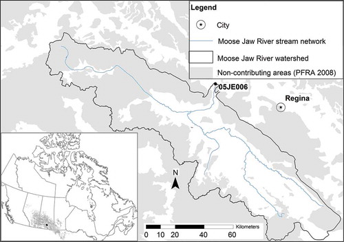
The watershed is located in an area of diverse soil types ranging from heavy clay soils in the east to gravelly sandy soils in the west. Frozen soils and wind redistribution of snow develop over the winter, and snowmelt and meltwater runoff normally occur in the early spring, with the peak basin streamflow usually in the second half of April. The spring snowmelt runoff contributes 80% or more of the annual surface runoff for prairie streams (Gray and Landine 1988). On average, only 3% of annual precipitation reaches the watershed outlet as flow in the Moose Jaw River. The majority is returned to the atmosphere either through evaporation from wetlands and the ground surface or through transpiration from plants. A small percentage (less than 5%) recharges the groundwater system.

3.2 Available data

Both spatial and point datasets used in this study are freely available from different sources. Detailed land-cover data and digital elevation model (DEM) data were obtained from GeoBase Canada (http://www.geobase.ca/) at resolutions of 1:250 000 and 1:50 000, respectively. The detailed soil data at a scale of 1:1 000 000 were obtained from Agriculture and Agri-Food Canada (Shields et al. 1991), respectively. A map of effective and non-contributing areas in the watershed was also obtained from this source (Prairie Farm Rehabilitation Administration 2008). The measured streamflow at the outlet of the catchment was obtained from the Hydrometric Database (HYDAT), produced by Water Survey of Canada. The gauging station (ID 05JE006) is located at 50°24ʹ1.2″N and 105°23ʹ52.3″W. Daily rainfall, snow, maximum and minimum temperature data were acquired from the Environment Canada database for the weather station at Moose Jaw (climate, ID 4015320) (50°20ʹN; 105°33ʹW), which is located within the watershed.

In this study, the daily weather data from January 1987 to May 1997 was used for model development purposes including a ‘warm-up’ period (January 1987–December 1989), calibration period (January 1989–December 1994) and validation period (January 1995–May 1997). The use of a warm-up period minimizes the potential adverse effect of poorly estimated initial state variables such as soil water content (Zhang et al. 2007). An unseen dataset from January 1980 to December 1984 was used to test the generalization capability of the developed models.

3.3 Model evaluation methods

Different types of goodness-of-fit statistics (equations (4)–(8)) were used to assess the performance of the developed models. These measures are the root mean squared error (RMSE), the Nash-Sutcliffe coefficient of efficiency (NSE), the mean error (ME), the mean absolute error (MAE), Pearson’s correlation coefficient (R), and the Bayesian information criterion (BIC). The root mean square error (RMSE) measures the overall agreement between the observed and predicted datasets, with:

(4)

where O_i is the observed value at time i, P_i is the predicted value at time i, n is the total number of observations. It is more sensitive to large errors and ranges between zero and positive infinity.

The Nash-Sutcliffe coefficient of efficiency (NSE) is given by:

(5)

where is the mean observed error. The NSE value ranges from –∞ to 1. A value of 1 represents a perfect fit between predicted and observed values and 0 is interpreted to mean that the model is no better than a prediction that gives the mean of the observations for all time steps.

The mean error (ME) (equation (6)), measures the bias and has no upper and lower bound.

(6)

Mean absolute error (MAE) has also been used to evaluate model performance and is given by:

(7)

The other statistical measure that was used in the current study was the Pearson correlation coefficient (R):

(8)

where is the mean of the predicted value.

The Bayesian information criterion (BIC) is a likelihood measure and it penalizes models that have many parameters:

(9)

where m is the number of parameters of the model and MSE is the mean of the squared errors. Thus the first term of the BIC index measures the goodness-of-fit of the model, while the second term penalizes the model based on the number of the parameters.

4 MODEL DEVELOPMENT

4.1 SWAT model set-up

The SWAT model was developed for the entire Moose Jaw River watershed and further adjusted to connect only the contributing areas to the stream network. In brief, the hydrological components of SWAT model for the entire Moose Jaw River watershed (SWAT-only) were configured using the ArcSWAT interface for SWAT2009 (Neitsch et al. 2011). The DEM data with a resolution of 1:50 000 were used to define stream networks and delineate the watershed boundary and the internal sub-watersheds draining to the Moose Jaw River gauging station (05JE006). The land-use and soil maps were used to define the HRUs. In the set-up, potential evapotranspiration was estimated following Hargreaves (Hargreaves et al. 1985) and snowmelt was estimated using a temperature index method (Neitsch et al. 2011). Non-contributing areas were represented in the SWAT-only model using SWATs “pond” option. This allows runoff water to be initially stored and then overflow into the stream network during extreme events. For each sub-basin, a pond can be implemented with a user-defined fraction of the sub-basin draining to it. In this study, the fractional area of each sub-basin not draining into the stream network was identified based on a non-contributing area map obtained from Agriculture and Agri-Food Canada (Prairie Farm Rehabilitation Administration 2008). The pond characteristics, including surface area and volume in each sub-basin, were estimated using ArcGIS and the DEM.

Once the set-up of the SWAT-only model for the entire watershed was completed, the model was calibrated for a daily time step using the measured streamflow record (1989–1994). A combination of manual and automatic calibration using ParaSol (van Griensven and Meixner 2007) methods was performed to obtain optimum parameter values (Table 1). The calibration parameters were selected based on sensitivity analysis and results of previous studies in snow-dominated watersheds (Abbaspour et al. 2007, Lévesque et al. 2008). The Latin hypercube one-factor-at-a-time (LH-OAT) method (Morris 1991) was used for the sensitivity analysis of the SWAT-only model parameters. The highly sensitive parameters that affect flow, i.e. CN2, SMTMP, TIMP, GW_DELAY, ESCO, SOL_AWC, ALPHA_BF, SFTMP, CH_N, SMFMX, SMFMN, and SURLAG (see Table 1 for definitions), were modified to improve the agreement between the simulated and observed daily flow. The feasible range (Abbaspour et al. 2007) and the optimum parameter values obtained for the Moose Jaw River watershed are presented in Table 1.

Table 1 Optimum parameter values for SWAT model for whole watershed.

Parameter	Expected range (Abbaspour et al. 2007) Min Max		Default value	Optimum value
SCS curve number (CN2)	−35%	+35%	Varies	+3
Soil evaporation compensation (ESCO)	0	1	0.95	0.78
Surface runoff lag coefficient (SURLAG)	0.5	10	4	0.75
Groundwater delay time (GW_DELAY)	10	100	31	29
Baseflow factor for bank storage (Alpha_BF)	0	1	0.048	0.48
Manning’s n for the main channel (CH_N)	0.01	0.2	0.014	0.11
Soil available water (SOL_AWC)	−0.04	+0.04	Varies	+0.01
Snowmelt base temperature (SMTMP)	−3	3	0.5	1.5
Snowfall temperature (SFTMP)	−3	3	1	0.6
Maximum melt factor (SMFMX)	0	10	4.5	3.0
Minimum melt factor (SMFMN)	0	10	4.5	1.0
Snow pack temperature lag factor (TIMP)	0.01	1	1	0.3

The calibrated SWAT model for the entire watershed was further adjusted to only simulate the generated runoff from contributing areas (F_SWATc). To do so, the calibrated SWAT-only model parameters for the entire watershed remain unchanged, but the outflow from ponds (that hold the precipitation falling on non-contributing areas) was systematically prevented from being routed as part of surface runoff. This was achieved by making the storage of ponds large values (i.e. preventing overflow from ponds), and setting the seepage from ponds to zero. To confirm the adjustment, the outflow through overspill and seepage from ponds was checked for the simulation period of this project. The ponds in the SWAT model never reached their capacity to overspill and seepage from ponds was confirmed to be zero. Under such a configuration, the whole precipitation falling on the non-contributing area portion is not allowed to contribute to the stream networks. Accordingly, the simulation using the adjusted SWAT model (after adjusting ponds to not contribute) represents only the portion of water generated from contributing areas.

4.2 Input selection for ANN models

Artificial neural networks were used to describe the total streamflow from the whole watershed (ANN-only) as well as the flow from non-contributing areas (equation (3)). The Neural Network Toolbox in MATLAB was used to develop the ANN models. Considering the climatic condition of our case study, four groups of hydroclimatic variables, i.e. rainfall, temperature, snowpack and snowmelt, can be the drivers of hydrological response. Snowmelt is computed based on the degree-day method (Anderson 1976), in which temperature is a key variable affecting snowmelt estimation. We also considered 30-day accumulated rainfall depth as a potential driver of the hydrological response. Srivastava et al. (2006) suggested the use of 30-day accumulated rainfall in ANN modelling as an indicator of the contribution of groundwater to the streamflow. If the appropriate time lags of these variables are found, then they can be considered as the inputs to ANN models. To find the suitable time lags and a set of efficient input variables, we performed a correlation analysis, followed by an initial model performance assessment using a unique ANN structure but different input combinations. First, based on considering different daily lags of each of the hydroclimatic variables, a correlation analysis was performed to identify the lags with highest correlation with the target (total streamflow in the case of ANN-only for the entire watershed or SWAT residuals of contributing areas ANN model for potholes, see equation (3)). The results of this analysis are summarized in Fig. 3. The considered lags cover delay from zero to several days between the input and the target. The analysis revealed large lags between input and the target variables. This has physical justification due to the prairie region landscape of a near flat slope and interception of the flow by potholes which delays the streamflow response.

Fig. 3 Correlation between different input variables and their lags with target: (a) the entire watershed; and (b) the non-contributing areas.

Input variables and lags that have higher correlation with the target were selected and further combined with other highly correlated variables to investigate the effect of different input combinations. Several input combinations were investigated; only input combinations with better model performance are presented in Table 2 below. To do so, a hidden layer with only two neurons was linked to various combinations of the scaled input variables. Two neurons are selected because that is the simplest ANN structure that could make this mapping. The number of hidden neurons was then further fine-tuned (see Section 4.3). The MSE was used to train the neural network using the Levenberg-Marquardt (LM; Levenberg 1944, Marquardt 1963) training algorithm. The effect of the training algorithm on the quality of modelling will be addressed in Section 4.4.

Table 2 Different input combinations and the performance of ANN model for non-contributing areas and entire watershed based on Pearson correlation coefficient (the selected input combinations are highlighted in bold).

Input combinations (entire watershed)	R	Input combinations (non-contributing areas)	R
SP-34	0.61	SP-19	0.50
SP-34, SP-35	0.64	SP-19, SP-20	0.51
SP-34, SP-35, SP-36	0.71	SP-19, SP-20, SP-21	0.53
SP-34, SP-35, SP-36, SP-37	0.73	SP-19, SM-6	0.52
SP-34, SP-35, SP-36, SP-37, SM-5	0.85	SP-19, SM-6, SM-7	0.51
SP-34, SP-35, SP-36, SP-37, SM-5, SM-6	0.86	SP-19, SM-6, SM-7, SM-8	0.55
SP-34, SP-35, SP-36, SP-37, SM-5, SM-6, SM-7	0.88	SP-19, SM-8, RF-142	0.52
SP-34, SP-35, SP-36, SP-37, SM-5, SM-6, SM-7, RF-260	0.88	SP-19, RF-142, RF-160	0.53
SP-34, SP-35, SP-36, SP-37, SM-5, SM-6, SM-7, RF-260, TMP-84	0.87	SP-19, RF-142, TMP-3	0.51
SP-34, SP-35, SP-37, SM-5, SM-6, SM-7, RF-260, TMP-84	0.85	SP-19, SM-8,	0.82
SP-34, SP-35, SP-36, SP-37, SM-5, SM-6, SM-7, RF-260, TMP-85	0.86	SP-19, SM-8, , , ARF	0.88
SP-34, SP-37, SM-6, SM-7, ARF	0.87	SP-19, SM-8, RF-142	0.52
SP-34, SP-35, SP-37, SM-5, SM-6, SM-7	0.82		0.71
SP-34, SM-5, RF-260, TMP-84	0.75	,	0.76

SP-34: snow pack input delayed by 34 days; SM-5: snowmelt input delayed by 5 days; TMP-3: temperature input delayed by 3 days; RF-142: rainfall input delayed by 142 days; ARF: 30 days accumulated rainfall; : simulated flow for contributing areas using SWAT model.

According to the correlation analysis (Fig. 3) and the analysis of model performance for different input combinations (Table 2), the most effective input combination for ANN modelling for the entire watershed (with the target of total observed flow) includes the snow pack with 34-day lag (SP-34), snow pack with 37-day lag (SP-37), snowmelt with 5-day lag (SM-5) and 7-day lag (SM-7), and 30-day accumulated rainfall (ARF). For the ANN model structure for the entire watershed the variables that have information about the groundwater system contribution are snowpack (important during winter and spring periods) and accumulated rainfall (important during summer period). The snowmelt variables contain information about the fast response component.

Similarly, the most parsimonious input combination for the ANN model developed for the non-contributing areas (with a target of total observed flow minus SWAT simulation for contributing area) are snowpack with 19-day lag (SP-19), snowmelt with 8-day lag (SM-8), current simulated flow for the contributing areas (F_SWATc), simulated flow for the contributing areas with 1-day lag (F_SWATc-1), and 30-day accumulated rainfall (ARF). In such an ANN model structure, the SWAT result from contributing areas contains information about the instantaneous wetness condition of the catchment including both groundwater and overland flow contributions. Nonetheless, it should be noted that other variables, such as snowmelt, snowpack and accumulated rainfall, should also be considered in conjunction with SWAT simulations to handle the extreme conditions response of non-contributing areas. As shown in Table 2 below, model performance has been improved when snowmelt, snowpack and accumulated rainfall variables are added on top of SWAT simulations from contributing areas. Inclusion of temperature as an input variable does not bring a significant improvement in model performance (see Table 2) as information about temperature is already incorporated through the snowmelt variable (estimated using degree-day method).

4.3 Number of hidden neurons

A detailed sensitivity analysis was conducted to obtain the most efficient number of hidden neurons based on the structural complexity, robustness of training, simulation accuracy, and predictive uncertainty. For both ANN models for the whole catchment and non-contributing areas, we sequentially increased the number of hidden neurons from one to 10. Each ANN model was retrained 1000 times using the LM algorithm. The justification for increasing the structural complexity was investigated using the BIC criterion (equation (9)). Robustness of training and overall accuracy was analysed by monitoring the discrepancy and the median of E_RMS in 1000 training attempts. Finally, predictive uncertainty was observed by looking at the simulation envelope. All these post-training investigations were performed during the validation phase.

Based on this analysis, it was revealed that in the case of modelling the entire watershed, having more than five hidden neurons results in sensitive model parameters. Sensitive model parameters are those that (a) were largely distributed in the feasible parametric space; and (b) considerably varied in each calibration trial. This threshold is three neurons in the case of the ANN model for non-contributing areas. Based on Fig. 4, the overall (i.e. median) improvement in RMSE and BIC from four to five hidden neurons may not be significant; nonetheless, the ANN model with five neurons is justifiable for the entire watershed because the variability in convergences is decreased. Figure 5 shows the analysis of the predictive uncertainty for the ANN model with four or five hidden neurons. Based on comparing the prediction envelope, the options with five hidden neurons have lower predictive uncertainty during the validation period particularly for the wet summer of 1997.

Fig. 4 Performance measures of 1000 ANN models with four and five hidden neurons for modelling the entire watershed: (a) root mean square error (RMSE); and (b) Bayesian information criterion (BIC). The performance measures are calculated during the validation phase.

Fig. 5 Predictive uncertainty for ANN model developed for the entire watershed during the validation period: (a) four; and (b) five hidden neurons.

Similar analysis was performed for the ANN model trained for the non-contributing area. In this case, instead of the measured streamflow, SWAT residuals (observed minus SWAT from contributing areas) are the target of the ANN model. Therefore, the performance analysis is inherently related to the ANN model and the uncertainty associated with the SWAT model was ignored. This is justifiable as the intention of this analysis is to select the hidden neurons for simulating the residuals of the SWAT model. Our analysis showed that increasing the number of hidden neurons beyond three is not justifiable based on BIC criterion and results in sensitive model parameters. However, configuring the ANN with three neurons improves the error measures and variability in convergence over two neurons (Fig. 6). Figure 7 compares the range of model predictions based on 1000 ANN models trained with two and three hidden neurons. In this case the ANN model with three hidden neurons exhibit lower predictive uncertainty over the structure than with two hidden neurons.

Fig. 6 Performance measures of 1000 ANN models with two and three hidden neurons for modelling the SWAT residuals: (a) root mean square error (RMSE); and (b) Bayesian information criterion (BIC). The performance measures are calculated during the validation phase.

Fig. 7 Predictive uncertainty for ANN model developed for the non-contributing areas during the validation period: (a) two; and (b) three hidden neurons.

4.4 Selection of training algorithm

Training ANNs can be a difficult optimization problem due to the complexity of the mapping between inputs and outputs, as well as the large number of free parameters. These issues can result in a highly complicated fitness landscape with several local optima. There are several training algorithms suggested for training neural networks. The training efficiency can be evaluated using the time and the robustness of the training through multiple calibration trials. Here the behaviours of two training algorithms, namely LM and Bayesian regulation (BR) (Mackay 1992) were analysed using the variations in the time of convergence as well as the associated BIC measures. The ANNs with selected number of hidden neurons (see Section 4.3) were re-trained 1000 times using LM and BR algorithms. The results are illustrated in Fig. 8. Considering the ANN model of non-contribution areas with three neurons, it was revealed that, on average, the LM method can result in faster training; however, the robustness of training is significantly degraded. Considering relatively quick convergence (approximately 3 s) in the case of training the ANN for non-contributing areas, BR was used for re-training the ANN model with three neurons fitted to SWAT residuals. Regarding the training of the ANN model for the entire watershed, the LM algorithm can result in strictly faster and robust training, although BR is more likely to identify solutions with better fitness. By analysing the simulation bound, it was also noticed that solutions obtained by the BR algorithm may result in considerably wider prediction bounds during the validation phase, when compared to the LM simulations.

Fig. 8 Time complexity and the robustness of training using Bayesian regulation (BR) and Levenberg–Marquardt (LM) methods obtained based on 1000 re-calibration: (a) and (b) ANN model for non-contributing areas using three neurons; and (c) and (d) ANN model using five neurons for the entire watershed.

5 RESULTS AND DISCUSSION

The results of model performance evaluation are presented in Table 3 for calibration, validation and testing phases using the best simulation obtained through 1000 re-training. The statistical comparison showed that the hybrid SWAT-ANN model outperforms individual SWAT and ANN models in all three modelling phases.

Table 3 Statistical indices of SWAT, ANN and Hybrid model performance for training, validation and testing periods.

	Calibration (1989–1994)			Validation (1995–1997)			Testing (1980–1984)
	SWAT	ANN	Hybrid	SWAT	ANN	Hybrid	SWAT	ANN	Hybrid
RNSE	5.5	3.73	2.84	7.89	7.24	4.76	5.04	6.35	4.57
NSE	0.68	0.81	0.85	0.78	0.84	0.89	0.74	0.62	0.81
ME	−1.65	−0.26	−0.38	0.45	0.51	0.08	−0.94	0.24	0.21
MAE	2.24	1.55	1.11	2.77	2.54	1.77	1.76	2.17	1.25
BIC	3060	2450	2011	1587	1592	1313	2905	3394	2851

The streamflow dataset was segmented into winter and non-winter flows in order to assess the relative performance of individual models over various seasons (see Table 4). All performance evaluation measures (Table 4) suggest that the hybrid model seems to be performing better (higher NSE and lower RMSE, ME, MAE, and BIC) than the individual models for non-winter as well as winter flows. The Nash-Sutcliffe coefficient of efficiency (NSE; Table 4) suggests that non-winter flows are adequately simulated by all three models. However, the NSE measure suggests that the ANN model did not adequately simulate low flows.

Table 4 Statistical indices of SWAT, ANN and Hybrid model performance for separated high and low flow conditions.

	High flow (non-winter)						Low flow (winter)
	Calibration			Validation			Calibration			Validation
	SWAT	ANN	Hybrid	SWAT	ANN	Hybrid	SWAT	ANN	Hybrid	SWAT	ANN	Hybrid
RMSE	9.61	5.95	5.81	15.55	11.52	8.57	1.49	2.43	1.37	2.01	2.81	1.33
NSE	0.75	0.90	0.91	0.81	0.89	0.94	0.60	−0.04	0.67	0.40	−0.22	0.72
ME	−4.45	−0.40	−2.81	3.98	3.36	1.35	−0.39	−0.47	0.01	−0.71	−0.36	−0.08
MAE	6.79	2.66	3.95	8.64	6.49	5.17	0.52	1.23	0.43	0.88	1.37	0.74
BIC	716	590	583	517	472	428	650	1252	545	529	719	297

To investigate the quality of modelling visually, the simulated daily flows are plotted against the corresponding measured values. Figure 9 shows the scatter plot for calibration and validation periods for the hybrid model, as well as the SWAT and ANN models for the whole watershed. As can be observed, the SWAT and ANN models have some bias during the high and low flows, respectively. This is particularly noticeable during the validation period. The SWAT-ANN hybrid model, however, merges the benefits of both individual models and considerably decreases the modelling biases of the SWAT and ANN models during the low and high periods. Figure 10 compares the simulated flows obtained using the best SWAT, ANN and hybrid SWAT-ANN modelling options. A better fit is provided by the hybrid structure compared to the individual models for the testing period.

Fig. 9 Simulated vs observed flow forcalibration and validation periods: (a) SWAT model; (b) ANN model; and (c) ANN-SWAT hybrid.

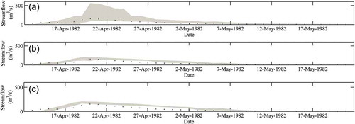
Fig. 10 Simulated streamflow of SWAT, ANN and hybrid SWAT-ANN models for the years: (a) 1982; (b) 1994; (c) 1996; and (d) 1997.

It has been widely recognized that the behavioural parameters of hydrological models change if one alters objective functions (Wagener et al. 2004). It is also preferable to select an identifiable model for prediction, in which optimal solutions are clustered in a small neighbourhood in the fitness landscape. We used a sampling/visualization study (see Pryke et al. 2007, Nazemi et al. 2008) to analyse the trade-off between MSE and mean absolute error (MAE) criteria and the identifiability of the associated optimal solutions in the ANN model for the non-contributing area. In brief, the ANN model with three neurons configured for non-contributing areas was re-trained using MSE as the objective function for 1000 times. For each trial, both MAE and MSE measures corresponding to the best parametric set were calculated. Figure 11(a) shows the trade-offs between the MSE and MAE measures. The grey, black stars and black dots show the whole results as well as the best 1% training samples based on MSE and MAE criteria, respectively. There is a clear trade-off between MSE and MAE, showing that, on the Pareto front, improving MSE would result in degrading the MAE and vice versa.

To investigate the parametric identifiability of the calibrated models based on MSE and MAE criteria, we measured the distance between the optimal solutions in the parametric space using multidimensional scaling or MDS, the approach outlined by Nazemi et al. (2008). In brief, MDS is a statistical method to visualize dissimilarities in data. The objective of MDS here is to reflect the dissimilarities between the optimal parametric sets in a two-dimensional space so the patterns and clusters within the solutions can be extracted. In MDS the original space is mapped in an abstract two-dimensional space (such as the principal coordinates) in a way that the relative distances between solutions in the original and projected spaces remain unchanged. This has been done by considering the Euclidian distance measures, in both original and principal coordinate spaces. Figure 11(b) shows the results of this analysis. The top 1% MSE solutions are quite sparse in the parametric landscape showing considerable lack of identifiability. In contrast, the best 1% solutions based on MAE criterion are rather concentrated on an identifiable parametric neighbourhood within the whole parametric landscape. This suggests that the MAE measure identifies a less sensitive ANN model for non-contributing area. This result was furthermore confirmed by quantifying the predictive uncertainty during the testing phase. First, the whole parametric sets (obtained based on 1000 recalibrations) were used to simulate the hydrological response. Then, only the best 1% solutions based on the MSE and MAE criteria were used to obtain the overflow from the non-contributing areas. Figure 12 shows that the simulation results based on the top 1% MAE solutions have a thinner prediction range compared with the top 1% MSE solutions during the most extreme event of the testing period.

Fig. 11 The trade-off between MSE (black stars) and MAE (black dots) criteria, and the resulting variations in the optimal parametric space for ANN model of non-contributing area with three hidden neurons.

Fig. 12 Predictive uncertainty in the SWAT-ANN hybrid model in the generalization period: (a) entire parametric set; (b) 1% best model parameters based on MSE; and (c) 1% best model parameters based on MAE.

6 SUMMARY AND CONCLUSION

Runoff generation in prairie regions exhibits a combined flow response resulting from conventional runoff processes in contributing areas as well as the occasional overflows from non-contributing areas (potholes). Although, the current process-based hydrological models can sufficiently represent the key hydrological mechanisms of the contributing areas, they have difficulty describing the unconventional hydrological responses from the non-contributing areas. This is due to the lack of physical understanding of the related fill-and-spill process, as well as the complexity and dynamic nature of the connection between the potholes spread over prairie landscapes.

In this study, a hybrid SWAT-ANN model was suggested, in which the SWAT model describes the runoff generation in contributing areas and the ANN model models the overflow from potholes. The selected structure was used to describe the daily hydrological response in the Moose Jaw River watershed, Saskatchewan, Canada. The investigation showed that a careful analysis is required to configure the ANN models for modelling the total streamflow response as well as the overflow from non-contributing areas. A detailed experimental study was performed to select the best input combinations, the optimal number of hidden neurons as well as training algorithm; and to address the efficiency, robustness, and identifiability of ANN models. It was shown that the hybrid SWAT-ANN model is capable of exploiting the strength of process-based and data-driven modelling approaches in a unified structure. The results revealed that the hybrid model outperforms the individual models with improved performance measures for calibration, validation and testing periods. Moreover, it was revealed that the individual models have certain biases. In particular, it was shown that the SWAT model cannot accurately describe high flows by ignoring the dynamics of non-contributing areas and representing the total response as a conventional hydrologic process. In contrast, the ANN model exhibited considerable error during the low and average periods by neglecting the physical processes that govern conventional runoff generation. The hybrid model, however, was able to describe the extreme conditions better than both individual models.

It was found, however, that there could be a significant trade-off when the hybrid model is in the optimal condition (see Fig. 11). This means that in order to improve one error measure, others should decline. It was also revealed that the optimal solutions might be quite sparse in the fitness landscape, which can hinder the application of the model in real-world assessment studies due to the predictive uncertainty, as well as the lack of parametric identifiability. For the selected case study, it was shown that selecting the representative ANN model parameters based on the MAE criterion results in a more identifiable model with better generalization capability; nevertheless, different results might be obtained in other watersheds. As a final remark, it is worth mentioning that ANNs can be potentially embedded as an internal module in the SWAT model to deal with non-contributing areas in a more physically-based manner. More studies, therefore, are suggested to improve the representation of runoff generation in prairie regions using process-based and data-driven modelling paradigms.

Disclosure Statement

No potential conflict of interest was reported by the author(s).

Acknowledgments

We thank the reviewers for their constructive comments that have helped improve the paper.

Additional information

Funding

The authors would like to thank the Province of Saskatchewan Go Green Fund and the Canada Excellence Research Chair in Water Security at the University of Saskatchewan for financial support for this work.

REFERENCES

- Abbaspour, K.C., et al., 2007. Modelling hydrology and water quality in the pre-alpine/alpine Thur watershed using SWAT. Journal of Hydrology, 333 (2–4), 413–430. doi:10.1016/j.jhydrol.2006.09.014
- Abrahart, R.J., et al., 2012. Two decades of anarchy? Emerging themes and outstanding challenges for neural network river forecasting. Progress in Physical Geography, 36 (4), 480–513. doi:10.1177/0309133312444943
- Altunkaynak, A., 2007. Forecasting surface water level fluctuations of lake van by artificial neural networks. Water Resources Management, 21 (2), 399–408. doi:10.1007/s11269-006-9022-6
- Anderson, E.A., 1976. A point energy and mass balance of a snow cover. NOAA Technical Report NWS-19, US Department of Commerce, Washington, DC.
- Arnold, J.G., Allen, P.M., and Bernhardt, G., 1993. A comprehensive surface-groundwater flow model. Journal of Hydrology, 142, 47–69. doi:10.1016/0022-1694(93)90004-S
- Arnold, J.G., et al., 1998. Large area hydrologic modelling and assessment part I: model development. Journal of the American Water Resources Association, 34 (1), 73–89. doi:10.1111/j.1752-1688.1998.tb05961.x
- Chen, J. and Adams, B.J., 2006. Integration of artificial neural networks with conceptual models in rainfall-runoff modelling. Journal of Hydrology, 318 (1–4), 232–249. doi:10.1016/j.jhydrol.2005.06.017
- Chua, L.H.C. and Wong, T.S.W., 2010. Improving event-based rainfall–runoff modelling using a combined artificial neural network–kinematic wave approach. Journal of Hydrology, 390 (1–2), 9–107.
- Corzo, G.A., et al., 2009. Combining semi-distributed process-based and data-driven models in flow simulation: a case study of the Meuse river basin. Hydrology and Earth System Sciences, 13, 1619–1634. doi:10.5194/hess-13-1619-2009
- Coulibaly, P., 2010. Reservoir computing approach to Great Lakes water level forecasting. Journal of Hydrology, 381, 76–88. doi:10.1016/j.jhydrol.2009.11.027
- Cunge, J.A., 1969. On the subject of a flood propagation computation method (Musklngum method). Journal of Hydraulic Research, 7 (2), 205–230. doi:10.1080/00221686909500264
- Ehsanzadeh, E., et al., 2012. On the behaviour of dynamic contributing areas and flood frequency curves in North American Prairie watersheds. Journal of Hydrology, 414–415, 364–373. doi:10.1016/j.jhydrol.2011.11.007
- Elshorbagy, A., Simonovic, S.P., and Panu, U.S., 2000. Performance evaluation of artificial neural networks for runoff prediction. Journal of Hydrologic Engineering, 5 (4), 424–427. doi:10.1061/(ASCE)1084-0699(2000)5:4(424)
- Elshorbagy, A.A., et al., 2010. Experimental investigation of the predictive capabilities of data driven modelling techniques in hydrology—Part 1: concepts and methodology. Hydrology and Earth System Sciences, 14, 1931–1941. doi:10.5194/hess-14-1931-2010
- Environment Canada, 2009. Canadian climate normals 1971-2000 [online]. Available from: http://www.climate.weatheroffice.ec.gc.ca/climate_normals/index_e.html. [Accessed: 10 December 2011].
- Fang, X., et al., 2008. Drought impacts on Canadian prairie wetland snow hydrology. Hydrological Processes, 22 (15), 2858–2873. doi:10.1002/hyp.7074
- Gassman, P.W., et al., 2007. The soil and water assessment tool: historical development, applications, and future research directions. Transactions of the ASABE, 50 (4), 1211–1250. doi:10.13031/2013.23637
- Gray, D.M. and Landine, P.G., 1988. An energy-budget snowmelt model for the Canadian Prairies. Canadian Journal of Earth Sciences, 25, 1292–1303. doi:10.1139/e88-124
- Green, W.H. and Ampt, G.A., 1911. Studies on soil physics, 1. The flow of air and water through soils. Journal of Agricultural Sciences, 4, 11–24.
- Guez, A., Protopopsecu, V., and Barhen, J., 1988. On the stability, storage capacity, and design of nonlinear continuous neural networks. IEEE Transactions on Systems, Man, and Cybernetics, 18 (1), 80–87. doi:10.1109/21.87056
- Hargreaves, G.L., Hargreaves, G.H., and Riley, J.P., 1985. Agricultural benefits for Senegal River Basin. Journal of Irrigation and Drainage Engineering, 111 (2), 113–124. doi:10.1061/(ASCE)0733-9437(1985)111:2(113)
- Hornik, K., Stinchcombe, M., and White, H., 1989. Multilayer feedforward networks are universal approximators. Neural Networks, 2 (5), 359–366. doi:10.1016/0893-6080(89)90020-8
- Izadifar, Z. and Elshorbagy, A., 2010. Prediction of hourly actual evapotranspiration using neural networks, genetic programming, and statistical models. Hydrological Processes, 24, 3413–3425. doi:10.1002/hyp.7771
- Jain, A. and Srinivasulu, S., 2006. Integrated approach to model decomposed flow hydrograph using artificial neural network and conceptual techniques. Journal of Hydrology, 317 (3–4), 291–306. doi:10.1016/j.jhydrol.2005.05.022
- Kişi, Ö., 2006. Evapotranspiration estimation using feed-forward neural networks. Nordic Hydrology, 37 (3), 247–260. doi:10.2166/nh.2006.010
- Lemmen, D., et al., 2008. From impacts to adaptation: Canada in a changing climate 2007. Ottawa: Natural Resources Canada.
- Levenberg, K., 1944. A method for the solution of certain problems in least squares. The Quarterly of Applied Mathematics, 2, 164–168.
- Lévesque, É., et al., 2008. Evaluation of streamflow simulation by SWAT model for two small watersheds under snowmelt and rainfall. Hydrological Sciences Journal, 53 (5), 961–976. doi:10.1623/hysj.53.5.961
- Liu, Y.B., Yang, W., and Wang, X., 2008. Development of a SWAT extension module to simulate riparian wetland hydrologic processes at a watershed scale. Hydrological Processes, 22 (16), 2901–2915. doi:10.1002/hyp.6874
- Mackay, D.J.C., 1992. A practical Bayesian framework for backpropagation networks. Neural Computation, 4, 448–472. doi:10.1162/neco.1992.4.3.448
- Maier, H.R. and Dandy, G.C., 2000. Neural networks for the prediction and forecasting of water resources variables: a review of modelling issues and applications. Environmental Modelling & Software, 15 (1), 101–124. doi:10.1016/S1364-8152(99)00007-9
- Marquardt, D., 1963. An algorithm for least squares estimation of nonlinear parameters. Journal of the Society for Industrial and Applied Mathematics, 11 (2), 431–441. doi:10.1137/0111030
- Monteith, J.L., 1965. Evaporation and the environment. In the state and movement of water in living organisms. 19th Symposia of the Society for Experimental Biology. Cambridge University Press, London, UK, p. 205–234.
- Morris, M.D., 1991. Factorial sampling plans for preliminary computational experiments. Technometrics, 33, 161–174. do i:10.1080/00401706.1991.10484804
- Nazemi, A.-R., Hosseini, S.M., and Akbarzadeh-T, M.-R., 2006. Soft computing-based nonlinear fusion algorithms for describing non-Darcy flow in porous media. Journal of Hydraulic Research, 44 (2), 269–282. doi:10.1080/00221686.2006.9521681
- Nazemi, A.R., et al., 2008. On the quality of multi-objective calibration results in conceptual rainfall-runoff models. In Proceedings of the European Conference on Flood Risk Management: Research into Practice, FloodRisk 2008, 30 September –2 October, Oxford, UK.
- Neitsch, S.L., et al., 2011. Soil and water assessment tool (SWAT) user’s manual: version 2009. Temple, TX: U.S. Department of Agriculture, Agricultural Research Service, Grassland, Soil, and Water Research Laboratory.
- Panagopoulos, I., Mimikou, M., and Kapetanaki, M., 2007. Estimation of nitrogen and phosphorus losses to surface water and groundwater through the implementation of the SWAT model for Norwegian soils. Journal Soils Sediments, 7 (4), 223–231. doi:10.1065/jss2007.04.219
- Phillips, R.W., Spence, C., and Pomeroy, J.W., 2011. Connectivity and runoff dynamics in heterogeneous basins. Hydrological Processes, 25, 3061–3075.
- Prairie Farm Rehabilitation Administration, 2008. Prairie farm rehabilitation administration (PFRA) watershed project–- areas of non-contributing drainage. Canada: Agriculture and Agri-Food Canada.
- Priestley, C.H.B. and Taylor, R.J., 1972. On the assessment of surface heat flux and evaporation using large-scale parameters. Monthly Weather Review, 100, 81–92. doi:10.1175/1520-0493(1972)100<0081:OTAOSH>2.3.CO;2
- Pryke, A., Mostaghim, S., and Nazemi, A., 2007. Heatmap visualization of population based multi objective algorithms. In: S. Obayashi, et al. eds. Evolutionary multi-criterion optimization. Berlin: Springer, 361–375. doi:10.1007/978-3-540-70928-2_29
- Ritchie, J.T., 1972. A model for predicting evaporation from a row crop with incomplete cover. Water Resources Research, 8, 1204–1213. doi:10.1029/WR008i005p01204
- Saskatchewan Watershed Authority, 2005. Background report: Assiniboine River watershed. Regina: Assiniboine Watershed. Technical committee, 123.
- Shaw, D.A., 2010. The influence of contributing area on the hydrology of the prairie pothole region of North America. Thesis (PhD). Department of Geography, University of Saskatchewan, Saskatoon, Canada.
- Shields, J.A., et al., 1991. Soil Landscapes of Canada—Procedures Manual and User’s Handbook—1991. LRRC Contribution Number 88-29, Land Resource Research Centre, Research Branch, Agriculture Canada, Ottawa. 74.
- Shook, K.R., et al., 2011. Memory effects of depressional storage in Northern Prairie hydrology. Hydrological Processes, 25 (25), 3890–3898. doi:10.1002/hyp.8381
- Shrestha, R.R., Dibike, Y.B., and Prowse, T.D., 2012. Modeling climate change impacts on hydrology and nutrient loading in the Upper Assiniboine Catchment. JAWRA Journal of the American Water Resources Association, 48 (1), 74–89. doi:10.1111/j.1752-1688.2011.00592.x
- Solomatine, D.P. and Xue, Y., 2004. M5 model trees and neural networks: application to flood forecasting in the upper reach of the Huai River in China. Journal of Hydrologic Engineering, 9 (6), 491–501. doi:10.1061/(ASCE)1084-0699(2004)9:6(491)
- Sophocleous, M.A., et al., 1999. Integrated numerical modelling for basin-wide water management: the case of the Rattlesnake Creek basin in south-central Kansas. Journal of Hydrology, 214, 179–196. doi:10.1016/S0022-1694(98)00289-3
- Spence, C., 2007. On the relation between dynamic storage and runoff: a discussion on thresholds, efficiency, and function. Water Resources Research, 43 (12), 1944–7973. doi:10.1029/2006WR005645
- Spence, C., 2010. A paradigm shift in hydrology: storage thresholds across scales influence catchment runoff generation. Geography Compass, 4, 819–833. doi:10.1111/j.1749-8198.2010.00341.x
- Spence, C., et al., 2010. Storage dynamics and streamflow in a catchment with a variable contributing area. Hydrological Processes, 24, 2209–2221. doi:10.1002/hyp.7492
- Srivastava, P., McNair, J.N., and Johnson, T.E., 2006. Comparison of process-based and artificial neural network approaches for streamflow modelling in an agricultural watershed. Journal of the American Water Resources Association (JAWRA), 42 (3), 545–563. doi:10.1111/j.1752-1688.2006.tb04475.x
- Talebizadeh, M., et al., 2010. Uncertainty analysis in sediment load modelling using ANN and SWAT model. Water Resources Management, 24, 1747–1761. doi:10.1007/s11269-009-9522-2
- USDA Soil Conservation Service, 1972. National engineering handbook section 4 hydrology. Chapters 4–10. Washington, DC: U.S. Government Printing Office.
- Van Der Kamp, G., Hayashi, M., and Gallen, D., 2003. Comparing the hydrology of grassed and cultivated catchments in the semi-arid Canadian prairies. Hydrological Processes, 17, 559–575. doi:10.1002/hyp.1157
- van Griensven, A. and Meixner, T., 2007. A global and efficient multi-objective autocalibration and uncertainty estimation method for water quality catchment models. Journal of Hydroinformatics, 9 (4), 277–291. doi:10.2166/hydro.2007.104
- Wagener, T., Howard, S.W., and Hoshin, V.G., 2004. Rainfall-runoff modelling in gauged and ungauged catchments. England: Imperial College Print.
- Wen, L., et al., 2011. Reconstructing sixty year (1950-2009) daily soil moisture over the Canadian Prairies using the variable infiltration capacity model. Canadian Water Resources Journal, 36 (1), 83–102. doi:10.4296/cwrj3601083
- Williams, J.R., 1969. Flood routing with variable travel time or variable storage coefficients. Transactions of the ASAE, 12 (1), 100–103. doi:10.13031/2013.38772
- Zhang, G.P., 2003. Time series forecasting using a hybrid ARIMA and neural network model. Neurocomputing, 50, 159–175. doi:10.1016/S0925-2312(01)00702-0
- Zhang, X., Srinivasan, R., and Hao, F., 2007. Predicting hydrologic response to climate change in the Luohe river basin using the SWAT model. American Social Agricultural Biologic Engineering, 50 (3), 901–910.