Seasonal climate patterns and their influence on calibration of the Hargreaves-Samani equation

Abstract

Annual patterns in climate parameters were studied to evaluate how these influence the quality of reference evapotranspiration (ETo) estimates obtained from the Hargreaves-Samani (HS) equation, since the method only uses the measured temperature directly. The work evaluates how these patterns can be used to improve the HS ETo estimates. Ten-year moving averages from a set of California Irrigation Management Information System (CIMIS) stations were used to evaluate the relationships between solar radiation (R_s), temperature (T) and ETo. The results indicate that T treads behind solar radiation and its value peaks some 25 days later. Thus, the main irrigation season in the Mediterranean climate (1 May–30 September) can be divided into three phases: increasing R_s and T; decreasing R_s with increasing T; and decreasing R_s and T. Non-univocal annual cycles were observed between R_s and T, ETo and R_s, and ETo and T. These annual patterns result in important seasonal changes in the ratio between the HS and Penman-Monteith (FAO PM) ETo estimates. The changes are particularly important during the irrigation season, where the FAO PM initially calculates greater ETo values than the HS methodology, and from the end of May to early September, where the HS equation overestimates the ETo values (by 17 mm, or 3%). These patterns obtained from 2000–2009 data were used to calibrate and improve HS ETo estimates at new sites for the 2010–2011 period. Calibration based on the proposed seasonal region-wide FAO PM/HS ETo ratios improved both the bias (decreased from 0.40 to 0.36 mm d^-1) and r² (increased from 0.67 to 0.87) of the ETo estimates for the irrigation season. The proposed methodology can be easily applied to other regions, even when the existing weather stations are sparse.

Editor Z.W. Kundzewicz

Résumé

Le but de ce travail est d’étudier les modèles annuels des variables climatiques et d’évaluer la façon dont ils influencent la qualité des estimations de l’évapotranspiration de référence (ET_o) obtenues à partir de l’équation de Hargreaves Samani (HS), puisque cette méthode n’utilise que la température mesurée directement. Le travail évalue comment ces modèles peuvent être utilisés pour améliorer les estimations HS ET_o. Dix ans de moyennes mobiles obtenues à partir d’un jeu de données des stations du système d’information et de gestion de l’irrigation en Californie (CIMIS) ont été utilisés pour évaluer les relations entre le rayonnement solaire (R_s), la température (T) et ET_o. Les résultats indiquent que T suit le rayonnement solaire et ses maximums avec environ 25 jours de retard. Ainsi, la principale saison d’irrigation en climat méditerranéen (du 1er mai au 30 septembre) peut être divisée en trois phases: augmentation de R_s et de T; diminution de R_s et augmentation de T; et diminution de R_s et de T. Des cycles annuels non univoques ont été observées entre R_s et T, ET_o et R_s et ET_o et T. Ces modèles annuels entraînent des changements saisonniers importants dans le rapport entre les estimations de l’ET_o HS et celles de Penman-Monteith (FAO PM). Les différences sont particulièrement importantes au cours de la saison d’irrigation, où le PM FAO calcule d’abord des valeurs de ET_o supérieures à celles de la méthodologie HS, et de la fin mai au début septembre, où l’équation HS surestime les valeurs de ET_o (de 17 mm, ou 3%). Ces modèles obtenus à partir de données 2000–2009 ont été utilisés pour caler et améliorer les estimations HS ET_o pour de nouveaux sites pour la période 2010–2011. Le calage basé sur les rapports saisonniers à l’échelle régionale entre FAO PM et HS ET_o améliore à la fois le biais (qui diminue de 0,40 à 0,36 mm jour^-1) et le r² (augmentation de 0,67 à 0,87) des estimations de ET_o pour la saison d’irrigation. La méthodologie proposée peut facilement être appliquée à d’autres régions, même lorsque les stations météorologiques existantes sont rares.

Key words:

• Hargreaves Samani
• evapotranspiration
• climate
• irrigation

Mots clefs:

• Hargreaves-Samani
• évapotranspiration
• climat
• irrigation

INTRODUCTION

The United Nations Food and Agriculture Organization (FAO) has adopted the Penman-Monteith method (PM) as a global standard to estimate grass reference ETo, with details presented in the Irrigation and Drainage Paper no. 56 (Allen et al. 1998).

The limited number of reliable and well-maintained weather stations, and the time and cost involved in daily acquisition and processing of the necessary meteorological data, largely limit the generalized application of the PM methodology in irrigation scheduling. There are also concerns about the accuracy of the observed meteorological parameters, since some instruments, specifically pyranometers and hygrometers, are often subject to stability errors (Henggeler et al. 1996). Droogers and Allen (2002) estimated an average error of 25% for measurements of radiation, humidity and windspeed in developing countries. Additionally, most farmers are unwilling to invest the time and resources necessary for purchasing and maintaining weather stations. Also, for studies at the watershed level, where reliable weather stations can be quite far apart, intermediate points with reliable ETo estimates are needed.

For these reasons, various methodologies have been developed for calculating ETo from a limited number of parameters. Temperature, T, is the most common and reliable measurement and has been frequently used in estimating ETo from a short crop such as grass. One of the most promising approaches was presented by Hargreaves (1975) and Hargreaves and Samani (1985). Hargreaves analysed 8 years of grass evapotranspiration data from a precision lysimeter and weather data from Davis, California (latitude 38º, elevation 18 m a.s.l.) and observed, through regressions, that for 5-day time steps, 94% of the variance in measured ETo could be explained by the average temperature and solar radiation, R_s. As a result, he published an equation for estimating ETo based only on these two parameters (Hargreaves 1975):

(1)

where R_s is in units of water evaporation, mm d^-1, and T in ºC. Subsequent attempts to use wind velocity, U₂, and relative humidity, RH, to improve the results were not encouraging, so these parameters were left out (Hargreaves and Allen 2003).

The clearness index, or the fraction of the extraterrestrial radiation that actually passes through the clouds and reaches the Earth’s surface, can be estimated by the difference between maximum, T_max, and minimum, T_min, daily temperatures (Hargreaves and Samani 1982). Under clear skies the atmosphere is transparent to incoming solar radiation, so T_max is high, while night temperatures are low because of the outgoing longwave radiation (Allen et al. 1998), thus resulting in a larger value of temperature difference, ∆T . In contrast, under cloudy conditions, T_max is relatively lower, since part of the incoming solar radiation never reaches the ground, while night temperatures are relatively higher, as clouds limit loss due to outgoing longwave radiation, thus resulting in smaller ∆T. Based on this principle, Hargreaves and Samani (1982) recommended a simple equation to estimate solar radiation using the square root of the temperature difference:

(2)

where R_a is the extraterrestrial radiation in mm d^-1, and can be obtained from tables (Samani 2000) or calculated (Allen et al. 1998). The empirical coefficient, K_T was initially fixed at 0.17 for Salt Lake City and other semi-arid regions. It is understood that this equation accounts for the effect of cloudiness and humidity on the solar radiation reaching a location (Samani and Pessarakli 1986, Samani 2000). The clearness index (R_s/R_a) ranges from 0.75 on a clear day to 0.25 on a day with dense clouds.

Based on equations (1) and (2), Hargreaves and Samani (1985) developed a simplified equation requiring only temperature, day of year and latitude for calculating ETo:

(3)

Since K_T usually assumes the value of 0.17, the 0.0135K_T coefficient can be replaced by 0.0023. The Hargreaves-Samani (HS) equation has received considerable attention, since it can produce very acceptable results under diverse climates using only temperature measurements (Sepaskhah and Razzaghi 2009, Sentelhas et al. 2010). Jensen et al. (1997) compared the HS equation and other ET calculation methods, and concluded that the differences in ET values computed by these methods were not larger than errors introduced by the measuring and recording of weather variables or the uncertainties of estimating crop evapotranspiration from ETo. López-Urrea et al. (2006), compared seven ETo equations in semi-arid southern Spain with lysimeter data, and concluded that the HS equation was the second best after PM. It has been observed that the results of the HS equation improve when 10-day or longer time steps are considered (Hargreaves 1994, Henggeler et al. 1996, Jensen et al. 1997, Droogers and Allen 2002, Hargreaves and Allen 2003). Gavilán et al. (2006) observed that, for southern Spain, the ETo estimates by the HS equation showed some spatial variability and were less accurate in the coastal regions. In conditions where equipment cost is a consideration, data quality is questionable, or historical data are missing, Hargreaves and Allen (2003) recommend the use of the HS equation or of the reduced-set FAO PM equation.

Despite the utility of the HS methodology, there is usually a need for local calibration in order to obtain acceptable results (DehghaniSanij et al. 2004, Temesgen et al. 2005, Gavilán et al. 2006). The general recommendation is to evaluate and calibrate reduced-set equations using lysimeters or FAO PM as a benchmark (Allen et al. 1998). Once calibration equations are obtained for a location, these can be used to correct new ETo estimates.

Nevertheless, for practical purposes, local calibration of an existing station based on its own data is usually of little use, since in most cases no reference ETo data exist in areas where reduced-set ETo calculations are needed. The calibration methodology should be able to provide some kind of pre-calibration for use in new locations where no previous weather data are available.

Different methodologies have been used for calibration of the HS equation. Some works have used data from a series of weather stations within a region, thus in effect carrying out a spatial calibration of the HS equation (Droogers and Allen 2002, Vanderlinden et al. 2004, Gavilán et al. 2006, Lee 2010). Others have used a time series for the same station, and thus in effect carried out a temporal calibration of the HS equation (Martínez-Cob and Tejero-Juste 2004, Temesgen et al. 2005, Gavilán et al. 2008). Temporal calibration can be based on either average annual values or seasonal differences in the calibration slope of the PM/HS equations. For Bolivia, Gonzales et al. (2009) observed a great improvement in the ETo estimates after applying monthly correction factors. They observed a greater need for monthly correction factors in the windier locations. For Spain, Martínez-Cob and Tejero-Juste (2004) admitted that, since certain months of the year are windier than others, the calibration for a site could be changed depending on the month. For a watershed in Sicily, Di Stefano and Ferro (1997) observed that, during the dry season, the HS method yielded higher values than the PM method, but during the humid season, the two methods provided similar values.

Orang et al. (1995) developed equations for estimating ETo at the San Joaquin-Sacramento River delta in California, based on known values of other stations. Due to high relative humidity in the winter, these authors found the HS method to overestimate ETo, and proposed a regression-based correction for different periods of the year. Bautista et al. (2009) found that in the Yukatán region of Mexico, the HS equation underestimated ETo in the arid coastal region and overestimated it in the tropical inland, and in both cases they observed greater underestimation and overestimation in the dry and rainy seasons, respectively.

The present work addresses the need for pre-calibration of the HS equation for application in new locations with no available data, by exploring the possibility of using seasonal historic and region-wide averages to correct the ETo estimates obtained by the Hargreaves-Samani methodology. The work starts by examining the existence of seasonal patterns in temperature and radiation and then evaluates the influence of these patterns on the ratio of daily FAO PM/HS ETo estimates. Finally, it explores the potential for use of seasonal patterns in calibrating HS ETo estimates against the standard PM calculations using 10-year climate series from a set of stations to obtain calibration coefficients. The calibration is then applied at new target locations where it is assumed that no records of climatic data exist. More specifically, historic data from a set of 10 existing stations covering the 2000–2009 period will be used to obtain calibration coefficients that will then be applied at new target stations for the 2010–2011 period.

MATERIAL AND METHODS

Ten stations from the California Irrigation Management Information System (CIMIS) network, were selected in such a manner as to be spatially representative of the state, in terms of latitude, longitude and elevation (Table 1). CIMIS is one of the largest standardized automated weather station networks in the world, and the stations conform to the basic definition of a reference weather station and have similar sensors calibrated to the same standards (Eching 2002). The stations used in this study had been previously screened by Temesgen et al. (2005) and their location is presented in Fig. 1. Daily maximum and minimum temperatures (T_max and T_min), radiation (R_s), wind speed (U₂) and relative humidity (RH), for a 10-year period (1 January 2000–31 December 2009) were collected from the CIMIS database.

Fig. 1 Location of the CIMIS stations used in this work. The stations used for evaluation are represented by a black dot. The new target locations are represented by a grey star. Adapted from Google Maps © 2015.

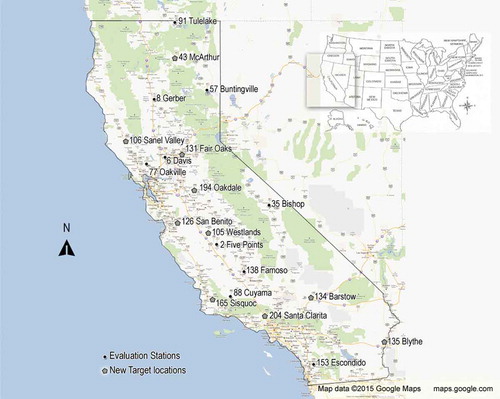
Fig. 2 The MASi index for solar radiation and temperature calculated using running averages of 1, 5, 10, 15, 20, 25 and 30 days.

Table 1 The CIMIS stations used in this study.

Station number	Name	Elevation (m)	Latitude (deg)	Longitude (deg)	Average annual
					Rs (mm d^-1)	RH (H)	T (ºC)	U (m s^-1)
Evaluation dataset
2	FivePoints	86.9	36.34	120.11	7.6	57.4	17	2.6
6	Davis	18.3	38.54	121.78	7.2	61.1	15.5	2.5
8	Gerber	76.2	40.05	122.16	7.1	62.7	16.2	2.6
35	Bishop	1271	37.36	118.4	8.2	38.7	12.8	1.6
57	Buntingville	1220.7	40.29	120.43	7.5	54.5	9.8	2.3
77	Oakville	57.9	38.43	122.41	6.9	71.4	14.3	1.7
88	Cuyama	698	34.93	119.61	7.7	54.4	14.2	2.2
91	Tulelake	1229.9	41.96	121.47	6.8	62.4	8.1	2.2
138	Famoso	126.5	35.6	119.21	7.2	59.7	16.7	1.5
153	Escondido SPV	118.9	33.08	116.98	7.4	62.9	16.0	1.8
New target locations
43	McArthur	1009	41.03	121.27	7.5	62.2	9.9	2.2
105	Westlands	58.2	36.63	120.38	7.8	58.0	17.1	2.4
106	Sanel Valley	160	38.59	123.05	7.3	69.3	13.2	1.8
126	San Benito	103.6	36.85	121.36	7.4	75.4	13.6	1.5
131	Fair Oaks	80.8	38.65	121.22	7.3	64.7	16.0	1.5
134	Barstow	621.8	34.53	116.59	9.0	41.9	18.9	2.8
135	Blythe NE	83.8	33.56	114.67	8.6	48.7	21.6	2.4
165	Sisquoc	163.4	34.84	120.21	7.2	74.4	13.2	1.8
194	Oakdale	50	37.43	120.51	7.6	68.6	15.3	2.4
204	Sta Clarita	430	34.25	118.31	8.0	48.2	18.2	2.4

The daily relative humidity data from the CIMIS stations were validated by a range test, ignoring values outside the 20–100% range (Meek and Hatfield 1994). Temperature data were also screened, using a similar range test. Solar radiation measurements were compared against computed shortwave radiation expected under clear sky conditions. Whenever an error was detected in a parameter, the dataset of the whole day was eliminated, since the resulting PM ETo calculations would be unreliable. Usually inconsistent data were observed prior to the outright failure of the sensor. All data from 10 days prior to 10 days after any sensor failure were also eliminated due to their influence on the moving averages.

Daily HS ETo estimates were calculated using equation (3), while the FAO PM ETo estimates calculated by CIMIS were used. The daily extraterrestrial radiation (R_a) used in the HS equation was calculated by:

(4)

where d_r is the inverse relative Earth–Sun distance, ω_s is the sunset hour angle, φ is the latitude of the location and δ is the solar declination, as further explained by Allen et al. (1998).

Evaluation of existing annual climate patterns

Given the natural daily variability in the data, running averages were used to temporally smooth out the daily series of weather data from the above-mentioned stations. Simple running average is the unweighted mean of n datum points obtained through:

(5)

where y₁, y₂, y₃, …, y_n are the daily data, and n is the number of days being considered for the running average. The mean is obtained using an equal number of data on either side of the date.

The optimum size for the moving average is the smallest number that can reasonably smooth out the natural scatter in the data. To establish this optimum size, a statistic was developed that sums the square of the difference between consecutive values of the parameter, (P_i – P_i−1). The square root of the average difference is then divided by the average value of the parameter, P. The statistic, called the ‘moving average scatter index’ (MASi) can be defined as:

(6)

where n is the number of data in the sample. This statistic is calculated for moving averages of increasing sizes, and the optimum size is obtained when no important improvements in the value of the statistic are obtained by increasing the size of the moving average.

MASi was calculated for solar radiation and temperature, using the original values and 5-, 10-, 15-, 20-, 25- and 30-day moving averages. The results for Davis are presented in Fig. 2 and show that the original values of solar radiation have a greater scatter index than the original values of temperature. It was observed that for solar radiation, MASi improved visibly up to 20 days, and no further improvements in the value of MASi were observed when the size of the moving average was increased. For temperature, MASi improved up to 25 days, and then no important improvement was observed beyond that value. Therefore, 25-day moving averages were used for this work.

Since the HS equation is based directly on temperature measurements and indirectly on R_s estimates, in this work, the annual dynamics of the T–R_s relationship in the region was studied by plotting their running daily averages against each other. The evolution of K_T calculated from measured R_s values was also studied, both on a daily basis and as a function of R_s. Finally, the daily evolution of the FAO PM/HS ETo ratio was studied in order to better understand the seasonal pattern of variation in the ETo estimates produced by these two methods.

Calibration of new locations

A set of 10 new stations was selected from the CIMIS network (Table 1), with diverse elevations and distance to coast (Fig. 1), to be representative of the different areas of the region. These stations were used as new target locations where reduced-set ETo estimates are needed and no previous data exist for calibration. For each location, daily ETo estimates based on the HS methodology were calculated for the 2-year period between 1 January 2010 and 31 December 2011. To evaluate the merit of using seasonal patterns in calibration of reduced-set ETo equations, the new target stations were calibrated using the proposed methodology based on average seasonal calibration patterns for the region.

The improvement obtained through calibration was then statistically evaluated. A distinction should be made between scatter and bias. Bias can be defined as systematic deviation in data. Thus, the HS equation presents bias when it systematically over- or underestimates ETo. There is scatter when daily values do not agree with the reference methodology, even if long-term or annual averages do. To evaluate the scatter of the values and the quality of the fit between the HS estimates and the reference methodology, the coefficient of determination of the best-fit regression line, r², was used, which is the ratio of the explained variance to total variance, and is expressed as:

(7)

where n is the number of observations, O_i is the observed value, usually PM or lysimeter data, E_i, is the value estimated by the HS equation and Ō is the average of observed values. The main objection to using the coefficient of determination is that it improves with the size of the sample. Therefore, the quality of the estimates and scatter were additionally evaluated by the root mean square error, RMSE:

(8)

The most widely used indicator for measuring bias, is the mean bias error, MBE, which is defined as:

(9)

RESULTS AND DISCUSSION

Evaluation of existing annual climate patterns

The original equation developed by Hargreaves and Samani produces ETo estimates based on direct measurements of temperature and indirect estimates of solar radiation. The annual pattern of behaviour of these parameters can be studied through a correlation using moving averages of these two parameters. Figure 3 presents 25-day moving average daily values of temperature and radiation of the 10 stations from 2000 to 2009 and shows the average temperature plotted as the dependent variable against solar radiation. The normal irrigation period is considered to be 1 May to 30 September and is indicated in Fig. 3 with grey symbols. The results indicate a non-univocal relationship between radiation and air temperature—a ‘warming’ period can be observed during which the temperature trails behind the increasing solar radiation, and then a ‘cooling’ period in which the temperature drops more slowly than the solar radiation. It can be observed that this annual R_s–T cycle is divided into an ascending wing representing the spring/summer months, and a descending wing corresponding to the cooling of air during autumn and winter. The distance between the two lines is due to the existing delay in the warming or cooling of the Earth and air masses as a result of the seasonal variation in the R_s.

Fig. 3 Annual evolution of T, as a function of R_s (mm d^-1). The data represent 25-day moving averages of 10-year datasets of the CIMIS validation stations. It can be observed that R_s peaks on 24 June, while T peaks on 18 July. The irrigation season in considered as the period between 1 May and 30 September.

The data also indicate that R_s peaks around 24 June, while average temperature continues to increase for another three weeks. Temperature peaks on 18 July and then follows the decreasing pattern of R_s, confirming the behaviour of average temperature as a function of R_s, albeit with a 25-day delay. Based on these data, the main irrigation season in the Mediterranean climate can be divided into three phases: increasing R_s and T; decreasing R_s with increasing T; and decreasing R_s and T.

The same seasonal pattern of R_s–T relationship was observed in each of the individual stations, despite the great differences in their elevation (18–1230 m a.s.l.), and annual temperatures. The peak of radiation for the 10-year period ranged between 17 June in Bishop and 25 June in Oakville, Cuyama, Tulelake and Gerber. The temperature peak also varied slightly between the stations, ranging between 12 July in Davis and 23 July in Escondido.

The size of the moving average might have an influence on the established dates for the peaks. To evaluate this influence, moving averages of different sizes (5, 10, 15, 20, 25 and 30 days) were calculated for daily values of single stations, and then averaged. The values of the 10 stations for each size of moving average are presented in Fig. 4.

Fig. 4 Annual relation between solar radiation (R_s), and temperature (T), obtained using moving averages of 5, 10, 15, 20, 25 and 30 days.

The results show that as the moving averages ‘round-off’ the daily variability, the resulting values for the individual days change slightly. Effectively, the maximum average value of R_s decreased from 11.7 to 11.5 when the size of the moving average changed from 5 to 30 days. The maximum value of T also decreased from 24.2 to 23.3ºC.

Regarding the dates for peak radiation and temperature, these also changed slightly with the increasing size of the moving average. There is no apparent direct relationship between the size of the moving average and the actual dates. The changes seem to be related to the natural tendencies in the values of R_s and T which are emphasized depending on the size of the moving average.

In the HS equation, solar radiation is estimated based on the ∆T function multiplied by the empirical K_T coefficient. The value of K_T is fixed for the whole year and is usually assumed to be 0.17. Alternatively, actual K_T values can be obtained from observed daily solar radiation using Hargreaves’s original equation (equation (2)). The new K_T values can then be used instead of the original 0.17 for calibrating the HS equation (Samani 2000, Jabloun and Sahli 2008).

To study the annual variability of K_T values, these were calculated using actual daily R_s values and plotted in Fig. 5(a) as a function of the Julian day. The results show that the value of K_T is not constant, and evolves according to a parabolic function throughout the year. It increases with R_s, peaks on 22 June, and then decreases gradually, reaching a value of less than 0.14 on 21 December. It is possible to fit a curve to its evolution with a value of r² = 0.72.

When the calculated daily K_T values are plotted against the average daily measured R_s values (Fig. 5(b)), the two ascending and descending wings seem to overlap, indicating that the value of K_T can be obtained from R_s values alone. Additionally, it is noted that there is a sudden drop in the K_T for R_s values below 4, which represent the short winter days.

Fig. 5 Average daily evolution of K_T calculated from equation (2) for 10 stations, presented as a function of (a) the day of year and (b) R_s.

The seasonal variability of these parameters and their interaction indicate that a single annual correlation between the PM and HS ETo might not be the best option, specially since PM takes into account four climate parameters, and HS is based only on T and an estimate of R_s. Thus, it is important to establish seasonal relations between R_s and ETo calculated by the PM and HS methodologies, and use moving averages to smooth out irregularities.

Figure 6 presents the values of ETo estimates by the two methods plotted against daily R_s values. The results indicate that for both methods, the relation between R_s and ETo is not univocal and two different vales of ETo can be expected from the same R_s value, depending on the time of the year. The previously mentioned temperature lag seems to affect the estimates of crop ETo, resulting in a ‘warming’ and a ‘cooling’ period in the year.

Fig. 6 Daily correlation between R_s and the ETo calculated by the FAO PM and HS methods. The shaded area indicates approximately the irrigation season.

Regarding the ETo estimates by the two methods, it can be observed that the HS method underestimates ETo in the low and mid-range R_s values. After 7 June, the temperature-based HS equation continues to calculate increasing ETo and starts to overestimate daily ETo values compared to the FAO PM methodology. This results in an overestimation of the ETo by the HS methodology between 7 June and 10 September, totaling 17 mm of water. Additionally, there is a 5-day delay between the peaks of the PM methodology and the HS equation, where the former peaks at around 2 July, while the latter peaks on 7 July. This delay is probably caused by the fact that the HS equation uses mainly temperature and, as observed above, there is a delay of almost three weeks between an inflection in the solar radiation intensity and a perceptible change in the measured temperature.

In the case of individual stations, the delay between the peaks of daily ETo values calculated by the two methodologies varied between 20 days in Gerber and 1 day in Davis, Escondido and Buntingville. The maximum overestimation of the ETo by the HS equation was observed in Oakville and Bishop, with an overestimation of 8% and 15%, respectively.

For agricultural purposes, it is more important to calibrate the HS equation for the main irrigation period, which, under the Mediterranean climate of California, covers the May–September period. The temporal evolution of the daily average values of FAO PM/HS ratio are presented in Fig. 7. The results reveal that the ratio decreases from the beginning of the irrigation season until 17 July, which corresponds approximately to the temperature peak (Fig. 3). After the temperature peak, the FAO PM/HS ratio increases steadily until the end of the irrigation season, reaching a maximum of almost 1.1 by mid-October. These results show that the HS equation tends to overestimate ETo during the peak temperatures of June–August and underestimate it at lower temperatures.

Fig. 7 Annual evolution of the FAO PM/HS ratio. Regression lines were adjusted to the warming and cooling wings of the irrigation season.

By comparing Figs 5 and 7, it is possible to evaluate the influence of calculated K_T on the ETo estimates obtained by the HS equation. It can be observed that the calculated K_T values have a great influence on the FAO PM/HS ratio outside the irrigation season. Effectively, the low values of calculated K_T in January/February and then in November/December mean that equation (2) overestimates the HS ETo value for these months, and thus the FAO PM/HS ratios will also be low. During the dry season, the variability in the FAO PM/HS ratio seems to be more independent of the calculated K_T values.

These results indicate that annual calibration of the HS evapotranspiration equation can be misleading, since clear seasonal variations can be observed in the calibration coefficients. When using a single annual calibration coefficient, periods of over and underestimation can cancel each other, leading to the false impression that no calibration is necessary. But when analysing daily values, the HS equation is seen to overestimate ETo during most of the irrigation season, specially during the whole of the critical July–August period.

Validation in new locations

In order to evaluate the merit of the proposed seasonal calibration using region-wide calibration coefficients, 10 new locations were selected from the CIMIS network. These locations represent new target areas where it is necessary to calculate HS ETo for irrigation purposes and it was assumed that no previous data exist for calibration. This study was carried out using daily ETo estimates of a 2-year period, from 1 January 2010 to 31 December 2011.

The quality of the ETo estimates from these stations without any calibration is summarized in Table 2. The results indicate that both the MBE and RMSE are smaller when data from the whole year are considered. When only irrigation season data are considered, the average MBE increases from 0.351 to 0.400 mm, and the RMSE increases from 0.804 to 0.871. The coefficient of determination decreases from 0.893 to 0.674, which indicates that the performance of the HS equation decreases during the irrigation season, compared to when data for the whole year are used. This can be related to the fact that ETo values are smaller during the winter months, and thus the same relative error translates into a smaller absolute error than during the irrigation season.

Table 2 Average values of FAO PM and HS ETo estimates and statistics from the 10 new target locations before calibration (MBE and RMSE in mm d^-1).

	Average ETo (mm d^-1)		All year			Irrigation season
	PM	HS	MBE	RMSE	r^2	MBE	RMSE	r^2
43 McArthur	3.42	3.48	0.06	0.56	0.94	0.02	0.67	0.79
105 Westlands	4.49	4.34	−0.15	0.77	0.93	−0.44	0.92	0.70
106 Sanel Valley	3.46	3.84	0.37	0.72	0.91	0.49	0.81	0.78
126 San Benito	3.14	3.46	0.30	0.51	0.93	0.26	0.49	0.82
131 Fair Oaks	3.45	3.80	0.35	0.66	0.93	0.43	0.77	0.77
134 Barstow	5.50	4.62	−0.88	1.49	0.81	−1.11	1.89	0.22
135 Blythe NE	5.50	5.11	−0.39	1.10	0.83	−0.32	1.15	0.35
165 Sisquoc	3.16	3.38	0.22	0.52	0.87	0.23	0.45	0.80
194 Oakdale	3.77	3.86	0.09	0.55	0.95	−0.11	0.58	0.79
204 Sta Clarita	4.83	4.14	−0.69	1.16	0.82	−0.59	0.99	0.72
Average	4.07	4.00	0.35	0.80	0.89	0.40	0.87	0.67

The ETo estimates using HS equation at the new stations were calibrated using seasonal calibration with region-wide calibration coefficients, as proposed in this work. In this method, the daily ratios of the HS and FAO PM ETo estimates at the existing stations (historic data from the 2000–2009 period), and presented in Fig. 7, were used to calibrate the new target stations for the 2010–2011 period. The daily HS ETo estimates for each of the target locations were corrected using the historic HS/FAO PM relation for the corresponding date.

The results of the calibration are presented in Table 3 and show that the calibration did not provide for any gains in precision of the ETo estimates when whole year values were considered. The absence of improvements in the whole year estimates was expected given the very irregular pattern of the HS/PM ratio outside the irrigation season (see Fig. 7). But when only the irrigation season is considered, it is possible to observe a significant improvement in both MBE, which decreased from 0.40 to 0.36 mm d^-1, and r², which increased from 0.67 to 0.87. The improvement in the bias is important, since it represents greater long-term adjustment between the two methods, and thus better ETo estimates for irrigation and water management purposes. The proposed calibration did not improve RMSE in any of the periods considered, which was expected since the use of historic averages does not improve daily scatter in the daily ETo estimates.

This improvement in the bias and r² values for the irrigation season is promising, and indicates that this method can be used to pre-calibrate the HS equation for new stations in large areas based on historic values from existing reference stations. This methodology, involving the use of moving averages to obtain seasonal patterns of HS/PM ratios can be applied to other regions, providing a simple tool for improving ETo estimates with the Hargreaves-Samani equation using only temperature measurements.

Table 3 Statistics from the 10 new target locations after daily calibration using historic region-wide HS/FAO ratios (MBE and RMSE in mm d^-1).

	Average ETo (mm d^-1)		All year			Irrigation season
	PM	HS	MBE	RMSE	r^2	MBE	RMSE	r^2
43 McArthur	3.42	3.65	0.06	0.61	0.93	0.06	0.71	0.92
105 Westlands	4.49	4.56	−0.16	0.84	0.92	−0.16	0.99	0.91
106 Sanel Valley	3.46	4.02	0.38	0.75	0.90	0.38	0.77	0.92
126 San Benito	3.14	3.60	0.32	0.56	0.91	0.32	0.51	0.91
131 Fair Oaks	3.45	3.98	0.36	0.67	0.93	0.36	0.73	0.92
134 Barstow	5.50	4.82	−0.89	1.52	0.80	−0.89	1.92	0.76
135 Blythe NE	5.50	5.34	−0.39	1.10	0.81	−0.39	1.20	0.79
165 Sisquoc	3.16	3.54	0.26	0.56	0.85	0.26	0.46	0.85
194 Oakdale	3.77	4.06	0.10	0.62	0.94	0.10	0.62	0.93
204 Sta Clarita	4.83	4.34	−0.65	1.13	0.81	−0.65	1.03	0.81
Average	4.07	4.19	0.36	0.84	0.88	0.36	0.89	0.87

CONCLUSIONS

The results indicate the existence of annual R_s–T cycles in which T trails behind radiation with a delay of some 25 days. This phenomenon is associated with the warming of the soil and air masses by increases in daily solar radiation, and these remain relatively warm for more than three weeks when solar radiation starts to decrease. As a result, maximum temperature is reached some three weeks after the peak in solar radiation. Based on these data, the main irrigation season in the Mediterranean climate (1 May–30 September) can be divided into three phases: increasing R_s and T; decreasing R_s with increasing T; and decreasing R_s and T. The annual cycle itself can be divided into an ascending or warming wing which lasts until 18 July and a descending or cooling wing which continues until the end of December. It is noted that the size of the moving average can influence the exact dates of the peaks, but does not affect the tendencies observed.

This seasonal pattern of climate parameters has significant implications for ETo calculations, specially in the case of equations using reduced-set weather parameters. Thus, the relation between ETo estimates obtained by different equations will necessarily reflect the seasonal pattern of the weather parameters used. When compared to FAO PM, the HS equation underestimates ETo in the low and mid-range R_s values, and then overestimates ETo between 7 June and 10 September. During this period, the average total overestimation by the HS equation is 17 mm. This overestimation is at least partly due to the fact that the temperature based HS equation continues to calculate high ETo values based on increasing temperatures, while the PM equation is beginning to factor in the decrease in R_s, and thus produces smaller ETo values.

The value of K_T coefficient can be calculated from observed solar radiation. During the rainy months, important patterns were observed in the value of calculated K_T, which were then mirrored in the FAO PM/HS ratio. This indicates that at least some of the variability in the FAO PM/HS ratio can be attributed to the fact that the HS equation uses a constant value for K_T, while the value of this parameter follows seasonal patterns. These findings indicate the need for further study of this variation and the importance of seasonal calibration when using this and other reduced-set ETo equations in any region.

The results from the 10 CIMIS stations indicate that the HS equation produces ETo estimates that are in agreement with those obtained by the FAO PM equation, although the quality of the estimates is lowest during the important irrigation season, and thus the use of single whole year calibration coefficients can be misleading.

A method is proposed to pre-calibrate ETo estimates at new stations with no previous weather records. The method consists in the use of seasonal region-wide HS/FAO PM ratios obtained from moving averages, as described above. This calibration produced better ETo estimates and an important improvement in the coefficient of determination and in the bias, when only the irrigation season was considered. As expected, it did not affect the scatter of the daily values, as measured by RMSE.

The results also indicate that for irrigation purposes, the use of seasonal calibration using historic values can greatly improve ETo estimates by the Hargreaves-Samani equation in terms of bias.

Disclosure statement

No potential conflict of interest was reported by the author(s).

Acknowledgements

The authors would like to thank the anonymous reviewers for their important contribution to this work.

Additional information

Funding

This work was funded by FCT grant PTDC/AAC-AMB/ 113639/ 2009: Evaluation of climate changes impacts on irrigated systems and definition of adaptation measures.

REFERENCES

- Allen, R.G., et al., 1998. Crop evapotranspiration: guidelines for computing crop requirements. Irrigation and Drainage Paper no. 56. Rome, Italy: FAO.
- Bautista, F., Bautista, D., and Delgado-Carranza, C., 2009. Calibration of the equations of Hargreaves and Thornthwaite to estimate the potential evapotranspiration in semi-arid and sub-humid tropical climates for regional applications. Atmósfera, 22 (4), 331–348.
- DehghaniSanij, H., Yamamoto, T., and Rasiah, V., 2004. Assessment of evapotranspiration estimation models for use in semi-arid environments. Agricultural Water Management, 64, 91–106.
- Di Stefano, C. and Ferro, V., 1997. Evaluation of evapotranspiration by Hargreaves formula and remotely sensed data in semi-arid Mediterranean areas. Journal Agricultural Engineering Research, 68, 189–199.
- Droogers, P. and Allen, R.G., 2002. Estimating reference evapotranspiration under inaccurate data conditions. Irrigation and Drainage Systems, 16 (1), 33–45.
- Echnig, S., 2002. Role of technology in irrigation and advisory services: the CIMIS experience. In: Irrigation advisory services and participatory extenstion in irrigation management, FAO workshop, 24 July 2002, Montreal.
- Gavilán, P., Estévez, J., and Berengena, J., 2008. Comparison of standardized reference evapotranspiration equations in Southern Spain. Journal of Irrigation and Drainage Engineering, 134 (1), 1–12. doi:10.1061/ASCE0733-9437
- Gavilán, P., et al., 2006. Regional calibration of Hargreaves equation for estimating reference ET is a semiarid environment. Agricultural Water Management, 81, 257–281.
- Gonzalez, A., Villazón, M.F., and Willems, P., 2009. Reference evapotranspiration with limited climatic data in the Bolivian Amazon. In: 1st international congress of hydroclimatology, August, Cochabamba, Bolivia. SENAMHI.
- Hargreaves, G.H., 1975. Moisture availability and crop production. Transactions of the ASAE, 18 (5), 980–984.
- Hargreaves, G.H., 1994. Simplified coefficients for estimating monthly solar radiation in North America and Europe. Logan: Departmental Paper, Department of Biological and Irrigation Engineering, Utah State University.
- Hargreaves, G.H. and Allen, R.G., 2003. History and evaluation of hargreaves evapotranspiration equation. Journal of Irrigation and Drainage Engineering, 129 (1), 53–63.
- Hargreaves, G.H. and Samani, Z.A., 1982. Estimating potential evapotranspiration. Journal of the Irrigation and Drainage Division, 108 (3), 225–230.
- Hargreaves, G.H. and Samani, Z.A., 1985. Reference crop evapotranspiration from temperature. Applied Engineering in Agriculture, 1 (2), 96–99.
- Henggeler, J.C., et al., 1996. Evaluation of various evapotranspiration equations for Texas and New Mexico. In: C.R. Camp, E.J. Sadler, and R.E. Yoder, eds. Proceedings of the international conference on evapotranspiration and irrigation scheduling. 3–6 November 1996, San Antonio, TX, 962–967. Irrigation Association-International Committee on Irrigation and Drainage.
- Jabloun, M. and Sahli, A., 2008. Ajustement de l’e´quation de Hargreaves-Samani aux conditions climatiques de 23 stations climatologiques Tunisiennes. Bulletin Technique no. 2. Laboratoire de Bioclimatologie, Institut National Agronomique de Tunisie, 21.
- Jensen, D.T., et al., 1997. Computation of ETo under non ideal conditions. Journal of Irrigation and Drainage Engineering, ASCE, 123 (5), 394–400.
- Lee, K.H., 2010. Relative comparison of the local recalibration of the temperature-based evapotranspiration equation for the Korea Península. Journal of Irrigation and Drainage Engineering, 136 (9), 585–594.
- López-Urrea, R., et al., 2006. Testing evapotranspiration equations using lysimeter observations in a semiarid climate. Agricultural Water Management, 85, 15–26.
- Martínez-Cob, A. and Tejero-Juste, M., 2004. A wind-based qualitative calibration of the Hargreaves ETo estimation equation in semiarid regions. Agricultural Water Management, 64, 251–264.
- Meek, D.W. and Hatfield, J.L., 1994. Data quality checking for single station meteorological databases. Agricultural and Forest Meteorology, 69, 85–109.
- Orang, M.N., Grismer, M.E., and Ashktorab, H., 1995. New equations estimate evapotranspiration in Delta. California Agriculture, 49 (3), 19–21. doi:10.3733/ca.v049n03p19May-June
- Samani, Z., 2000. Estimating solar radiation and evapotranspiration using minimum climatological data. Journal of Irrigation and Drainage Engineering, 126 (4), 265–267.
- Samani, Z.A. and Pessarakli, M., 1986. Estimating potential crop evapotranspiration with minimum data in Arizona. Transactions of the ASAE, 29, 522–524.
- Sentelhas, C., Gillespie, T.J., and Santos, E.A., 2010. Evaluation of FAO Penman–Monteith and alternative methods for estimating reference evapotranspiration with missing data in Southern Ontario, Canada. Agricultural Water Management, 97, 635–644.
- Sepaskhah, A.R. and Razzaghi, F., 2009. Evaluation of the adjusted Thornthwaite and Hargreaves-Samani methods for estimation of daily evapotranspiration in a semi-arid region of Iran. Archives of Agronomy and Soil Science, 55 (1), 51–66.
- Temesgen, B., et al., 2005. Comparison of some reference evapotranspiration equations for California. Journal of Irrigation and Drainage Engineering, 131 (1), 73–84.
- Vanderlinden, K., Giráldez, J.V., and Meirvenne, M.V., 2004. Assessing reference evapotranspiration by the hargreaves method in Southern Spain. Journal of Irrigation and Drainage Engineering, 130 (3), 184–191.