Intercomparison across scales between remotely-sensed land surface temperature and representative equilibrium temperature from a distributed energy water balance model

Abstract

Quantifying the reliability of distributed hydrological models is an important task in hydrology to understand their ability to estimate energy and water fluxes at the agricultural district scale as well the basin scale for water resources management in drought monitoring and flood forecasting. In this context, the paper presents an intercomparison of simulated representative equilibrium temperature (RET) derived from a distributed energy water balance model and remotely-sensed land surface temperature (LST) at spatial scales from the agricultural field to the river basin. The main objective of the study is to evaluate the use of LST retrieved from operational remote sensing data at different spatial and temporal resolutions for the internal validation of a distributed hydrological model to control its mass balance accuracy as a complementary method to traditional calibration with discharge measurements at control river cross-sections. Modelled and observed LST from different radiometric sensors located on the ground surface, on an aeroplane and a satellite are compared for a maize field in Landriano (Italy), the agricultural district of Barrax (Spain) and the Upper Po River basin (Italy). A good ability of the model in reproducing the observed LST values in terms of mean bias error, root mean square error, relative error and Nash-Sutcliffe index is shown.

Editor Z.W. Kundzewicz; Associate editor D. Gerten

Résumé

Quantifier la fiabilité des modèles hydrologiques distribués est une tâche importante en hydrologie pour comprendre leur capacité à estimer les flux d’énergie et d’eau, pour la gestion des ressources en eau pendant les périodes de sécheresse et pour la prévision des crues, tant à l’échelle de la parcelle agricole qu’à l’échelle du bassin versant. Dans ce contexte, cet article présente la comparaison, à différentes échelles spatiales allant de la parcelle au bassin versant, entre la température d’équilibre représentative (TER) simulée issue d’un modèle hydrologique distribué, et la température de surface du sol (TSS) issue de la télédétection. L’objectif principal de l’étude est d’évaluer l’utilisation de la TSS obtenue par des données de télédétection opérationnelles à différentes résolutions spatiales et temporelles, pour la validation interne d’un modèle hydrologique distribué, de manière à contrôler l’exactitude du bilan de masse comme méthode complémentaire au calage traditionnel sur les mesures de débit aux sections de contrôle du cours d’eau. Les TSS modélisées et observées à partir de différents capteurs radiométriques situés à la surface du sol, sur un avion et sur ​​un satellite ont été comparées pour un champ de maïs de Landriano (Italie), du district agricole de Barrax (Espagne) et pour le haut bassin du Pô (Italie). Nous avons mis en évidence une bonne capacité du modèle à reproduire les valeurs de TSS observées en termes d’erreur moyenne du bilan, d’erreur quadratique moyenne, d’erreur relative et d’indice de Nash-Sutcliffe.

Key words:

• energy water balance model
• remote sensing
• land surface temperature

Mots clefs:

• modèle de bilan d’eau et d’énergie
• télédétection
• température de surface du sol

1 INTRODUCTION

Distributed hydrological models allow estimation of energy and water fluxes at various scales (local, basin, global) for water resources management, agriculture and flood forecasting purposes and are now a valid tool for engineering and agricultural practice, filling the gap in research investigation (Noilhan and Planton 1989, Famiglietti and Wood 1994, Bastiaanssen et al. 1998, Montaldo and Albertson 2001, Su 2002, Caparrini et al. 2004, Corbari et al. 2011). However, how to define the reliability of the implemented algorithms and their numerical validation is still an open problem due to the difficulties mainly related to the definition of variables that are representative of each single process and whether the measurements themselves are reliable (Beven and Binley 1992, Refsgaard and Knudsen 1996, Refsgaard 1997, Ciarapica and Todini 2002, Brath et al. 2004, Lohmann et al. 2004, Rabuffetti et al. 2008). Calibration and validation of distributed models at the basin scale generally refer to external variables, which are integrated catchment model outputs, and usually depend on comparison of simulated and observed discharges at available river cross-sections, which are usually very few. However, distributed models allow an internal validation due to their intrinsic structure (Dooge 1986, Fawcett et al. 1995), and so the model internal processes and variables can be controlled in each cell of the domain, e.g. soil moisture (SM), land surface temperature (LST) and evapotranspiration fluxes (ET). Hence, there is the opportunity to increase the flux control points so that mass balance accuracy can be improved. At the local scale, evapotranspiration is easily measurable with eddy covariance stations and it can be used for internal control of distributed models (Wilson et al. 2002), whereas, at basin or global scales, the monitoring of energy fluxes or soil moisture is more complicated due to the lower footprint representativeness of ground data (Ferguson et al. 2010).

Satellite data, which are intrinsically spatial in nature, can be used for the internal calibration/validation of distributed hydrological models if they are based on energy and water balance equations. Satellite images are important tools for use in conjunction with distributed models, although their reliability should be analysed. In recent years, a large number of satellites have been launched for the direct retrieval of soil moisture from passive to active microwave sensors such as AMSR-E, ASCAT or SMOS (Kerr et al. 2001, Naeimi et al. 2009, Wagner et al. 2008). However, some problems remain if these images are to be used in conjunction with hydrological models for operational water management applications. One of the main aspects is linked to the spatial resolution of the available products, which ranges between 25 and 50 km and is too coarse for model output comparison.

Land surface temperature (LST) satellite information seems to solve many limitations and difficulties of the technology based on microwave satellite images, although some uncertainties should be addressed, particularly over heterogeneous areas: their spatial resolution, scan angle of view of the sensor and surface emissivity (Sobrino et al. 1994, Jacob et al. 2004, Kustas et al. 2004, Sòria and Sobrino 2007). Recently some satellites have been launched with on-board sensors in the thermal infrared range, such as AATSR, MODIS and SEVIRI, with a low spatial resolution (1–5 km) but high temporal resolution (15 min to 12 h).

The LST is a critical model state variable and remotely-sensed LST can be effectively used, in combination with energy and mass balance modelling, to monitor latent and sensible heat fluxes. Indeed, through this system of equations, a link between LST, SM and latent and sensible heat fluxes is generated. The research community has widely used LST images from different sensors as input to energy and water balance models for evapotranspiration estimates (Kalma et al. 2008). Two main types of energy water balance models have been set-up: (a) models that compute evapotranspiration as the residual term of the energy balance equation using LST as input data, e.g. the SEBAL (Bastiaanssen et al. 1998), SEBS (Su 2002), TSEB (Norman et al. 1995) and S-SEBI (Roerink et al. 2000), and (b) models that solve the water and energy balances for LST, e.g. VIC (Liang et al. 1994) and TOPLATS (Famiglietti and Wood 1994). However, little effort has been made to understand whether LST detected by remote sensing can be a representative proxy of water balance processes at the surface, such that LST can be used to calibrate and validate hydrological models.

Given this context, the purpose of this work is to evaluate the use of LST retrieved from remote sensing data at different spatial and temporal resolutions for the internal validation of a distributed hydrological model to control its mass balance accuracy as a complementary method to traditional calibration/validation with streamflow measurements. To achieve this objective, an intercomparison across scales between modelled and observed land surface temperatures is performed to understand if these two are comparable. The analysis at the local scale is a support for the analyses at bigger scales so as to understand the individual hydrological processes and the behaviour of LST in different conditions, such as during night-time and daytime, or over bare soil or vegetation. These analyses are a first step towards the possible use of LST for the calibration of hydrological model parameters (soil and vegetation parameters) or for data assimilation.

The proposed approach contributes to the research direction highlighted 30 years ago by Jim Dooge (Dooge 1986), who encouraged the scientific modelling community to analyse the behaviour of the model internal state variables (e.g. soil moisture and its proxy) in addition to the traditional external fluxes (e.g. discharge) to obtain better understanding of hydrological processes and model analysis.

The distributed hydrological model, Flash-flood Event-based Spatially-distributed rainfall–runoff Transformation – Energy Water Balance model (FEST-EWB) (Mancini 1990, Corbari et al. 2011), is used. Several case studies have been carried out on areas ranging from agricultural district areas to river basins using data from operational satellite sensors and specific airborne flights. The case studies include a maize field in Landriano (Italy), the agricultural district of Barrax (Spain) and the Upper Po River basin (Italy).

2 THE ENERGY WATER BALANCE ALGORITHM IN THE FEST-EWB MODEL

The FEST-EWB model is a distributed hydrological energy water balance model that computes all the main processes of the hydrological cycle in each cell of the domain and runs in continuous time. Detailed descriptions and updates of FEST-EWB are available: Mancini (1990), Rabuffetti et al. (2008), Corbari et al. (2009, 2010, 2011) and Ravazzani et al. (2011).

Inputs to the model are: meteorological data (i.e. air temperature, incoming shortwave radiation, wind velocity, precipitation, air humidity), distributed maps of soil parameters (i.e. the digital elevation model, saturated hydraulic conductivity, field capacity, wilting point and soil depth) and vegetation parameters (i.e. leaf area index and vegetation height).

The energy budget of the soil–vegetation–low atmosphere system is solved by looking for the representative equilibrium temperature (RET), defined as the land surface temperature that closes the energy balance equation for any pixel of the basin surface. The model solves the system between energy and mass balances at the ground surface:

where SM (-) is the volumetric soil water content of the layer, P (mm s^-1) is the precipitation rate, R (mm s^-1) is the runoff flux, PE (mm s^-1) is the drainage flux, ET (mm s^-1) is evapotranspiration, d_z (mm s^-1) is the soil depth, R_n (W m^-2) is the net radiation, G (W m^-2) is the soil heat flux, H (W m^-2) is the sensible heat flux, LE (W m^-2) is the latent heat flux and dS/dt encloses the energy storage terms, such as the photosynthesis flux and the crop and air enthalpy changes.

These equations are solved explicitly with respect to RET, which includes the thermodynamic heterogeneity of the pixel surface and the link with the aerodynamic resistance in the turbulent fluxes estimate. In theory, the computed RET should thus be congruent with radiometric measurements from remote sensing (Norman and Becker 1995), so allowing comparison between them. In particular, ET is linked to the latent heat flux through the latent heat of vaporization (λ) and the water density (ρ_w):

(3)

The latent heat flux is then computed as:

(4)

where ρ_a is the air density, γ is the psychrometric constant (Pa °C^-1), f_v is the vegetation fraction and c_p is specific heat of humid air (MJ kg^-1 K^-1). The saturation vapour pressure (e*) is computed as function of the RET (Brutsaert 2005) and the vapour pressure (e_a) as a function of air temperature. The canopy resistance (r_c) is expressed following Jarvis (1976), while the soil resistance (r_s) according to Sun 1982. The aerodynamic resistance (r_a for vegetation and r_abs for bare soil) is computed using the Thom model (Thom 1975).

3 STUDY SITES

Model validation at the local/field scale is performed for a maize field in Landriano (Italy), the agricultural district is in the Barrax area in Spain, while for basin-scale analysis, the Upper Po River basin (Italy) is considered (Fig. 1).

Fig. 1 The validation sites: Landriano (Italy; 0.01 km²) and Barrax (Spain; 12 km²) (from Google Images) and the Upper Po River basin (Italy; about 38 000 km²) from a MODIS RGB image.

3.1 Field scale

Landriano eddy covariance station (45.19N, 9.15E) is located on the Po River plain (Italy) and operated by the Politecnico of Milano and University of Milano. The site is an experimental field of maize of 0.01 km² surrounded by other maize fields. The data used in this work were measured from 13 March to 11 October 2006. Maize was planted on 1 June and harvested on 11 October at a height of 224 cm. The station is equipped with different sensors to measure the principal mass and energy fluxes, such as net radiation, evapotranspiration and soil moisture at different depths (Corbari et al. 2012). In particular, ground land-surface temperature, used for model validation, was measured by the CNR1 with a Kipp and Zonen radiometer located at 5 m height. Data were stored every 30 minutes. Land surface temperature was also retrieved from MODIS on board the operational satellites Terra and Aqua, at a spatial resolution of 1 km in the thermal infrared bands (Barnes et al. 1998). This comparison was made at 1-km spatial resolution because the maize field is quite homogeneous and is surrounded by other maize fields.

A total of 104 daily and nocturnal images of MODIS11 LST products (MYD11A1 and MOD11A1 (https://lpdaac.usgs.gov/)) were selected for the whole simulation period. The dataset of modelled RET was created using only the values simulated during the MODIS satellite overpass. A similar dataset was obtained for observed LST from the ground radiometer located in the field.

Soil moisture was measured by CS616 Campbell Scientific probes at different depths, from 10 cm to 65 cm. The FEST-EWB model was run at a temporal resolution of 30 min and at point scale. The soil depth was set equal to 60 cm, which corresponds to the maximum measured root length.

3.2 Agricultural district

The agricultural district of Barrax (39.3N, 2.6W), near Albacete in Spain, is an extremely heterogeneous area characterized by a patchwork of irrigated and non-irrigated fields of different shapes and sizes that are cultivated with winter cereals, corn, barley/sunflower, onions and other vegetables, or are fallow. The weather is very dry and hot during summer. This area was selected as a test site for a field campaign during June–July 2005 in the framework of the international SENtinel-2 and FLuorescence EXperiment (SEN2FLEX) project funded by the European Space Agency (University of Valencia 2005; www.uv.es/leo/sen2flex/). During the field campaign, 12 daytime and night-time overpasses were performed by an aeroplane with the Airborne Hyperspectral Scanner (AHS) on board. Land surface temperature images were obtained at a spatial resolution of 10 m with the Temperature and Emissivity Separation (TES) method (Gillespie et al. 1998), as reported in detail in Sobrino et al. (2008). FEST-EWB was run at a spatial resolution of 10 m and a temporal resolution of 10 min due to computing limitations.

The AHS images were then resampled to the 10 m spatial resolution of FEST-EWB so as to be directly comparable.

3.3 Basin scale

The test area is the Upper Po River basin above the confluence of the Po and Ticino rivers at the Ponte della Becca cross-section in northern Italy, with a total area of about 38 000 km². This basin drains an alpine region with mountains covering 37% of its territory, and includes 2300 km² of rice paddies (6% of total area) in the flat plain, which are completely submerged by irrigation between May and October.

Meteorological data for 1 January 2000 to 31 December 2003 at an hourly or sub-hourly time step, were collected by the monitoring systems of Arpa Piemonte, Lombardia and Valle d’Aosta and of Switzerland (Rabuffetti et al. 2008). In total, 455 air temperature stations are available, 169 record relative air humidity and 80 record incident short-wave solar radiation. Observed ground data were interpolated every hour to a regular grid using the inverse distance weighting method. For air temperature interpolation, a correction that takes into account the reduction of temperature with altitude with a constant lapse rate of –0.0065°C m^-1 was used, while, for the incoming shortwave radiation, the effect of complex topography was taken into account (Corbari et al. 2011).

Satellite images of land surface temperature are acquired from MODIS sensor (MYD11A1 and MOD11A1) products. For the four years of simulation, 2000–2003, 130 daytime and night-time images having cloud cover <20% over the entire area were selected,.

FEST-EWB was run at the satellite data spatial resolution of 1 km and with a temporal resolution of 1 hour.

4 COMPARISON BETWEEN REMOTE SENSING LST AND MODELLED RET

The FEST-EWB model is now validated at different spatial and temporal scales by comparing simulated RET and observed LST recorded at different spatial resolutions by radiometric sensors located on the ground surface, on the aeroplane and on satellites.

4.1 Statistical parameters

For the evaluation of RET estimates, the mean bias error (MBE), the root mean square error (RMSE) and the relative error (RE) are computed as follows:

(5)

(6)

(7)

where RET_i is the ith representative equilibrium temperature simulated by FEST-EWB, LST_i is the ith land surface temperature measured by a radiometer, n is the sample size, and LST is the average of measured land surface temperature.

Moreover the Nash-Sutcliffe efficiency index, η, is also computed (Nash and Sutcliffe 1970):

(8)

The Nash-Sutcliffe efficiency is commonly used to assess the predictive power of hydrological models. It can range from −∞ to 1. Essentially, the closer the model efficiency is to 1, the more accurate the model is.

4.2 Field scale

In Fig. 2, RET from FEST-EWB and measured LST from ground and satellite radiometers are compared and the results are reported in a scatter plot. A linear regression forced through the origin between RET (x) and LST from the station (y) is computed giving y = 0.97x (R² = 0.91), while an angular coefficient of 0.90 is obtained (R² = 0.90) when modelled values (x) are compared with the satellite ones (y).

Fig. 2 Field-scale comparison between simulated RET and LST (°C) measured at the station and retrieved from MODIS. The regression equation and R² are reported.

The evaluation parameters are summarized in Table 1. The Nash and Sutcliffe index reaches high values both for the comparison between RET and LST from the station, where η is equal to 0.91, and for the comparison between RET and LST from MODIS (η = 0.85). Low values of MBE, RE and RMSE are obtained for both the satellite and ground data, confirming the good capability of the model in reproducing observed land surface temperatures.

Table 1 Field-scale statistical parameters between RET (°C) and LST (°C) from the ground radiometer and from MODIS (Std Dev: standard deviation).

Radiometer		MBE (Std Dev) (°C)	RMSE (°C)	RE (%)	η
MODIS	Total data	2.2 (2.1)	2.5	8.1	0.85
	Diurnal data	2.4 (2.1)	3.3	11.0	0.79
	Nocturnal data	–0.66 (3.3)	2.1	11.6	0.83
	Bare soil period	2.9 (2.4)	5.3	10.5	0.79
	Vegetation period	1.8 (1.6)	2.4	7.4	0.86
Station	Total data	0.6 (1.6)	1.6	2.2	0.91
	Diurnal data	1.5 (1.6)	2.2	3.4	0.85
	Nocturnal data	–1.4 (2.0)	2.6	–1.8	0.9
	Bare soil period	–0.3 (2.1)	2.1	–2.9	0.87
	Vegetation period	0.2 (1.7)	2.4	0.6	0.92

The statistical parameters were then analysed in more detail differentiating between daytime and night-time data, and between vegetation and bare soil periods. During daytime, the observed ground and satellite data are always higher than modelled RET, whereas the opposite occurs at night. From the comparison with ground measured LST, no relevant difference is found between the bare soil period and the vegetated one, for both errors are similar, with MBE between –0.3 and 0.2°C and RMSE between 2.1 and 2.4°C (Table 1). However, when RET is compared to MODIS, higher errors are found when the field is without vegetation. This is probably linked to the spatial resolution of the satellite images which cover a bigger area than the analysed field. The Landriano field is bordered by a few trees which may influence the land MODIS surface temperature.

As previously stated, land surface temperature can be used as a control of soil moisture dynamics as represented in the FEST-EWB model through the system of mass and energy balance equations which are linked by evapotranspiration. Figure 3 compares the observed soil moisture, defined as the average over the vertical between the measurements at 10, 20, 35 and 65 cm, and the modelled SM; the reported data, from day 195 to day 266, show a good accordance during dry as well as wet periods. In fact, MBE is equal to 0.007, RMSE to 0.03, RE to 6% and η is equal to 0.81.

Fig. 3 Field-scale comparison between simulated and observed SM (-) from 14 July to 2 October 2006.

4.3 Agricultural district

The RET values from FEST-EWB were compared with LST retrieved from AHS images during the 12 flights. In Fig. 4, RET and LST from AHS, resampled to 10 m are reported for 13 July at 13:45 UTC+1, as an example. Histograms of LST from AHS and of the RET show similar frequency distributions. These are characterized by a bimodal distribution due to the distinction between crops and bare soil; although at lower temperatures more classes are identified due to the presence in the fields of crops at different growth stages and of different soil moisture conditions. The map of RET minus LST from AHS shows low values in all pixels (Fig. 4) indicating that the model is able to correctly reproduce the higher values of LST as well as the cooler pixels. Model ability to reproduce observed LST is also confirmed by the spatial autocorrelation functions (AC) of these two variables (Fig. 5) under the hypothesis of a stochastic process and of isotropy; thus AC is a function only of the distance between two points and not of the direction. The autocorrelation function of the simulated variable behaves in the same way as the observed LST AC function, confirming the success of the model in reproducing observed heterogeneity.

Fig. 4 Agricultural district-scale values of RET (°C) and LST (°C) from AHS and their difference (RST – LST; °C), and SM (-) from FEST-EWB for 13 July 2005 at 13:45: maps and histograms.

Fig. 5 Agricultural district-scale spatial autocorrelation functions (AC) for RET (°C) and LST (°C) from AHS and SM (-) from FEST-EWB for 13 July 2005 at 13:45.

Furthermore, in Fig. 4, a simulated soil moisture map and its histogram are reported for 13 July showing, from a first simple look, the link between land surface temperature and soil moisture. In fact the hotter pixels are associated with drier pixels, while the cooler ones are the wetter. This spatial agreement is confirmed by the AC function of soil moisture which looks quite similar to the AC of RET and of LST from AHS (Fig. 5).

The FEST-EWB evaluation parameters were then computed for 12 dates: MBE (difference between RET and LST from AHS), RMSE, RE and η are plotted in Fig. 6. MBE ranges between 0.88 and –1.24°C, RMSE between 1.31 and 3.3°C, while RE and η are between 1.83 and –5.69% and 0.62 and 0.85 respectively. These statistical results endorse the success of the model in correctly reproducing high-resolution land surface temperature values linked to vegetation type, growth vegetation period and irrigation.

Fig. 6 Agricultural district-scale statistics for comparison between RET (°C) and LST (°C) from AHS for the 12 available images: (a) MBE, (b) RMSE, (c) RE and (d) η.

In Table 2 the mean evaluation parameters are reported for all the images. Moreover daytime and night-time values are highlighted showing better agreement between FEST-EWB RET and LST from AHS during day than night.

Table 2 Agricultural district-scale statistical parameters between RET (°C) and LST (°C) from AHS for the 12 available images. MBE and Std Dev (°C), RMSE (°C), RE (%) and η are computed considering the total database, diurnal and nocturnal data, bare soil and vegetated fields.

	MBE (Std Dev) (°C)	RMSE (°C)	RE (%)	η
Total data	–0.33 (2.5)	2.5	–1.4	0.78
Diurnal data	–0.15 (2.5)	2.4	–0.6	0.81
Nocturnal data	–1.21 (1.3)	2.9	–3.6	0.62
Bare soil	–0.2 (1.5)	1.3	–1.1	0.91
Vegetation with fractional cover >0.8	0.1 (2.1)	2.2	–2.1	0.77
Sparse vegetation	–0.5 (2.9)	3.1	–3.5	0.64

The statistical parameters were also computed to distinguish between bare soil, vegetation with fractional cover >0.8 and sparse vegetation. In Table 2, an RMSE of 1.3°C is found for bare soil, of 2.2°C for dense vegetation, while a higher value, 3.1°C, is found for sparse vegetation fields. This result is linked to the difficulty of correctly defining the roughness of a complex scattered area in the hydrological model and also the emissivity in LST retrieval in airborne images (Sobrino et al. 2008).

4.4 Basin scale

At the basin scale, land surface temperature data retrieved from satellite images are robust for the validation of distributed hydrological models, providing many control points and so complementing traditional calibrations with discharge measurements at a few available control cross-sections.

In Fig. 7, as an example, 16 maps of LST from MODIS and RET are reported for 2003 and illustrate the good ability of the model in reproducing satellite data for summer as well as winter periods. Moreover, the different thermodynamic behaviour of the mountains, with lower temperature, and the plains, with higher temperature, is clearly visible in the observed maps as well as the simulated ones. This similarity is also confirmed by the frequency distribution analyses reported in Fig. 8 for three selected dates, 25 January at 13:00, 16 March at 13:00 and 7 June at 15:00 for the year 2003. A similar distribution of pixels number is found between RET and MODIS LST in each class. The analysis of histograms has been performed for the entire database, but is not reported here.

Fig. 7 Basin-scale images comparing RET (°C) and LST (°C) from MODIS for selected images for 2003.

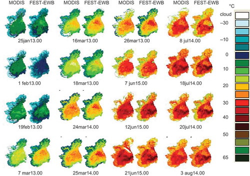
Fig. 8 Basin-scale histograms comparing RET (°C) and LST (°C) from MODIS for 25 January at 13:00, 16 March at 13:00 and 7 June at 15:00, in 2003.

Autocorrelation functions of LST from MODIS and RET have been computed to understand the capability of FEST-EWB to correctly reproduce the surface heterogeneity of the Upper Po River basin. Autocorrelation functions for the same dates as used to compute histograms (25 January at 13:00, 16 March at 13:00 and 7 June at 15:00 for 2003) show similar behaviour of LST from MODIS and RET from FEST-EWB with a similar degree of correlation decreasing with the distance (Fig. 9).

Fig. 9 Basin-scale autocorrelation functions (AC) for RET (°C) and LST (°C) from MODIS, and SM (-) from FEST-EWB for 25 January at 13:00, 16 March at 13:00 and 7 June at 15:00, in 2003.

The evaluation parameters are also estimated at the catchment scale: MBE, RSME, RE and η are reported in Fig. 10 for each of the 130 images. MBE lies between –3.6 and 4.3°C, RMSE is between 2.2 and 6.3°C, RE ranges from 2.6 to 6.5%, while η is between 0.4 and 0.8. Furthermore, modelled RET over the four years of simulation is, on average, 2.9°C higher than satellite LST with a standard deviation of 5.8°C and a Nash-Sutcliffe index η of 0.8 (Table 3). These results indicate that the model is in reasonable agreement with observed land surface temperatures.

Fig. 10 Basin-scale statistical parameters for comparison between RET (°C) and LST (°C) from MODIS for the 130 selected images: (a) MBE, (b) RMSE, (c) RE and (d) η.

Table 3 Basin-scale statistical parameters between RET (°C) and LST (°C) from MODIS for the 130 selected images. MBE and Std Dev (°C), RMSE (°C), RE (%) and η are computed considering the total database, diurnal and nocturnal data, and according to vegetation types coverage.

	MBE (Std Dev) (°C)	RMSE (°C)	RE %	η
Total basin	2.9 (5.8)	5	5.1	0.8
Diurnal data	1.49 (4.5)	4.7	3.5	0.78
Nocturnal data	–1.45 (3.1)	3.8	1.0	0.82
Forest	2.1 (6.4)	6.4	4.5	0.79
Agricultural area	3.4 (5.7)	5.1	6.8	0.73
Pasture and brushwood area	2.2 (4.9)	4	4.8	0.75
Rice paddies	2.2 (5.7)	4.7	3.7	0.83
Water	1.9 (2.9)	4.3	2.5	0.88

Due to the very high heterogeneity of the basin, a more detailed analysis is needed to understand the thermodynamic behaviours of the different types of soil–vegetation system. So the basin was subdivided into more homogeneous areas using CORINE land cover maps (CEC 1994, EEA 2000) updated in 2000 for the Italian part and in 1990 for the Swiss part. Five homogeneous types of land cover were identified: forest, agricultural area, pasture and brushwood area, water and rice paddies. Urban areas were excluded because the model does not simulate them. Table 3 shows MBE, RSME, RE and η computed for these land cover types and shows that good accuracy is reached for forest, rice paddies and water surface (low values of MBE, RSME, RE) because the vegetation parameters can be identified reasonably. The agricultural plain area shows bigger errors, a mean difference of 3.4°C and standard deviation of 5.7°C, due to the difficulty of exactly representing the vegetation dynamics in these large areas, such as the type of crop and its exact sowing and harvesting dates, and knowing the irrigation dates for each field.

Soil moisture maps and their autocorrelation functions from FEST-EWB were also considered due to the possible influence of land surface temperature on water balance dynamic. Figure 9 also shows AC functions of SM for the three dates and a good agreement between modelled and observed land surface temperature is evident.

5 DISCUSSION

An intercomparison across scales between remotely sensed LST and RET from FEST-EWB has been presented and similar results have been found. Lower errors are obtained at the local/field scale, where processes and parameters are easily controllable, than at the basin scale where more assumptions about the individual processes are necessary and there are greater uncertainties related to the heterogeneity of a single pixel for the definition of soil and vegetation parameters.

Furthermore, at all scales during daytime, observed ground and satellite LST are always slightly higher than modelled RET, while the opposite is valid during the night. At local scale no relevant differences are found in terms of statistical errors between the bare soil and the vegetation period; in contrast, for the Barrax area the fields with sparse vegetation are characterized by the highest errors, probably due to the difficulty of correctly defining the aerodynamic roughness over the complex scattered area. For the Upper Po River basin, greater errors are highlighted over non-natural vegetated areas due to the difficulties of exactly representing the vegetation dynamics linked to sowing and harvesting and the exact type of crop, and also to the irrigation dates for each single field.

These statistical results of the comparison between observed LST and simulated RET at different scales should be seen in terms of hydrological applications with the scope of estimating evapotranspiration fluxes, soil water content and river discharge, and not as the calibration of remote sensing algorithms. The importance of performing analyses at the local scale, where all the main processes are monitored, is highlighted throughout the paper. In fact, point studies are a help in understanding the hydrological processes, such as the different behaviour of land surface temperature during night-time and daytime, or over bare soil or vegetation, and in implementing the hydrological model at basin scales.

Furthermore, remote sensing imagery uncertainty, linked to the retrieval algorithms, should also be taken into account. In fact the definition of satellite LST over heterogeneous areas should be analysed regarding their spatial resolution, the scan angle of view of the sensor and emissivity (Sobrino et al. 1994, Jacob et al. 2004). Sobrino et al. (2003) analysed the accuracy of the MODIS LST product showing that the mean bias with ground data is equal to 2 K, which is comparable to the modelled RET errors.

6 CONCLUSIONS

In this paper, an intercomparison across scales between remotely sensed LST and representative equilibrium temperature from a distributed energy water balance model has been presented, showing the feasibility of using land surface temperature retrieved from remote sensing data at different spatial and temporal resolutions as a control of mass balance accuracy in a distributed hydrological model of each pixel of the domain, due to the effect of LST on energy and mass flux estimates. The results of the comparison between RET from FEST-EWB and remotely-sensed LST data at different spatial scales presented in this work indicate that the modelled RET is in reasonable agreement with LST measured from remote sensing in a hydrological context for operational applications in water management. The analyses performed at different spatial scales provide insight to the behaviour of individual processes at the local scale to successively apply the procedures at larger scales.

Simulated RET was compared to observed ground and satellite LST for the Landriano maize field and good values of the evaluation parameters were found: MBE 2.2 and 0.6°C, RE 8.1 and 3.2%, RMSE 0.85 and 0.91, η 0.85 and 0.91, respectively for MODIS images and ground data. In the Barrax agricultural area, modelled RET were found to be in reasonable agreement with observed LST data at higher spatial resolution: MBE –0.33°C, RE –1.4%, RMSE of 2.46°C and η 0.78. The comparison between RET and LST from MODIS performed for the different types of land cover in the Upper Po River basin showed the good ability of the model in reproducing the observed values in terms of MBE (2.9°C), RMSE (5.1°C), RE (5 %) and η (0.8).

This intercomparison showed that modelled RET from a distributed energy water balance model can be comparable to remotely sensed LST at different spatial scales, and so LST from remote sensing can now be used in FEST-EWB for data assimilation or for model parameter calibration.

Funding

This work has been developed in the framework of the ACQWA EU/FP7 project (grant no. 212250) “Assessing Climate impacts on the Quantity and quality of WAter”, of the Azioni Integrate Italia–Spagna (2009–2010) project (IT09G9BLE4) “Land surface temperature from remote sensing for operative validation of an hydrologic energy water balance model”, supported by the Italian Ministry of University and Scientific Research in collaboration with Prof. J.A. Sobrino of the Global Change Unit (Universitat de Valencia) and the ACCA project funded by Regione Lombardia “Misura e modellazione matematica dei flussi di ACqua e CArbonio negli agro-ecosistemi a mais”.

REFERENCES

- Barnes, W.L., Pagano, T.S., and Salomonson, V.V., 1998. Prelaunch characteristics of the moderate resolution imaging spectroradiometer (MODIS) on EOS-AM1. IEEE Transactions on Geoscience and Remote Sensing, 36 (4), 1088–1100. doi:10.1109/36.700993
- Bastiaanssen, W.G.M., et al., 1998. A remote sensing surface energy balance algorithm for land (SEBAL) 1. Formulation. Journal of Hydrology, 212–213, 198–212. doi:10.1016/S0022-1694(98)00253-4
- Beven, K. and Binley, A., 1992. The future of distributed models: model calibration and uncertainty prediction. Hydrological Processes, 6, 279–298. doi:10.1002/hyp.3360060305
- Brath, A., Montanari, A., and Toth, E., 2004. Analysis of the effects of different scenarios of historical data availability on the calibration of a spatially-distributed hydrological model. Journal of Hydrology, 291 (3–4), 232–253. doi:10.1016/j.jhydrol.2003.12.044
- Brutsaert, W., 2005. Hydrology: an introduction. Cambridge: Cambridge University Press.
- Caparrini, F., Castelli, F., and Entekhabi, D., 2004. Estimation of surface turbulent fluxes through assimilation of radiometric surface temperature sequences. Journal of Hydrometeorology, 5, 145–159. doi:10.1175/1525-7541(2004)005<0145:EOSTFT>2.0.CO;2
- CEC (Commission of the European Communities), 1994. CORINE land cover Technical guide. Luxembourg: Commission of the European Communities.
- Ciarapica, L. and Todini, E., 2002. TOPKAPI: a model for the representation of the rainfall-runoff process at different scales. Hydrological Processes, 16, 207–229. doi:10.1002/hyp.342
- Corbari, C., et al., 2009. Elevation based correction of snow coverage retrieved from satellite images to improve model calibration. Hydrology and Earth System Sciences, 13, 639–649. doi:10.5194/hess-13-639-2009
- Corbari, C., et al., 2010. Land surface temperature representativeness in a heterogeneous area through a distributed energy-water balance model and remote sensing data. Hydrology and Earth System Sciences, 14, 2141–2151. doi:10.5194/hess-14-2141-2010
- Corbari, C., Masseroni, D., and Mancini, M., 2012. Effetto delle correzioni dei dati misurati da stazioni eddy covariance sulla stima dei flussi evapotraspirativi. Italian Journal of Agrometeorology, 1, 35–51.
- Corbari, C., Ravazzani, G., and Mancini, M., 2011. A distributed thermodynamic model for energy and mass balance computation: FEST-EWB. Hydrological Processes, 25, 1443–1452. doi:10.1002/hyp.7910
- Dooge, J.C.I., 1986. Looking for hydrologic laws. Water Resources Research, 22 (9S), 46S–58S. doi:10.1029/WR022i09Sp0046S
- EEA, 2000. CORINE land cover technical guide – Addendum 2000. Copenhagen: EEA.
- Famiglietti, J.S. and Wood, E.F., 1994. Multiscale modeling of spatially variable water and energy balance processes. Water Resources Research, 30, 3061–3078. doi:10.1029/94WR01498
- Fawcett, K.R., et al., 1995. The importance of internal validation in the assessment of physically based distributed models. Transactions of the Institute of British Geographers, 20 (2), 248–265. doi:10.2307/622435
- Ferguson, C.R., et al., 2010. Quantifying uncertainty in a remote sensing-based estimate of evapotranspiration over continental USA. International Journal of Remote Sensing, 31 (14), 3821–3865. doi:10.1080/01431161.2010.483490
- Gillespie, A., et al., 1998. A temperature and emissivity separation algorithm for advanced spaceborne thermal emission and reflection radiometer (ASTER) images. IEEE Transactions on Geoscience and Remote Sensing, 36, 1113–1126. doi:10.1109/36.700995
- Jacob, F., et al., 2004. Comparison of land surface emissivity and radiometric temperature derived from MODIS and ASTER sensors. Remote Sensing of Environment, 90, 137–152. doi:10.1016/j.rse.2003.11.015
- Jarvis, P.G., 1976. The interpretation of the variations in leaf water potential and stomatal conductance found in canopies in the field. Philosophical Transactions of the Royal Society B: Biological Sciences, 273, 593–610. doi:10.1098/rstb.1976.0035
- Kalma, J.D., McVicar, T.R., and McCabe, M.F., 2008. Estimating land surface evaporation: a review of methods using remotely sensed surface temperature data. Surveys in Geophysics, 29, 421–469. doi:10.1007/s10712-008-9037-z
- Kerr, Y.H., et al., 2001. Soil moisture retrieval from space: the Soil Moisture and Ocean Salinity (SMOS) mission. IEEE Transactions on Geoscience and Remote Sensing, 39 (8), 1729–1735. doi:10.1109/36.942551
- Kustas, W.P., et al., 2004. Effects of remote sensing pixel resolution on modeled energy flux variability of croplands in Iowa. Remote Sensing of Environment, 92 (4), 535–547. doi:10.1016/j.rse.2004.02.020
- Liang, X., et al., 1994. A simple hydrologically based model of land surface water and energy fluxes for general circulation models. Journal of Geophysical Research, 99, 14 415–14 428. doi:10.1029/94JD00483
- Lohmann, D., et al., 2004. Streamflow and water balance intercomparisons of four land surface models in the North American Land Data Assimilation System project. Journal of Geophysical Research, 109, D07S91. doi:10.1029/2003JD003517
- Mancini, M., 1990. La modellazione distribuita della risposta idrologica: effetti della variabilità spaziale e della scala di rappresentazione del fenomeno dell’assorbimento (in italian). Thesis (PhD). Milan: Politecnico di Milano.
- Montaldo, N. and Albertson, J.D., 2001. On the use of the Force-Restore SVAT model formulation for stratified soils. Journal of Hydrometeorology, 2 (6), 571–578. doi:10.1175/1525-7541(2001)002<0571:OTUOTF>2.0.CO;2
- Naeimi, V., Bartalis, Z., and Wagner, W., 2009. ASCAT soil moisture: an assessment of the data quality and consistency with the ERS scatterometer heritage. Journal of Hydrometeorology, 10, 555–563. doi:10.1175/2008JHM1051.1
- Nash, J.E. and Sutcliffe, J.V., 1970. River flow forecasting through conceptual models part I—a discussion of principles. Journal of Hydrology, 10 (3), 282–290. doi:10.1016/0022-1694(70)90255-6
- Noilhan, J. and Planton, S., 1989. A simple parameterization of land surface processes for meteorological models. Monthly Weather Review, 117, 536–549. doi:10.1175/1520-0493(1989)117<0536:ASPOLS>2.0.CO;2
- Norman, J.M. and Becker, F., 1995. Terminology in thermal infrared remote sensing of natural surfaces. Agricultural and Forest Meteorology, 77, 153–166. doi:10.1016/0168-1923(95)02259-Z
- Norman, J.M., Kustas, W.P., and Humes, K.S., 1995. Source approach for estimating soil and vegetation energy fluxes in observations of directional radiometric surface temperature. Agricultural and Forest Meteorology, 77, 263–293. doi:10.1016/0168-1923(95)02265-Y
- Rabuffetti, D., et al., 2008. Verification of operational Quantitative Discharge Forecast (QDF) for a regional warning system – the AMPHORE case studies in the upper Po River. Natural Hazards and Earth System Sciences, 8, 161–173. doi:10.5194/nhess-8-161-2008
- Ravazzani, G., Rametta, D., and Mancini, M., 2011. Macroscopic Cellular Automata for groundwater modelling: a first approach. Environmental Modelling & Software, 26 (5), 634–643. doi:10.1016/j.envsoft.2010.11.011
- Refsgaard, J.C., 1997. Parameterisation, calibration and validation of distributed hydrological models. Journal of Hydrology, 198, 69–97. doi:10.1016/S0022-1694(96)03329-X
- Refsgaard, J.C. and Knudsen, J., 1996. Operational validation and intercomparison of different types of hydrological models. Water Resources Research, 32 (7), 2189–2202. doi:10.1029/96WR00896
- Roerink, G.J., Su, Z., and Menenti, M., 2000. S-SEBI: a simple remote sensing algorithm to estimate the surface energy balance. Physics and Chemistry of the Earth, Part B: Hydrology, Oceans and Atmosphere, 25 (2), 147–157. doi:10.1016/S1464-1909(99)00128-8
- Sobrino, J.A., et al., 1994. Improvements in the split-window technique for land surface temperature determination. IEEE Transactions on Geoscience and Remote Sensing, 32 (2), 243–253. doi:10.1109/36.295038
- Sobrino, J.A., et al., 2007. Accuracy of ASTER Level-2 thermal-infrared standard products of an agricultural area in Spain. Remote Sensing of Environment, 106, 146–153. doi:10.1016/j.rse.2006.08.010
- Sobrino, J.A., et al., 2008. Thermal remote sensing in the framework of the SEN2FLEX project: field measurements, airborne data and applications. International Journal of Remote Sensing, 29 (17–18), 4961–4991. doi:10.1080/01431160802036516
- Sobrino, J.A., El Kharraz, J., and Li, Z.L., 2003. Surface temperature and water vapour retrieval from MODIS data. International Journal of Remote Sensing, 24, 5161–5182. doi:10.1080/0143116031000102502
- Sòria, G. and Sobrino, J.A., 2007. ENVISAT/AATSR derived land surface temperature over a heterogeneous region. Remote Sensing of Environment, 111, 409–422. doi:10.1016/j.rse.2007.03.017
- Su, Z., 2002. The Surface Energy Balance System (SEBS) for estimation of turbulent heat fluxes. Hydrology and Earth System Sciences, 6 (1), 85–100. doi:10.5194/hess-6-85-2002
- Sun, S.F., 1982. Moisture and heat transport in a soil layer forced by atmospheric conditions. Thesis (MSc). University of Connecticut, Storrs.
- Thom, A.S., 1975. Momentum, mass and heat exchange of plant communities. In: J.L. Monteith, eds. Vegetation and atmosphere. London: Academic Press, 57–110.
- Wagner, W., et al., 2008. Temporal stability of soil moisture and radar backscatter observed by the Advanced Synthetic Aperture Radar (ASAR). Sensors, 8, 1174–1197. doi:10.3390/s8021174
- Wilson, K., et al., 2002. Energy balance closure at FLUXNET sites. Agricultural and Forest Meteorology, 113, 223–243. doi:10.1016/S0168-1923(02)00109-0