Parametric uncertainty and sensitivity analysis of hydrodynamic processes for a large shallow freshwater lake

Abstract

A parametric uncertainty and sensitivity analysis of hydrodynamic processes was conducted for a large shallow freshwater lake, Lake Taihu, China. Ten commonly used parameters in five groups were considered including: air–water interface factor, water–sediment interface factor, surrounding terrain factor, turbulent diffusion parameters and turbulent intensity parameters. Latin hypercube sampling (LHS) was used for sampling the parametric combinations, which gave predictive uncertainty results directly without using surrogate models, and the impacts of different parametric distribution functions on the results were investigated. The results showed that the different parametric distribution functions (e.g. uniform, normal, lognormal and triangular) for sampling had very little impact on the uncertainty and sensitivity analysis of the lake hydrodynamic model. The air–water interface factor (wind drag coefficient) and surrounding terrain factor (wind shelter coefficient) had the greatest influence on the spatial distribution of lake hydrodynamic processes, especially in semi-closed bays and lake regions with complex topography, accounting for about 60–70% and 20%, respectively, of the uncertainty on the results. Vertically, velocity in the surface layer was also largely influenced by the two factors, followed by velocity in the bottom layer; the middle velocity had minimal impact. Likewise, the water–sediment interface factor (i.e. bottom roughness height) ranked third, contributing about 10% to the uncertainty of the hydrodynamic processes of the lake. In contrast, turbulent diffusion parameters and turbulent intensity parameters in the lake hydrodynamic model had little effect on the uncertainty of simulated results (less than 1% contribution). The findings were sufficiently significant to reduce the parameter uncertainties and calibration workload of the hydrodynamic model in large shallow lakes.

Editor Z. W. Kundzewicz; Associate editor S. Grimaldi

Résumé

Nous avons réalisé une analyse d’incertitude et de sensibilité des paramètres des processus hydrodynamiques d’un grand lac d’eau douce peu profond, le lac Taihu, en Chine. Dix paramètres couramment utilisés répartis en cinq groupes ont été pris en compte, notamment : le facteur d’interface air-eau, le facteur d’interface eau–sédiments, le facteur de terrain environnant, les paramètres de diffusion turbulente et les paramètres d’intensité de la turbulence. L’échantillonnage par hypercube latin (EHL) a été utilisé pour échantillonner les combinaisons paramétriques, ce qui a donné directement les résultats de l’incertitude prédictive, sans avoir recours à des modèles de substitution. Les impacts de différentes fonctions de répartition des paramétres sur les résultats ont été étudiés. Les résultats montrent que les différentes fonctions de répartition des paramétres (par exemple uniforme, normale, log-normale et triangulaire) utilisées pour l’échantillonnage ont très peu d’impact sur l’analyse d’incertitude et de sensibilité du modèle hydrodynamique du lac. Le facteur d’interface air-eau (coefficient de traînée du vent) et le facteur de terrain environnant (coefficient d’abri au vent) jouent les rôles les plus importants dans la distribution spatiale des processus hydrodynamiques du lac, en particulier dans les baies semi-fermées et les régions du lac ayant une topographie complexe, avec des contributions respectives d’environ 60–70% et 20% sur l’incertitude sur les résultats. Verticalement, la vitesse dans la couche de surface a également été largement influencée par ces deux facteurs, suivie par la vitesse dans la couche inférieure, la vitesse dans la couche intermédiaire subissant un impact minime. De même, le facteur d’interface eau-sédiments (c’est-à-dire la hauteur de rugosité du fond) s’est classée troisième, avec environ 10% de contribution à l’incertitude des processus hydrodynamiques du lac. En revanche, les paramètres de diffusion turbulente et les paramètres d’intensité de la turbulence du modèle hydrodynamique du lac ont peu d’effet sur l’incertitude des résultats simulés (contribution inférieure à 1%). Ces résultats permettent de réduire les incertitudes des paramètres et la charge de travail nécessaire au calage des modèles hydrodynamiques des grands lacs peu profonds.

Key words:

• EFDC (Environmental Fluid Dynamics Code) model
• Lake Taihu
• Latin Hypercube Sampling (LHS)
• sensitive analysis

Mots clefs:

• modèle EFDC (Environmental Fluid Dynamics Code)
• Lac Taihu
• échantillonage par hypercube latin (EHL)
• analyse de sensibilité

1 INTRODUCTION

Large shallow freshwater lakes show a high variability in hydrodynamics (Kroes 1986, Wüest and Lorke 2003). In a large shallow lake, such as Lake Taihu in China, hydrodynamics are of particular significance and cause sediment re-suspension and nutrient release from the lake bottom. Additionally, the currents may subsequently redistribute these nutrients, which may result in the non-uniform distribution of algal concentrations in the lake (Zhu et al. 2007). A further complication in shallow lakes is that the water column may be well mixed by surface disturbances (Qin 2009). Technical and funding limitations make it difficult to collect long-term, high-resolution data for hydrodynamic processes in large shallow lakes.

Hydrodynamic models are particularly useful tools, which are employed worldwide for lakes to investigate and forecast changes of hydrodynamic processes in environmental management (USEPA 2011). Since simulations of lake hydrodynamic processes directly affect the accuracy of nutrient, sediment and eutrophication processes, it is important that the numerical model and parameters selected are appropriate. Many models with hydrodynamic components have been developed and studied, including the Environmental Fluid Dynamic Code (EFDC; Hamrick 1994, Craig 2011), the river and stream water quality model (QUAL2K; Chapra et al. 2007), the Water Quality Analysis Simulation Program (WASP; Wool et al. 2007) and MIKE 11 (DHI 2003). Each model has its particular features for describing different hydrodynamic processes and environmental issues. Uncertainties exist for all models from various sources, including model input uncertainty, measurement uncertainty, parametric uncertainty, and structure uncertainty (Zhao et al. 2011b). Among them, parametric uncertainty is particularly relevant due to its important contributions to the simulation results (Straten and Keesman 1991, Van and Meixner 2006). However, little research has been done to investigate the parametric uncertainty of hydrodynamic processes for a large shallow lake.

Model uncertainty and the reduction of workload in the calibration greatly depend on the value of the key input parameters. However, the values of these parameters used in existing literature vary markedly. For example, in hydrodynamic studies of Lake Taihu, a large shallow lake in China, the wind drag coefficient varies from 1 × 10^-3 to 3 × 10^-3 (Pang et al. 1994, Xu and Liu 2009), while others regard the wind drag coefficient as a variable varying with wind speed and wind direction (Zhou et al. 2009). The wind shelter coefficient, ranges from zero to one, and largely depends on the topography around the lake (Li et al. 1998). Meanwhile, the water–sediment interface factor, turbulent diffusion and turbulent intensity parameters, which relate to lake bed and flow characteristics, can have vastly different values (Pang et al. 1994, Luo and Qin 2003, Xu and Liu 2009). Additionally, the impact of parametric uncertainties on the variability of hydrodynamic results still remains unclear. This work can be regarded as a prerequisite for setting up a reasonable lake hydrodynamic, water quality and eutrophication model.

The relative contributions of model input parameters to the overall predictive uncertainty can be determined through a sensitivity assessment conducted together with an uncertainty analysis (Pan et al. 2011). The sensitivity analysis answers the question of how the outputs rely on the uncertain inputs (Jacques et al. 2006). The sensitivity techniques can be divided into local sensitivity analysis and global sensitivity analysis methods (Saltelli et al. 2000). In local techniques, the local responses of the output(s) are examined by varying input parameters one at a time and holding other parameters at central values (Helton 1993, Jacques et al. 2006). While the local sensitivity analysis is easy to implement, it can only inspect one point at a time and its obvious drawback is that it is time-consuming. Unlike the local techniques, the global sensitivity techniques examine the global response of the model output(s) by exploring a finite (or an infinite) region. There are many global sensitivity analysis techniques, such as the Fourier amplitude sensitivity test (FAST) (Saltelli et al. 2008, Munoz-Carpena et al. 2010), fractional factorial design method (Cryer and Havens 1999), Morris method (Morris 1991), and sampling-based methods (Helton 1993, Helton and Davis 2002, Helton et al. 2005, 2006). Among them, Monte Carlo analysis, a sampling-based method, is widely applied but may require high computational demands (McKay et al. 1979). However, the use of more strategic, efficient and effective sampling methods, such as Latin hypercube sampling (LHS), in combination with the Monte Carlo technique can substantially reduce computational demand (Manache and Melching 2008). This method is conceptually simple and able to cover the full range of parameter uncertainties. More importantly, the method enables predictive uncertainty results to be obtained directly without using surrogate models (e.g. Taylor series approximation, response surface approximation, and Fourier series) to represent the original model, and mapping relations between uncertainty inputs and analysis results can be easily established (Helton 1993). In a sampling-based method, the identification of parametric distribution plays an important role in conducting parametric uncertainty and sensitivity tests, especially when there is a lack of observed data (Pan et al. 2009). In the hydrodynamic model of Lake Taihu, the relative contributions of parameters to the uncertainties of flow velocity and water level, and the effect of the parametric distributional assumptions on the sensitivity analysis results, need to be understood.

Thus, our objective in this paper was to conduct uncertainty and sensitivity analysis of hydrodynamic processes of a large shallow freshwater lake based on the LHS method and EFDC model. This paper examines the effects of parametric uncertainties upon the variability of hydrodynamic results and also assesses the relative contributions of parametric uncertainties to the uncertainties of flow velocity and water level in Lake Taihu. The impact of parametric distributions on the result was also estimated. The results of this paper can be used for designing a reasonable water quality and eutrophication model for large shallow lakes.

2 MATERIAL AND METHODS

2.1 Study area

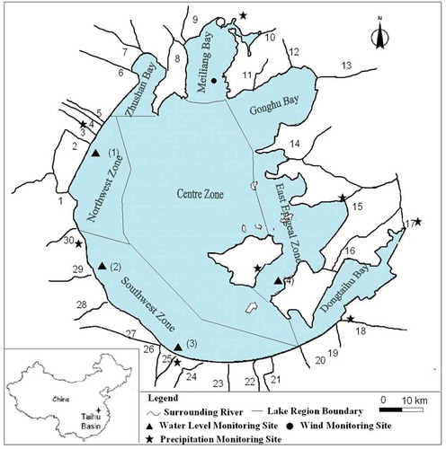
Lake Taihu, the third largest shallow freshwater lake in China, is located between 119°08ʹ–122°55ʹE and 30°05ʹ–32°08ʹN, with a surface area of 2338 km² and a catchment area of 36 500 km² (Zhu et al. 2007). The mean depth of the lake is 1.9 m and the maximum depth is 2.6 m, corresponding to an elevation of 3.0 m a.s.l. (Qin 2009). The lake bottom features flat terrain with an average topographic gradient of 0°0ʹ19.66ʺ. A shallow-water area with a mean depth of less than 1.5 m is mostly located in the eastern area and accounts for 19.3% of the total surface area. The deepest areas (>2.5 m), occupying 8.4% of the total lake area, are in the north and west. Although there is thermal stratification in Lake Taihu, it is not obvious from field observation. Its duration is usually less than one day since it is easily mixed by wind force (Zhang et al. 2008). According to field monitoring data from December 2007 to November 2008, the temperature difference from the surface to the bottom was mostly about 0–1°C, in some cases about 1–4°C and rarely over 4°C (Zhao et al. 2011a). Lake Taihu with complex shoreline geometries is connected to 172 rivers or channels (Qin 2009). The dominant wind direction on the lake is southeast in the summer and northwest in the winter, with a mean wind speed of 3.5–5 m/s (Hu et al. 2006). For convenient management and monitoring, Lake Taihu has been divided into eight sub-areas: Zhushan Bay, Meiliang Bay, Gonghu Bay, Northwest Zone, Southwest Zone, Central Zone, East Epigeal Zone and Dongtaihu Bay (Fig. 1).

Fig. 1 Location of the study area, surrounding rivers and monitoring stations in and around Lake Taihu, China. Water level monitoring stations (1)–(4) represent Dapukou, Jiapu, Xiaomeikou and Xishan, respectively.

2.2 EFDC hydrodynamic model set-up and calibration

The Environmental Fluid Dynamic Code (EFDC), a three-dimensional hydrodynamic model developed by Hamrick (1994) and Craig (2011), was utilized to simulate the water levels and currents in this study. The detailed momentum and continuity equations in the EFDC model are outlined in Hamrick (1994). The model has been extensively applied and documented for modelling circulation, thermal stratification, sediment transport, water quality and eutrophication in numerous lakes, rivers and estuaries (Li et al. 2010, 2011, Zhao et al. 2011b).

To set-up the model for Lake Taihu, rectangular grids were used containing active cells in the horizontal plane with a uniform grid. In the vertical direction, we tested different vertical layers, including one, three, five and 10 layers. The results of simulated currents and water levels showed that the vertical resolution is higher with the increase of vertical layers; however, it also increases the risk of overflow errors. As a trade-off between resolution and stability issues, a vertical sigma coordinate with an evenly distributed three-layer system was adopted herein. A previous study by Pang et al. (1994) also showed that a three-layer system in Lake Taihu describes the wind-induced current well. The currents on the surface followed the wind direction, and the flow near the bottom moved in the opposite direction to offset the surface flow (Luo and Qin 2004). Thus, in this study, a vertical sigma coordinate with an evenly distributed three-layer system was applied to effectively simulate the vertical currents. Additionally, average maximum slopes of water depth were less than 0.33, which agreed with the condition of hydrostatic consistency and avoided a pressure gradient error from the sigma transformation (Mellor et al. 1994).

The model was driven by atmospheric forcing, surface wind stress, and tributary inflow/outflow (Fig. 2). The lake is a typical large shallow lake with wind-driven currents and a lack of stratification. Therefore, temperature was treated as constant due to its minimal effect on the results of hydrodynamic processes (Li et al. 2011). Inflow and outflow tributaries included 30 primary rivers (Fig. 1). Precipitation data were obtained by averaging data from eight monitoring stations near the lake (Fig. 1, TBA 2009). The wind data came from the field monitoring. The average value of the first day of the simulation period was set as the initial condition with an assumption that the lake surface was level. A 10-s time step was used as a trade-off between computational speed and stability issues. Parameters relating to the Mellor and Yamada turbulence model (Mellor and Yamada 1982) were the same as those used in other hydrodynamic models, such as the Princeton Ocean model and the Estuary, Coastal and Ocean model (HydroQual Inc. 2001). Similarly, the non-dimensional viscosity parameter in the Smagorinsky (1963) formula was set to a constant value of 0.2. Bottom roughness height (z₀) was set to 0.02 m (HydroQual Inc. 2001) for water-level calibration.

Fig. 2 Methodology flowchart.

The simulated and observed surface elevations in 2005 at four monitoring stations, Dapukou, Jiapu, Xiaomeikou and Xishan (Fig. 1), showed mean absolute relative errors of 2.9, 3.46, 3.49 and 1.86%, respectively (Li et al. 2011). These data demonstrate that the model adequately simulated surface fluctuations due to variations in wind, precipitation and freshwater discharge. The results of current calibrations, based on data from lake-wide measurements of current on 12–14 March and 15–19 August 2005, suggested that although the model results did not agree with observations in some monitoring stations, the overall trend showed good agreement (Li et al. 2011). The model reproduced the main features of current circulation and variation vertically.

Even after calibration, the relative contributions of parameter estimate uncertainty propagating to the uncertainty in results still remained unclear. Thus it was essential to estimate parametric uncertainty and figure out which were the most sensitive parameter(s). During the parametric uncertainty and sensitivity process, the prevailing southeast wind direction in summer (June, July and August) was used and statistically analysed through field observation of wind data from Lake Taihu station over 5 years (1997–2001) (Luo et al. 2004, Qin et al. 2007, Li et al. 2011).

2.3 Methods of uncertainty and sensitivity analysis for hydrodynamic processes

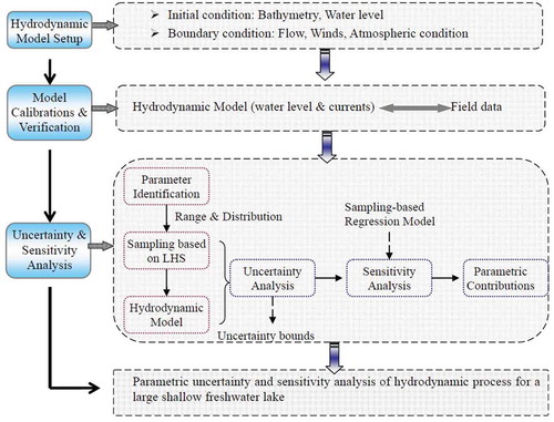
The uncertainty and sensitivity analysis of hydrodynamic processes for Lake Taihu was conducted based on LHS and the EFDC model. The analysis procedure is shown in Fig. 2 as a flowchart and may be described as follows (Helton et al. 1993, 2005):

1. Determine the probability distributions and ranges of individual parameters.

2. Generate multiple realizations of random parameters based on the estimated distributions and ranges with LHS.

3. Solve the water-level and current problems with the EFDC model for each realization.

4. Evaluate variability of output variables (e.g. water level and flow velocity at each layer).

5. Conduct a sensitivity analysis to rank the relative importance of the individual parameters to the variability of output variables.

2.3.1 Parameter identification and sampling with LHS method

2.3.1.1 Parameter identification

The hydrodynamic simulation process involves many parameters. Determining realistic and optimal values for a large number of parameters is not feasible, so reduction in the number of parameters was necessary (Muleta and Nicklow 2005). Some key input parameters were identified for further study, based on previous studies of lake hydrodynamic models (Pang et al. 1994, Luo and Qin 2004, Xu and Liu 2009, Zhou et al. 2009, Li et al. 2011), the governing equations of the EFDC hydrodynamic gmodel and the hydrodynamic characteristics of a large shallow lake. The following 10 parameters were identified for further study: wind drag coefficient, wind shelter coefficient, bottom roughness height, horizontal eddy viscosity, horizontal turbulent diffusivity, wall roughness, vertical eddy viscosity, vertical turbulent diffusivity, turbulent intensity and turbulent length scale (Table 1, Pang et al. 1994, Luo and Qin 2004, Xu and Liu 2009, Zhou et al. 2009, Li et al. 2011). These parameters were divided into five groups, i.e. air–water interface factor, surrounding terrain factor, water–sediment interface factor, turbulent diffusion parameters and turbulent intensity parameters (Table 1). The air–water interface factor and surrounding terrain factor (i.e. wind drag coefficient and wind shelter coefficient) are included in the water surface wind stress formula (Hamrick 1994, Craig 2011):

(1)

where τ_sx, τ_sy are water surface wind stress; U_w and V_w are the x and y components of the wind velocity 10 m above the water surface; c_s is the wind drag coefficient; and w_s is the wind shelter coefficient. Accurate parameterization of c_s and w_s is required to model the wind stress.

Table 1 Statistical features of the hydrodynamic parameters used for the Latin hypercube sampling method.

Parameter group	Parameters	Min	Max
Air–water interface factor	Wind drag coefficient (Cs)	5 × 10^-4	5 × 10^-3
Surrounding terrain factor	Wind shelter coefficient (ws)	0.5	1
Water–sediment interface factor	Roughness height (z0)	5 × 10^-3	5 × 10^-2
Turbulent diffusion parameters	Horizontal eddy viscosity (Hv)	1	100
	Horizontal turbulent diffusivity (Hb)	1	100
	Wall roughness (Wr)	1 × 10^-4	1 × 10^-2
	Vertical eddy viscosity (Av)	0	10
	Vertical turbulent diffusivity (Ab)	0	10
Turbulent intensity parameters	Turbulent intensity (q)	1 × 10^-5	1 × 10^-3
	Turbulent length scale (l)	1 × 10^-5	1 × 10^-3

Note The unit for roughness height (z₀) is m; while other parameters are dimensionless.

Bottom roughness height is an important factor of the water–sediment interface affecting bottom velocity, which is included in the quadratic resistance formulation of the stress at the bed given as (Hamrick 1994, Craig 2011):

(2)

where τ_bx and τ_by are bottom stress; c_b is the bottom stress coefficient; and the subscript 1 denotes bottom layer values for the horizontal velocity components. Under the assumption that the near bottom velocity profile is logarithmic at any instant of time, the bottom stress coefficient is given by (Hamrick 1994, Craig 2011):

(3)

where κ is the von Karman constant; Δ₁ is the dimensionless thickness of the bottom layer, and z₀ is the roughness height.

The turbulent diffusion parameters and turbulent intensity parameters are related to the Mellor and Yamada turbulence model (Mellor and Yamada 1982) and the Smagorinsky (1963) formula.

2.3.1.2 Sampling of input parameters with LHS method

The LHS approach creates a sequence for every possible combination of the independent input parameters and works by taking the range of each independent parameter, dividing the range by the selected realizations, rearranging the values into a random distribution, and then combining the distributions for each independent parameter (Xu and Gertner 2008). The ranges of the parameters selected for uncertainty and sensitivity analysis (Table 1) were chosen through a detailed investigation of the literature (Pang et al. 1994, Xu and Liu 2009, Zhou et al. 2009, Li et al. 2011). Due to the lack of field data for the 10 parameters in Lake Taihu, it was hard to determine the rigorous distribution characteristics of a random hydrodynamic parameter (Ye et al. 2007, Pan et al. 2009). Therefore, four different commonly-used distribution types (uniform, normal, lognormal and triangular) were selected for the 10 parameters to generate independent parameter samples in this study.

As the variable space is sampled with relatively few samples in LHS, the number of model runs can be small compared with Monte Carlo sampling. Aalderink et al. (1996) used about 100 runs with the LHS technique in their uncertainty analysis of a heavy metal model. McKay (1988) suggested that a number of simulation runs (m) equal to twice the number of uncertain parameters (k) might provide a good balance between accuracy and computational cost for models with a large number of parameters. Manache and Melching (2004) indicated that a choice of m equal to 4/3 times the number of uncertain variables usually gave satisfactory results. In this study, 100, 150, 200, 300 and 500 realizations generated by LHS were tested in order to obtain the optimal realizations for analysing the model uncertainty and sensitivity. The results showed that the sample mean and variance stabilized well after 100 realizations. The 95% confidence intervals decreased with the increase in realizations, but varied only negligibly after 150 realizations, indicating that the statistics had stabilized. Hence, 200 realizations were selected as sufficient and meaningful statistics for the uncertainty and sensitivity assessments.

Water level and flow velocity at three layers (the surface, middle and bottom) were chosen as the hydrodynamic output targets for the uncertainty and sensitivity assessments.

2.3.2 Sampling-based uncertainty and sensitivity analysis

The relationships between the input parameters (i.e. 10 parameters) and the outputs (i.e. water level and current) are nonlinear in the EFDC model, thus it is essential to transform input parameters and output data to their corresponding ranks before using the usual sampling-based regression model. That is to say, the smallest value of each variable of input and output data is ranked 1, the next largest value 2, and so on, noting that the ranking rules are consistent for both inputs and outputs. The sampling-based regression model, relating the corresponding ranks of model inputs and outputs, is constructed as (Helton 1993):

(4)

where is the estimation of output y_i with a corresponding rank from the regression model; x_ij is the ith realization of the jth model input parameters of corresponding ranks; b₀ and b_j are the rank regression coefficients of parameter x_j; ε_i is the error term; m is the number of realizations (m = 200 in this study) and k is the number of input parameters (k = 10 in this study).

The standardized rank regression model can be reformulated as (Saltelli et al. 2000, Helton et al. 2006):

(5)

where and are the mean and standard deviation of the input parameter x_j of corresponding rank; and are the mean and standard deviation of the outputs’ corresponding ranks. The coefficient is called the standardized rank regression coefficient (SRRC). The square of SRRC can be used to represent the contribution from individual input parameters to the uncertainties of output variables (Saltelli et al. 2000, Helton et al. 2006). The parameter with a larger SRRC² contributes more to the output uncertainties.

For each numerical grid, the total variance (V) of the output over m realizations is calculated via:

(6)

For the same grid, the variance () of the regression estimated output is:

(7)

The coefficient of determination (R²) is usually applied to measure the extent to which the regression model successfully accounts for the output uncertainty:

(8)

When the input parameters are independent, can be calculated by taking the variance on both sides of equation (4), which leads to:

(9)

Combining equations (5), (8) and (9) leads to:

(10)

The term represents the fractional contributions of parameter j to the output variances; R² values are in the range of zero to one; a value near one indicates that the regression model is accounting for most of the uncertainty in the observed output, and if R² > 0.7, the regression model is acceptable for sensitivity analysis (Manache and Melching 2008).

After obtaining input (10 parameters) and output pairs (water level and velocity) for all of the 200 runs, the uncertainty and sensitivity analyses were performed. From the output statistics, distributions and correlation among input and output variables one can estimate the uncertainty of the model results and identify the most sensitive parameters. In this study, the uncertainty bounds (i.e. 5th and 95th percentiles of the simulated state variables) and the variance were used as indicators of the predictive uncertainty and they provided similar information to the output distributions. Since the uncertainty bounds measured the simulated variables directly, they were considered to be more informative.

3 RESULTS

3.1 Uncertainty analysis

The mean, variance, and 5th and 95th percentiles of the simulated state variables were evaluated from 200 realizations. The results for the uniform distribution for each parameter sampling are presented first; the impact of the other three parameter distribution functions on the results of uncertainty and sensitivity analysis are presented in Section 3.3.

3.1.1 Uncertainty of water level

The results showed that the values of mean, and 5th and 95th percentile simulated water levels (Fig. 3(a)–(c)) exhibited spatial heterogeneity with respect to the wind direction, with the highest values occurring in the northwest part of the lake and the lowest values in the southeast, For example, the respective mean, and 5th and 95th percentile water levels were 3.04, 3.01 and 3.09 m in the Northwest Zone; 3.05, 3.01 and 3.10 m in Zhushan Bay; 3.01, 3.00 and 3.04 m in the Central Zone; and 2.90, 2.83 and 2.98 m in Dongtaihu Bay. Generally, the 95th percentile of water levels had the maximum gradient in the wind direction, followed by the mean and then the 5th percentile (Fig. 3(a)–(c)). The variances in water level are shown in Fig. 3(d). The greater the variance, the more uncertain the water level, due to the uncertainty of parameters in that region. The variances of water level indicated an increasing trend from the Central Zone to the Northwest Zone and the Southeast Zone, ranging from 0.01 to 0.06. Larger variances of water level occurred at Zhushan Bay, Meiliang Bay and Dongtaihu Bay, while smaller variances occurred at the Central Zone, Gonghu Bay and part of the East Epigeal Zone.

Fig. 3 (a) Mean, (b) 5th percentile, (c) 95th percentile and (d) variance of simulated water level with uniform distributions.

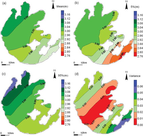
In general, it was found that uncertainty in water level was larger in bays than in open water areas, especially in semi-closed bays whose opening orientation was the same as the wind direction. This suggests that the uncertainty of water level depended on complex topography around the lake, the shape of bays and the wind fields.

3.1.2 Uncertainty of flow velocity

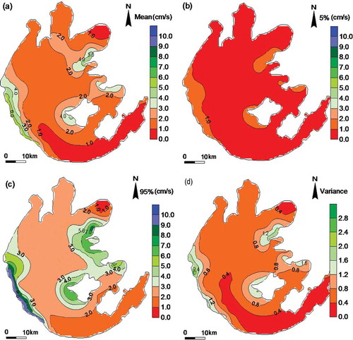
To investigate the uncertainty of velocity and its vertical distribution, the flow velocity was modelled at the surface, middle and bottom layers (Figs 4 and 5). The mean, and 5th and 95th percentiles and the variances of the surface flow velocity (Fig. 4(a)–(c)) showed a similar spatial pattern, with large velocities occurring at the Southwest littoral and East Epigeal zones. The mean values were almost twice those of the 5th percentile, and 95th percentile values were approximately four times as large as the 5th in different lake regions. However, the magnitudes of mean, and 5th and 95th percentiles were quite different. For instance, the respective values of simulated surface flow velocity were 1.59, 1.02 and 2.23 cm/s in the Northwest Zone; 1.54, 0.48 and 1.90 cm/s in Zhushan Bay; 1.22, 0.47 and 1.98 cm/s in the Central Zone; and 0.75, 0.30 and 1.23 cm/s in Dongtaihu Bay. Furthermore, the results indicated that the horizontal gradients of velocity were different. The gradients of 95th percentile flow velocity were the largest, followed by the mean, and then the 5th percentile. The spatial distribution of velocity variances (Fig. 4(d)) had a similar pattern to that of the flow velocity. For example, the maximum surface flow velocity was 10 cm/s, occurring along the littoral Southwest Zone, which also had the largest uncertainty, with a variance of about 2.4, suggesting the strong impact of parameter uncertainty on the surface flow velocity. However, there was little impact at Dongtaihu Bay, where velocities were smaller (Fig. 4). The amplitude of variances for surface flow velocity (Fig. 4(d)) and water level (Fig. 3(d)) showed that the fluctuation of variances for the surface flow velocity were markedly larger than those of water level, suggesting that the same group of model parameters exhibited different impacts on the model output.

Fig. 4 (a) Mean, (b) 5th percentile, (c) 95th percentile and (d) variance of simulated flow velocity at the surface layer with uniform distributions.

The uncertainties of the middle and bottom flow velocity were also assessed (Fig. 5). Compared with the mean flow velocity in different layers, the surface flow velocity had the maximum value, followed by the bottom flow velocity, and then the middle flow velocity (Figs 4(a), 5(a) and (c)). The velocity variances at different layers showed the same vertical patterns as the corresponding velocity patterns, with the maximum values in the surface layer and minimum values in the middle layer. Furthermore, the large variances of velocity indicated that parametric uncertainty played an important role in the predictive circulation with the hydrodynamic model.

Fig. 5 Mean and variance of simulated flow velocity: (a) and (b) at the middle layer, and (c) and (d) at the bottom layer.

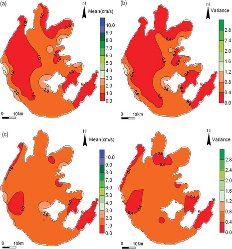
In general, the results of flow velocity in Lake Taihu suggested that: (a) the regions of the lake with a complex shoreline, near the shoreline, or with longer wind fetch had larger uncertainty; and (b) regions of the lake with a larger velocity had larger uncertainty. Hence, shoreline, geography and wind field were the most important factors in the uncertainty of flow velocity.

3.2 Sensitivity analysis

The coefficients SRRC² and R² were used to describe the relative fractional contribution of each parameter to the model outputs, and the reliability of the regression analysis in the uniform distribution case for each parameter sampling. There were two aspects to the contributions of parameter uncertainty to results uncertainty: (a) the importance of the parameter, and (b) the uncertainty of the parameter itself, which combined to determine the contribution to output uncertainty.

3.2.1 Sensitivity of water level

The R² values for the water level exceeded 0.9 in more than 84.61% of the sites, indicating that the regression analysis was generally reliable. The mean SRRC² values of wind drag coefficient over the entire lake were largest, in the range of 60–70% (Table 2), suggesting that wind drag coefficient was predominant in water-level uncertainty. This implies that the wind drag coefficient was one of the most sensitive parameters in the hydrodynamic process. The wind shelter coefficient, reflecting the surrounding terrain, also made a contribution to water-level uncertainty having SRRC² values of about 20–30% (Table 2). The wind drag and shelter coefficients represented the most dominant parameters in water-level uncertainty. In addition, the contributions of wind drag and shelter coefficients had homogeneous spatial distributions, which meant that the air–water interface and surrounding terrain factors differed little across different lake regions (Table 2). The SRRC² values of the other eight parameters (bottom roughness height, horizontal eddy viscosity, horizontal turbulent diffusivity, wall roughness, vertical eddy viscosity, vertical turbulent diffusivity, turbulent intensity and turbulent length scale) were all close to zero (not shown in Table 2), indicating that water level uncertainty was not affected by these parameters. Therefore, the general order of parameter sensitivity to water level, from the most to least important, was wind drag coefficient, wind shelter coefficient, and the other eight parameters. Since wind drag coefficient and wind shelter coefficient reflected the impact on water level of wind field and geography around the lake, the two parameters could be considered the most sensitive for water level in Lake Taihu.

Table 2 Sensitivity assessment for parameters with different distributions.

Output target	Parameter distribution	Sensitivity analysis	Gonghu Bay	Meiliang Bay	Zhushan Bay	Northwest Zone	Southwest Zone	Dongtaihu Bay	East Epigeal Zone	Central Zone
Water level	Uniform	cs SRRC^2	0.649	0.688	0.691	0.684	0.656	0.691	0.631	0.650
		ws SRRC^2	0.265	0.266	0.271	0.262	0.265	0.266	0.228	0.233
	Normal	cs SRRC^2	0.602	0.682	0.694	0.675	0.629	0.686	0.589	0.584
		ws SRRC^2	0.268	0.274	0.267	0.272	0.255	0.278	0.215	0.235
	Lognormal	cs SRRC^2	0.694	0.751	0.762	0.751	0.733	0.776	0.657	0.644
		ws SRRC^2	0.200	0.202	0.212	0.214	0.216	0.173	0.134	0.133
	Triangular	cs SRRC^2	0.688	0.752	0.752	0.745	0.688	0.760	0.663	0.667
		ws SRRC^2	0.143	0.164	0.177	0.171	0.164	0.175	0.153	0.138
Flow velocity at surface layer	Uniform	cs SRRC^2	0.701	0.679	0.725	0.670	0.643	0.646	0.706	0.671
		z0 SRRC^2	0.055	0.081	0.030	0.087	0.112	0.099	0.038	0.083
		ws SRRC^2	0.205	0.230	0.230	0.219	0.211	0.237	0.245	0.212
	Normal	cs SRRC^2	0.676	0.603	0.680	0.621	0.624	0.614	0.663	0.658
		z0 SRRC^2	0.062	0.131	0.050	0.115	0.102	0.093	0.057	0.080
		ws SRRC^2	0.228	0.227	0.242	0.224	0.223	0.246	0.254	0.229
	Lognormal	cs ^SRRC2	0.770	0.773	0.731	0.780	0.717	0.740	0.750	0.754
		z0 SRRC^2	0.054	0.056	0.046	0.066	0.120	0.048	0.067	0.065
		ws SRRC^2	0.161	0.143	0.196	0.148	0.111	0.190	0.178	0.152
	Triangular	cs SRRC^2	0.772	0.707	0.774	0.722	0.708	0.685	0.750	0.746
		z0 SRRC^2	0.051	0.100	0.041	0.096	0.100	0.098	0.046	0.073
		ws SRRC^2	0.160	0.163	0.167	0.165	0.152	0.162	0.172	0.165

3.2.2 Sensitivity of flow velocity

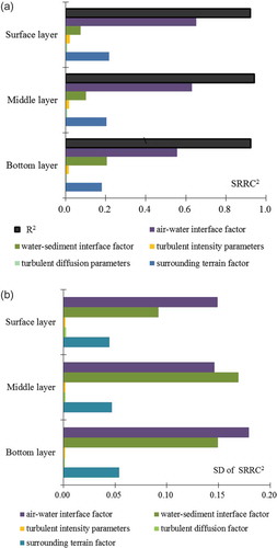
The spatial distribution of SRRC² values for 10 parameters on the flow velocity uncertainty and R² of regression analysis at each layer were calculated. The R² values at the surface layer exceeded 0.9 in over 95% sites, suggesting that the regression analysis was reliable. The SRRC² values for wind drag coefficient were largest, in the range of 65–70% in the lake, with peak values occurring in Zhushan Bay with a large wind fetch (Table 2). It illustrates that the flow velocity uncertainty at the surface layer was largely controlled by wind drag coefficient uncertainty, which was consistent with the results of water-level uncertainty. In other words, the wind drag coefficient was the most important parameter for flow velocity uncertainty in Lake Taihu. The SRRC² values of wind shelter coefficient for velocity were the second largest; their contribution was about 20% in most regions of the lake (Table 2). The SRRC² values of roughness height were approximately equal to or slightly smaller than those for wind shelter ranging from 3 to12%. The SRRC² values of turbulent diffusion and turbulent intensity parameters were close to zero in most regions, indicating that flow velocity uncertainty was insensitive to these seven parameters. These results agree with previous literature in which the seven parameters were set to be constant (Xu and Liu 2009, Zhou et al. 2009, Li et al. 2011). In general, important parameter groups for the uncertainty of surface velocity were in the descending order: air–water interface factor (60–75%), surrounding terrain factor (20%), water–sediment interface factor (3–12%), turbulent diffusion parameters (<1%) and turbulent intensity parameters (<1%).

The mean and standard deviation of SRRC² of the 10 parameters on flow velocity at the middle and bottom layers were calculated. The mean R² values were, as in the surface layer, in excess of 0.9 for the middle and bottom layer flow velocity (Fig. 6(a)). Among the 10 parameters affecting the flow velocity at different layers, the mean SRRC² values for wind drag coefficient and wind shelter coefficient were the largest for all three layers, suggesting that the parametric uncertainties in the air–water interface factor and surrounding terrain factor were the largest contributors to the flow velocity uncertainty. The contributions of parametric uncertainty in wind drag coefficient and wind shelter coefficient to flow uncertainty varied with the layers from 55 to 65% and from 18 to 22%, respectively (Fig. 6(a)), and decreased gradually in the vertical direction from surface to bottom layers. The mean SRRC² values of roughness height were the third largest in the three layers, in the range of 10–20% (Fig. 6(a)). It was also found that SRRC² of roughness height increased gradually from the surface to the bottom layers. The results suggested that the surface flow velocity was dominated by the air–water interface factor and surrounding terrain factor, while the bottom velocity was co-dominated by air–water, water–sediment interface parameters and surrounding terrain parameter. The means of SRRC² for turbulent diffusion parameters and turbulent intensity parameters were less than 1% for all layers (Fig. 6(a)), indicative of the limited contributions of their uncertainty to flow velocity in all layers. The standard deviation of SRRC² was large for the wind drag coefficient, wind shelter coefficient and roughness height for all layers, which indicated the spatial variation of sensitivity of flow velocity to the three parameters within each layer (Fig. 6(b)). For a large shallow lake, the uncertainty of flow velocity was largely caused by the uncertainty of wind, surrounding terrain and roughness height parameters, while the contributions to the velocity in different lake regions varied more than water level (Table 2).

Fig. 6 Mean and standard deviation (SD) of standardized regression coefficient (SRRC²) of the five parameters for flow velocity uncertainty at different vertical layers with a uniform distribution.

3.3 Impact of parameter probability density functions

The mean values and variances of output from four different distributions of input parameters, including uniform, normal, lognormal and triangular distribution cases, were compared to investigate the impact of the probability density functions of the input parameters on the uncertainty and sensitivity of hydrodynamic processes in the large shallow lake from the EFDC model.

For the distributions considered, the mean water levels had a similar pattern and magnitude. The largest values of mean water level in all the cases occurred in the same bays (i.e. Zhushan Bay and Meiliang Bay) with a long wind fetch, while the smallest values occur in Dongtaihu Bay with a short wind fetch. The variances of water level also had similar ranges with different distributions. For flow velocity, further analysis revealed similar results when different parameter distributions were used.

The most sensitive parameters to water level were wind drag coefficient and wind shelter coefficient when different distributions were used (Table 2). For the surface flow velocity, the three most sensitive parameters were wind drag coefficient, wind shelter coefficient and roughness height coefficient in all cases (Table 2). The lake regions with long wind fetch (e.g. Zhushan Bay) were relatively strongly impacted, largely by wind drag coefficient and wind shelter coefficient. Although the parameters had slightly different contributions to lake area in the case of different parameter distributions, the order for sensitivity of parameters and the magnitude for the contributions of parameters remained consistent.

Overall, there were no obvious changes in the uncertainty and sensitivity of hydrodynamic processes simulated by the EFDC model in Lake Taihu assuming different parameter distributions.

4 DISCUSSION

4.1 Parametric uncertainty and sensitivity assessment of hydrodynamic process

The results showed that, in the hydrodynamic model, those parameters associated with wind field and bottom roughness contributed greatly (over 80%) to the uncertainty of the hydrodynamic process in Lake Taihu. It was suggested that when calibrating and validating the hydrodynamic process for a large shallow lake, wind drag coefficient, wind shelter coefficient and bottom roughness height should be taken into account and treated carefully.

When winds passed over the lake, the water level at the downwind end of the lake would rise. The term wind set-up referred to the slope of the water surface in the direction of the wind stress (Francis 1959). The spatial distribution of water level in Lake Taihu increased from southeast to northwest under the driving force of a constant southeast wind, suggesting that winds help alter water levels in Lake Taihu by piling water up on the northwest side while lowering water levels on the southeast side. The uncertainty of water level exhibited various spatial patterns with large uncertainty occurring in both the northwest region with a high water level and the southeast region with a low water level, which may be due to the duration, direction and speed of the wind and the length, shape and depth of the different lake regions. Fagherazzi and Wiberg (2009) also pointed out that wind condition has a significant impact on the hydrodynamic process (water level, shear stress) in shallow intertidal basins. The impact of winds on the hydrodynamic processes can be explained by the wind fetch, which is the length of a lake along a certain direction, describing the longest distance an air mass can travel across a lake. In most lakes, the fetch determines the size of water level set-up, current and waves. Winds travelling over a long fetch are able to cause significant changes in water level (Carniello et al. 2011). In Lake Taihu, winds travelled a relatively long distance when arriving at a northwest lake region such as Zhushan Bay and Meiliang Bay under the prevailing southeasterly wind, resulting in a large water level set-up and high uncertainty in those regions. The decrease of water level was relatively small in Dongtaihu Bay due to its small wind fetch (Luo and Qin 2003, 2004, Qin et al. 2007). However, the uncertainties of simulated water level in Dongtaihu Bay were very high, which was perhaps due to the complex shorelines in this region. In general, wind was the main driving force for the changes of water level in Lake Taihu.

In the lake circulation model, wind drag coefficient, wind shelter coefficient and bottom roughness height predominated, contributing greatly to the uncertainty of flow velocity. The spatial distribution of uncertainty in velocity showed a similar pattern to that of velocity in the lake. For example, large uncertainties occurred in the same area as large velocities. Vertically, the uncertainty of flow velocity in the surface layer was largest, followed by the bottom layer and the middle layer in most regions. This may be due to the comprehensive effect of bottom roughness and wind parameters. Bottom roughness height contributed more to the bottom layer velocity, while wind drag coefficient and wind shelter coefficient contributed more to the surface and middle layer velocity. Additionally, a large portion of the wind energy affected the surface flow field, although some could reach the bottom after the energy is transformed to waves and current and produce turbulent fluctuations (Bengtsson and Hellström 1992). The smallest uncertainty in the middle layer was as a result of the combined interaction of the air–water interface and water–sediment friction. Thus, the wind field, in combination with bottom roughness height, determined the circulation pattern in Lake Taihu.

In general, the uncertainty and sensitivity analysis results suggested that wind drag coefficient, wind shelter coefficient and roughness height were the most important driving factors for the hydrodynamic process in Lake Taihu. This could be regarded as typical for a similar large shallow lake. However, these parameters may not always be the dominating and sensitive factors for deep lakes and channel-rivers and lakes. As deep lakes have relatively lower surface-to-volume ratios in comparison with shallow ones, this restricts the interaction of the water body with the atmosphere, bottom sediments and the surrounding land (Kroes 1986, Read et al. 2011). In deep lakes, the hydrodynamic processes will be distinctly different between the surface layer, the interior of the density-stratified deep water, and the bottom layer. According to previous studies (Tsvetova 1999, Li et al. 2011), the hydrodynamic process in surface water in deep lakes is dominated by parameters related to wind and atmospheric conditions, similar to shallow lakes. However, the hydrodynamic processes in the middle and bottom water are mostly controlled by thermal structure (e.g. thickness of active bed temperature layer) to form density currents. This might mean that the parameters relating to those driving forces are sensitive for deep lake hydrodynamic models. Additionally, for channel-rivers and lakes, due to complex morphology, it is essential to calibrate bottom roughness in different channel sections (Ran et al. 2010). For example, Zhao et al. (2003) carefully calibrated bottom roughness height instead of wind parameters, by settling on a range of 0.022–0.011 m from upstream to downstream and 0.08–0.04 m near the central island to effectively improve flow velocity accuracy in part of the Yangtze River Model. Therefore, it is important to identify the major driving factors and sensitive parameters when developing different types of lake hydrodynamic models.

4.2 Wind data preparation for lake hydrodynamic model

Our results showed that wind was the most important impact factor for hydrodynamic processes in Lake Taihu. Hence, it was essential to provide the appropriate input data of wind for the model. In previous studies, the dominant wind magnitude and direction in summer or winter in the study area was applied for the whole model computation domain, without considering the temporal and spatial variation of the winds. Others fed the lake model with observed wind data from one or two monitoring stations located in or around the lake, without analysing the representativeness of that data (Wang et al. 2001). Wang et al. (2010) found that the wind field around Lake Taihu showed high temporal and spatial heterogeneity based on 7 years of observed data from 17 meteorological stations. Therefore, the spatial variability of the wind field should be taken into account when setting up a hydrodynamic model for a large shallow lake.

Besides the wind data, the wind drag coefficient and wind shelter coefficient should be as accurate as possible. However, the wind drag coefficient has often been taken as a constant over the whole domain, or expressed as various functions about the wind velocity 10 m above the water surface (Zhou et al. 2009). Although these methods have been widely used in numerical simulations, they may have relatively low accuracy. Chen et al. (2008) provides a good method to calculate the spatial wind drag coefficient using the adjoint data assimilation model. Geernaert et al. (1986) found that variations in the magnitude of the drag coefficient could be explained by coincident variations in the surface wave energy spectrum. In addition, another important wind parameter, the wind shelter coefficient, was ignored when developing a hydrodynamic model. However, complicated terrain around a lake, such as mountains, often results in an asymmetrical distribution of wind velocity and direction above the lake surface, which would affect flow patterns in the lake. For example, Li et al. (1998) examined the impact of wind shelter of hilly terrains on the circulation pattern by a 2-D wind-driven current model of Dianchi Lake and a 3-D micrometeorology model, and found that using spatially variable wind shelter coefficients improved the simulation precision of the model. Hence, the spatial wind field should be considered when setting up hydrodynamic and transport models of sediments, nutrients, and algae to reduce the uncertainty.

4.3 Impact of parameter probability density functions

When sampling multiple random variables in the model by LHS, the distribution function of parameters may affect the uncertainty results. Most previous work assumed a uniform distribution for each parameter when experimental data were limited (Muleta and Nicklow 2005, Xu and Gertner 2008). Some work assumed that the a priori distribution was uniform and then used Bayesian methods to update the posterior distribution of the parameters, which exhibited different patterns. In this study, uncertainty and sensitivity results of hydrodynamic processes, based on four common distributions for the major parameters, showed no clear differences between different distributions (Table 2). This suggests that one could choose the uniform distribution instead of other complex distributions for uncertainty analysis in a large shallow lake when there are insufficient experimental data.

5 CONCLUSIONS

In this study, parametric uncertainty and sensitivity analysis were conducted for hydrodynamic processes of a large shallow lake using a combination of the EFDC model and the LHS method. The distribution functions of the parameters (e.g. uniform, normal, lognormal and triangular) were found to have little impact on the uncertainty and sensitivity of hydrodynamic processes in Lake Taihu. The degree of uncertainty for the Lake Taihu hydrodynamic model was highly associated with parametric uncertainties. In particular, the uncertainties in wind drag coefficient, wind shelter coefficient and roughness height were the most important contributing factors to hydrodynamic process uncertainties (60–70%, about 20% and 10%, respectively). Turbulent diffusion and turbulent intensity parameters (including seven parameters) only had a slight impact on the hydrodynamic process, with a contribution of less than 1%. Therefore, for a large shallow lake hydrodynamic model, attention should be paid to the shoreline and geography, and the parameters relating to wind and roughness. Since this paper only addressed the parametric uncertainty and sensitivity for the hydrodynamic processes in a large shallow lake, the uncertainty and sensitivity from boundary conditions (e.g. wind fields and flow boundary) should be studied further.

Disclosure statement

No potential conflict of interest was reported by the author(s).

Additional information

Funding

The research was supported by the Chinese National Science Foundation (51379061, 51179053, and 41323001), and Jiangsu Province Science Foundation (BK20131370). The research was also supported by the Programme for Excellent Talents in Hohai University, and Qing Lan Project.

REFERENCES

- Aalderink, R.H., et al., 1996. Effect of input uncertainties upon scenario predictions for the River Vecht. Water Science and Technology, 33 (2), 107–118. doi:10.1016/0273-1223(96)00193-X.
- Bengtsson, L. and Hellström, T., 1992. Wild-induced resuspension in a small shallow lake. Hydrobiologia, 241 (3), 163–172. doi:10.1007/BF00028639.
- Carniello, L., D’Alpaos, A., Defina, A., 2011. Modeling wind waves and tidal flows in shallow micro-tidal basins. Estuarine Coastal and Shelf Science, 92 (2), 263–276. doi:10.1016/j.ecss.2011.01.001.
- Chapra, S., et al., 2007. QUAL2K: a modeling framework for simulating river and stream water quality version 2.07: documentation and user’s manual. Medford, MA: Civil and Environmental Engineering Department, Tufts University.
- Chen, Y.D., et al., 2008. Inversing wind drag coefficient by the adjoint data assimilation method. Journal of Nanjing Institute of Meteorology, 31 (6), 879–882 (in Chinese).
- Craig, P.M., 2011. User’s manual for EFDC_Explorer: a pre/post processor for the environmental fluid dynamics code. Knoxville, TN: Dynamic Solutions-International, LLC.
- Cryer, S.A. and Havens, P.L., 1999. Regional sensitivity analysis using a fractional factorial method for the USDA model GLEAMS. Environmental Modelling & Software, 14 (6), 613–624. doi:10.1016/S1364-8152(99)00003-1.
- DHI, 2003. MIKE 11: a modeling system for rivers and channels: short introduction tutorial. Hørsholm, Denmark: DHI Software.
- Fagherazzi, S. and Wiberg, P.L., 2009. Importance of wind conditions, fetch, and water levels on wave-generated shear stresses in shallow intertidal basins. Journal of Geophysical Research – Earth Surface, 114 (F3), F03022. doi:10.1029/2008JF001139.
- Francis, J.R.D., 1959. Wind action on a water surface. ICE proceedings, 12 (2), 197–216. doi:10.1680/iicep.1959.12126
- Geernaert, G.L., et al., 1986. Variation of the drag coefficient and its dependence on sea state. Journal of Geophysical Research-Ocean, 91 (C6), 7667–7679. doi:10.1029/JC091iC06p07667.
- Hamrick, J.M., 1994. Application of the EFDC environmental fluid dynamics computer code to SFWMD water conservation area 2A. Williamsburg, VA: J.M. Hamrick and Associates, Report JMH-SFWMD-94-01, 126pp.
- Helton, J.C., 1993. Uncertainty and sensitivity analysis techniques for use in performance assessment for radioactive waste disposal. Reliability Engineering & System Safety, 42 (2–3), 327–367. doi:10.1016/0951-8320(93)90097-I.
- Helton, J.C. and Davis, F.J., 2002. Illustration of sampling-based methods for uncertainty and sensitivity analysis. Risk Analysis, 22 (3), 591–622. doi:10.1111/0272-4332.00041.
- Helton, J.C., Davis, F.J., and Johnson, J.D., 2005. A comparison of uncertainty and sensitivity analysis results obtained with random and Latin hypercube sampling. Reliability Engineering & System Safety, 89 (3), 305–330. doi:10.1016/j.ress.2004.09.006.
- Helton, J.C., et al., 2006. Survey of sampling-based methods for uncertainty and sensitivity analysis. Reliability Engineering & System Safety, 91 (10–11), 1175–1209. doi:10.1016/j.ress.2005.11.017.
- Hu, W.P., et al., 2006. A vertical-compressed three-dimensional ecological model in Lake Taihu, China. Ecological Modelling, 190 (3–4), 367–398. doi:10.1016/j.ecolmodel.2005.02.024.
- HydroQual Inc, 2001. A primer for ECOMSED version 1.2: user manual. Mahwah, NJ: HydroQual, Inc.
- Jacques, J., Lavergne, C., and Devictor, N., 2006. Sensitivity analysis in presence of model uncertainty and correlated inputs. Reliability Engineering & System Safety, 91 (10–11), 1126–1134. doi:10.1016/j.ress.2005.11.047.
- Kroes, H.W., 1986. Restoration of shallow lake ecosystems, with emphasis on Loosdrecht Lakes. Hydrobiological Bulletin, 20 (1–2), 5–7. doi:10.1007/BF02291145.
- Li, S.J., et al., 1998. Numerical simulation of influence of hilly relief on wind-driven current in Dianchi Lake. Journal of Lake Sciences, 10 (1), 5–10 (in Chinese).
- Li, Y.P., et al., 2010. Modeling water ages and thermal structure of Lake Mead under changing water levels. Lake and Reservoir Management, 26 (4), 258–272. doi:10.1080/07438141.2010.541326.
- Li, Y.P., et al., 2011. Modeling impacts of Yangtze River water transfer on water ages in Lake Taihu, China. Ecological Engineering, 37 (2), 325–334. doi:10.1016/j.ecoleng.2010.11.024.
- Luo, L.C. and Qin, B.Q., 2003. Numerical simulation based on a three-dimensional shallow-water hydrodynamic model in Lake Taihu-Current circulations in Lake Taihu with prevailing wind-forcing. Journal of Hydrodynamics. Ser. A, 18 (6), 686–691 (in Chinese).
- Luo, L.C. and Qin, B.Q., 2004. Three-dimensional numerical simulations of wind-induced circulation in Lake Taihu. Journal of Hydrodynamics, Ser. B, 16 (3), 341–349 (in Chinese).
- Manache, G. and Melching, C.S., 2004. Sensitivity analysis of a water-quality model using Latin hypercube sampling. Journal of Water Resources Planning and Management, 130 (3), 232–242. doi:10.1061/(ASCE)0733-9496(2004)130:3(232).
- Manache, G. and Melching, C.S., 2008. Identification of reliable regression- and correlation-based sensitivity measures for importance ranking of water quality model parameters. Environmental Modelling & Software, 23 (5), 549–562. doi:10.1016/j.envsoft.2007.08.001.
- McKay, M.D., 1988. Sensitivity and uncertainty analysis using statistical sample of input values. In: Y. Ronen, ed. Uncertainty analysis. Boca Raton, FL: CRC Press, 145–186.
- Mckay, M.D., et al., 1979. A comparison of three methods for selecting values of input variables in the analysis of output from a computer code. Technometrics, 21 (2), 239–245.
- Mellor, G.L., Ezer, T., and Oey, L., 1994. The pressure gradient conundrum of sigma coordinate ocean models. Journal of Atmospheric and Oceanic Technology, 11 (4), 1126–1134. doi:10.1175/1520-0426(1994)011<1126:TPGCOS>2.0.CO;2.
- Mellor, G.L. and Yamada, T., 1982. Development of a turbulence closure model for geophysical fluid problems. Reviews of Geophysics, 20 (4), 851–875. doi:10.1029/RG020i004p00851.
- Morris, M.D., 1991. Factorial sampling plans for preliminary computational experiments. Technometrics, 33 (2), 161–174. doi:10.1080/00401706.1991.10484804.
- Muleta, M.K. and Nicklow, J.W., 2005. Sensitivity and uncertainty analysis coupled with automatic calibration for a distributed watershed model. Journal of Hydrology, 306 (1–4), 127–145. doi:10.1016/j.jhydrol.2004.09.005.
- Munoz-Carpena, R., Fox, G.A., and Sabbagh, G.J., 2010. Parameter importance and uncertainty in predicting runoff pesticide reduction with filter strips. Journal of Environmental Quality, 39 (2), 630–641. doi:10.2134/jeq2009.0300.
- Pan, F., et al., 2009. Numerical evaluation of uncertainty in water retention parameters and effect on predictive uncertainty. Vadose Zone Journal, 8 (1), 158–166. doi:10.2136/vzj2008.0092.
- Pan, F., et al., 2011. Sensitivity analysis of unsaturated flow and contaminant transport with correlated parameters. Journal of Hydrology, 397 (3–4), 238–249. doi:10.1016/j.jhydrol.2010.11.045.
- Pang, Y., et al., 1994. Numerical simulations and their verification with nonuniform wind stress in Taihu Lake. Tansactions of Oceanology & Limnology, 4, 9–15 (in Chinese).
- Qin, B.Q., 2009. Process and prospect on the eco-environmental research of Lake Taihu. Journal of Lake Sciences, 21 (4), 445–455 (in Chinese).
- Qin, B.Q., et al., 2007. Environmental issues of Lake Taihu, China. Hydrobiologia, 581, 3–14. doi:10.1007/s10750-006-0521-5.
- Ran, L., Wang, S., and Fan, X., 2010. Channel change at Toudaoguai Station and its responses to the operation of upstream reservoirs in the upper Yellow River. Journal of Geographical Sciences, 20 (2), 231–247. doi:10.1007/s11442-010-0231-9.
- Read, J.S., et al., 2011. Derivation of lake mixing and stratification indices from high-resolution lake buoy data. Environmental Modelling & Software, 26 (11), 1325–1336. doi:10.1016/j.envsoft.2011.05.006.
- Saltelli, A., et al., 2000. Sensitivity analysis. Chichester: John Wiley & Sons.
- Saltelli, A., et al., 2008. Global sensitivity analysis: The Paimer. Chichester: John Wiley & Sons.
- Smagorinsky, J., 1963. General circulation experiments with the primitive equations: I. The basic experiment. Monthly Weather Review, 91 (3), 99–164. doi:10.1175/1520-0493(1963)091<0099:GCEWTP>2.3.CO;2.
- Straten, G.T. and Keesman, K.J., 1991. Uncertainty propagation and speculation in projective forecasts of environmental change: a lake-eutrophication example. Journal of Forecasting, 10 (1–2), 163–190. doi:10.1002/for.3980100110.
- TBA Taihu Basin Authority of Ministry of Water Resources, Shanghai, China, 2009. Database of water diversion from Yangtze River to Lake Taihu [online]. Available from: http://www.tba.gov.cn/ztbd/yjjt/xyfx/yq detail th.asp. [Accessed 15 August].
- Tsvetova, E.A., 1999. Mathematical modelling of Lake Baikal hydrodynamics. Hydrobiologia, 407, 37–43. doi:10.1023/A:1003766220781.
- USEPA, 2011. United States Environmental Protection Agency: Hydrodynamic models [online]. Available from: http://www.epa.gov/athens/wwqtsc/html/hydrodynamic_models.html [Accessed 17 November, 2011].
- Van, G. and Meixner, T., 2006. Methods to quantify and identify the sources of uncertainty for river basin water quality models. Water Science and Technology, 53 (1), 51–59. doi:10.2166/wst.2006.007.
- Wang, C.L., et al., 2010. Divergence characteristics and formation mechanism of wind field appropriate for the cyanbacteria bloom in Taihu Lake. China Environment and Science, 30 (9), 1168–1176 (in Chinese).
- Wang, H.Z., et al., 2001. A quasi-3D numerical model of wind-driven current in Taihu Lake considering the variation of vertical coefficient of eddy viscosity. Journal of Lake Sciences, 13 (3), 233–239 (in Chinese).
- Wool, T.A., et al., 2007. Water Quality Analysis Simulation Program (WASP) version 6.0 draft: user’s manual. Atlanta, GA: US Environmental Protection Agency–Region 4.
- Wüest, A. and Lorke, A., 2003. Small-scale hydrodynamics in lakes. Annual Review of Fluid Mechanics, 35, 373–412. doi:10.1146/annurev.fluid.35.101101.161220.
- Xu, C.G. and Gertner, G.Z., 2008. Uncertainty and sensitivity analysis for models with correlated parameters. Reliability Engineering & System Safety, 93 (10), 1563–1573. doi:10.1016/j.ress.2007.06.003.
- Xu, X.F. and Liu, Q.Q., 2009. Numerical study on the characteristics of wind-induced current in Taihu Lake. Chinese Journal of Hydrodynamics, 24 (4), 512–518 (in Chinese).
- Ye, M., et al., 2007. Assessment of radionuclide transport uncertainty in the unsaturated zone of Yucca Mountain. Advances in Water Resources, 30 (1), 118–134. doi:10.1016/j.advwatres.2006.03.005.
- Zhang, Y.C., et al., 2008. Field Measurement and analysis on diurnal stratification in Taihu Lake. Environmental Science and Management, 33 (6), 117–121.
- Zhao, D.H., et al., 2003. 2-D depth-averaged follow-pollutions model for Jiangsu reaches in Yangtze River. Shuili Xuebao, 6, 72–77 (in Chinese).
- Zhao, L., et al., 2011a. Thermal stratification and its influence factors in a large-sized and shallow Lake Taihu. Advance in water science, 22 (6), 845–850 (in Chinese).
- Zhao, X., et al., 2011b. Key uncertainty sources analysis of water quality model using the first order error method. International Journal of Environmental Science and Technology, 8 (1), 137–148. doi:10.1007/BF03326203.
- Zhou, J., et al., 2009. Influence of wind drag coefficient on wind-drived flow simulation. Chinese Journal of Hydrodynamics, 24 (4), 440–447 (in Chinese).
- Zhu, G.W., et al., 2007. Effects of hydrodynamics on phosphorus concentrations in water of Lake Taihu, a large, shallow, eutrophic lake of China. Hydrobiologia, 194, 53–61. doi:10.1007/978-1-4020-6158-5_6.