Dependence between flood peaks and volumes: a case study on climate and hydrological controls

Abstract

The aim of this paper is to understand the causal factors controlling the relationship between flood peaks and volumes in a regional context. A case study is performed based on 330 catchments in Austria ranging from 6 to 500 km² in size. Maximum annual flood discharges are compared with the associated flood volumes, and the consistency of the peak–volume relationship is quantified by the Spearman rank correlation coefficient. The results indicate that climate-related factors are more important than catchment-related factors in controlling the consistency. Spearman rank correlation coefficients typically range from about 0.2 in the high alpine catchments to about 0.8 in the lowlands. The weak dependence in the high alpine catchments is due to the mix of flood types, including long-duration snowmelt, synoptic floods and flash floods. In the lowlands, the flood durations vary less in a given catchment which is related to the filtering of the distribution of all storms by the catchment response time to produce the distribution of flood producing storms.

Editor Z.W. Kundzewicz

Résumé

Le but de cet article est d’identifier les facteurs contrôlant la relation entre pics et volumes de crues dans un contexte régional. Une étude de cas a été réalisée sur la base de 330 bassins versants autrichiens, dont les superficies allaient de 6 à 500 km². Les débits des crues maximales annuelles ont été comparés aux volumes de crue associés et la qualité de la relation pic–volume a été quantifiée par le coefficient de corrélation de rang de Spearman. Les résultats indiquent que les facteurs liés au climat contrôlent davantage la qualité de la relation que les facteurs liés au bassin. Les coefficients de corrélation de rang de Spearman vont généralement d’environ 0,2 pour les bassins de haute montagne à environ 0,8 en plaine. Le faible lien observé pour les bassins de haute montagne est dû à la diversité des types de crues, incluant des crues prolongées de fonte des neiges, des crues à l’échelle synoptique et des crues soudaines. En plaine, les durées de crue varient moins dans un bassin donné, ce qui est lié au filtrage de la distribution de tous les événements de précipitation par le temps de réponse du bassin versant pour produire la distribution des événements générant des crues.

Key words:

• flood peak
• flood volume
• consistency
• correlation
• flood types
• hydrological processes
• regional analysis
• comparative hydrology
• Austria

Mots clefs:

• pic de crue
• volume de crue
• cohérence
• corrélation
• types de crues
• processus hydrologiques
• analyse régionale
• hydrologie comparative
• Autriche

INTRODUCTION

Although both flood peaks and volumes are needed for many practical applications in hydrology, surprisingly little research has been devoted to their joint characteristics. Most of the research has focused on the flood peaks alone, in particular on extreme value distributions. Yet, the design of retention basins and spillways of reservoirs, as well as other hydraulic structures where storage is involved, requires not only peak discharges but the entire hydrograph, or at least volume estimates, in order to calculate the effect of the inflow on the storage, and therefore failure probabilities. Similarly, the relationship between flood peaks and volumes is an intriguing scientific research issue in its own right, in particular the interplay of climatic and catchment processes in defining the probabilities of peaks and volumes.

In practice, flood peaks and volumes are often dealt with in a multivariate frequency framework. Traditionally, identical marginal distributions for both random variables have been used (e.g. Sackl and Bergmann 1987, Goel et al. 1998, Yue et al. 2002), but, more recently, copulas have attracted a lot of attention as they allow for more flexibility in the marginal distributions and the dependence between peaks and volumes (e.g.  Grimaldi and Serinaldi 2006, Chowdhary et al. 2011, Bačová-Mitková and Halmová 2014). There have been numerous studies on the degree of the dependence between peaks and volumes (e.g. Shiau 2003, De Michele et al. 2005, Chen et al. 2010, Zegpi and Fernández 2010, Salvadori et al. 2011, Gräler et al. 2013, Requena et al. 2013, Serinaldi and Kilsby 2013) that is needed to estimate the multivariate quantiles and the choice of the copula function (e.g. Favre et al. 2004, Genest and Favre 2007, Chowdhary et al. 2011). Most of the literature, however, treats the dependence from a purely statistical perspective. It would be of interest to understand the hydrological factors controlling the strength of association between peaks and volumes. This would assist in the choice of the copula function to go beyond statistics alone. The additional information is important as there are rarely enough data to reliably fit copula models of peaks and volumes for large return periods. Bivariate models (of peak and volume) are much more data hungry than univariate models of peaks alone, so a priori information on causal factors is essential.

At a basic level it is clear that flood volumes of convective events lasting only for a few hours will be smaller than volumes from frontal rain or snowmelt induced floods that may last for days or weeks. At a more quantitative level, flood volumes can be related to (a) the time scales of the meteorological inputs (rainfall, snowmelt) and (b) the times scales of the storage and delay of this input in the catchment, both on the hillslopes and in the channels (Viglione et al. 2010a, 2010b). The meteorological inputs and the catchment delay control the relationship between the peaks and volumes, in terms of both their trend and the scatter around that trend. Viglione and Blöschl (2009) and Gaál et al. (2012) derived relationships between peaks and volumes and argued that the catchment acts as a filter, so storm durations similar to the response time scale of the catchment lead to larger floods than shorter and longer storm durations.

Meteorological or climatic inputs are often used to classify floods into flood types. Hirschboeck et al. (2000) classified floods into tropical, convective and frontal events based on surface and upper weather maps. Merz and Blöschl (2003) classified floods into long-rain floods, short-rain floods, flash floods, rain-on-snow floods and snowmelt floods based on an analysis of the climatic inputs (rainfall, snowmelt) and the catchment state (soil moisture, snow). One would expect the flood types to have a bearing on the dependence between peaks and volumes. Renard and Lang (2007), for example, identified snowmelt and rain-fed floods for the Ubaye River in southeastern France and showed that, for snow-related events, peak flows and volumes were more correlated than for rain-fed floods. They suggested that modelling the dependence with a single correlation parameter may lead to poor results if more than one flood type is present.

The other important set of controls is related to catchment processes. Catchment response times are usually related to the hydraulic relationships of the land surface of the catchment to represent overland flow (e.g. Dooge 2005, Pavelková et al. 2012), or to bulk properties of the catchment to represent a wider array of processes (McCuen et al. 1984, Sheridan 1994, Melone et al. 2002, Fang et al. 2005), including the hydrogeology (Gaál et al. 2012). Such relationships tend to be specific to the hydrological regime they have been derived for. However, exploring these factors in the context of regional process knowledge allows one to advance the understanding of catchment response for situations that are too complex or data-scarce to be reliably captured by distributed models (Blöschl 2006, Blöschl and Merz 2009). Flow resistance may be indexed by land-use, urbanization, or a storage parameter (Folmar et al. 2007); water input may be indexed by rainfall depth (Rao et al. 1972); and landscape evolution processes may be related to catchment attributes, such as drainage density and the hypsometric form of the catchment (Harlina 1984, Corradini et al. 1995). These processes will all affect the relationship between flood peaks and volumes in some way.

While several previous studies have examined individual factors controlling the relationship between flood peaks and volumes, this has rarely been done in a regional context. Yet, a regional analysis of the controls, based on the concept of comparative hydrology (Falkenmark and Chapman 1989), can provide interesting insights into the factors by contrasting similarities and dissimilarities between catchments (Blöschl et al. 2013a). The aim of this paper is to explore the relationship between flood peaks and volumes from a regional perspective, to understand (a) how closely peaks and volumes are related and (b) the causal factors of the consistency of this relationship.

The paper studies the peak–volume relationships for the region of Austria, which features a diverse spectrum of hydrological flood processes and has been well studied in the past (e.g. Merz and Blöschl 2003, Merz et al. 2006, Merz and Blöschl 2009, Gaál et al. 2012). Specifically, the paper builds on Gaál et al. (2012), who examined the average dependence of volumes and peaks in terms of their ratio, termed the average flood time scale. They showed that these flood time scales were controlled both by climatic factors (storm types and the antecedent soil moisture) and by the geology and land form. When expressed in a graphical way, the average flood time scales correspond to the slope of the peak–volume relationship, as shown schematically in Fig. 1 (right). In contrast, this paper is concerned with the scatter in these plots, i.e. how consistent this relationship is between events. The top panel of Fig. 1 shows a catchment where the peak–volume relationship is consistent, while the opposite case is shown in the bottom panel. The paper explores whether this consistency is related to the consistency of the climatic driving flood processes or flood types. Generally, flash floods are associated with small volumes, synoptic floods with bigger volumes, and snowmelt floods with even bigger volumes, in particular in alpine areas.

Fig. 1 Schematic of flood peak–volume relationships. Top: consistent relationship (strong type of association). Bottom: not consistent relationship (weak type of association).

The closeness of the relationship is expressed by Spearman rank correlation coefficient between flood peaks and the associated flood volumes. The focus is on maximum annual floods as this is the dataset for which the flood typology of Merz and Blöschl (2003) has been derived in the study region.

The paper is structured as follows. First, the study region is characterized from both climatological and hydrological points of view, followed by a description of the rainfall and runoff data used for the current study. The Methods section explains how flood volumes were estimated from the runoff records, how peak volume relationships were analysed, and how the flood seasonality was calculated. The Results section presents findings on the effects of: (a) catchment controls (elevation, catchment scale, etc.) and (b) climate controls (flood process types such as flash floods and snowmelt floods) on the peak–volume relationship; and (c) analyses the situation for four example catchments in more detail. The Discussion and Conclusions sections discuss the findings and their implications, as well as possible topics of further research.

STUDY REGION AND DATA

Flood generating mechanisms vary substantially across Austria (Merz and Blöschl 2003, 2009, Parajka et al. 2010). In the Alps in the west of Austria, runoff variability and floods are strongly affected by snow and glacier melt. Most of the floods occur in summer as a result of frontal events, sometimes combined with local convective events. Snowmelt prior to floods may enhance antecedent soil moisture for floods that occur in early summer. In the lower Alpine region south of the Alps (including East Tyrol, the Gail River), snow is similarly important and snowmelt dominated floods often occur in May. However, the largest floods are caused by storm tracks from the Mediterranean and occur in autumn. In the lower Alpine region at the northern fringe of the Alps, rainfall is high because of the orographic barrier of the Alps to northwesterly airflows. Most of the floods occur in summer as a result of frontal events with little or no contribution of snowmelt. In the northern lowlands, in contrast, rainfall is lower and floods may occur in both summer and winter. The winter floods are usually induced by rain-on-snow processes when antecedent snowmelt saturates the soils and relatively low rainfall intensities may then cause significant floods. In the very east of Austria, annual rainfall is low and floods usually occur in summer as a result of frontal events, sometimes combined with local convective events. The southeast of Austria is hilly and conducive to convective events. In small catchments, in particular, the largest floods are produced by convective events in summer. The lower Alpine region at the northern fringe of the Alps exhibits the longest durations which is a reflection of orographic and synoptic rainfall. In the southeast of Austria, in contrast, the flood producing storms tend to be short, which is a reflection of frequent convective storms.

In this study, we used runoff data from 330 Austrian catchments with areas ranging from 5.7 to about 500 km² (median: 102.0 km²). Catchments larger than 500 km² were not used, to make the set of catchments more comparable. The discharge data were thoroughly screened for outliers (Merz et al. 2006), and only catchments with no major anthropogenic influences and no significant influence of lakes were included in the analysis. The locations of the catchments (represented by their stream gauges) are shown in Fig. 2, which also shows the location of four example catchments that are analysed in more detail herein. The example catchments were selected to be representative of different hydro-climatological settings (lowland vs high mountains, wet vs dry climate) and different flood types (Merz et al. 2006). The distribution of catchments in different elevation zones is presented in Fig. 3. The majority of the catchments lie between 500 and 1000 m a.s.l., the number of catchments decreasing with increasing elevation. Figure 3(a) further demonstrates that the distribution of catchment sizes in different elevation zones is similar. Catchments of between 50 and 250 km² are most frequent, while smaller and larger catchments (up to the pre-defined upper limit of 500 km²) appear equally less frequent. Note that, even in the highest elevation bin (>2000 m), all the catchment categories are represented. The catchment selection is therefore considered representative of the study region in terms of elevation.

Fig. 2 Topography of Austria and location of the 330 stream gauges used in this paper. 1–4 are the example catchments analysed in detail (1: Tillmitsch/Lassnitz, 480.4 km²; 2: Hinterbichl/Isel, 107.0 km²; 3: Bad Pirawarth/Weidenbach, 71.0 km²; 4: Kainisch/Ödenseetraun, 55.3 km²).

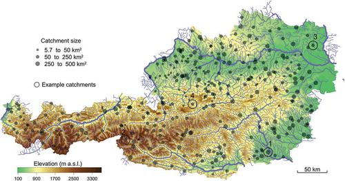
Fig. 3 Distribution of (a) the size of the catchment area, and (b) the flood peak sample sizes in different elevation zones.

Hourly discharge data from the 330 catchments with records in the period 1971–2007 were used. From the discharge data, annual maximum flood peak discharges were derived, resulting in a total of 7163 peaks (i.e. 22 events per catchment, on average). The distribution of the number of peaks per catchment in the different elevation zones is shown in Fig. 3(b). The number of catchments with small samples (10–14 peaks) is similar in each elevation zone (≤10) which would not point to any biases regarding estimation uncertainty. Larger samples (≥20) dominate in the lower elevation zones, up to 1500 m a.s.l. However, for elevations above 1500 m, the portion of larger samples decreases.

METHODS

The dataset used in this paper is based on previous work in the study area (Merz and Blöschl 2003, Merz et al. 2006, Merz and Blöschl 2009, Gaál et al. 2012). While there are several possibilities to identify events and separate direct runoff volumes from the hydrograph (Gonzales et al. 2009), the same methods as in Merz et al. (2006) and Gaál et al. (2012) were used here. In a first step, direct runoff and the baseflow were separated by the digital filter of Chapman and Maxwell (1996). In a second step, the start and the end points of the rainfall–runoff events were identified based on criteria related to direct runoff and the baseflow at the beginning and end of the event. In a final step, a simple rainfall–runoff model, using hourly rainfall and snowmelt inputs, was fitted to the direct hydrograph to estimate the total direct runoff volume. This procedure yields more accurate volume estimates than the direct integration of observed direct runoff hydrograph, as the latter approach will underestimate the volumes since the trailing limb is cut off at the end of the event. Snow processes were accounted for by the soil moisture accounting model of Parajka et al. (2006). Details of the procedure are given in Merz et al. (2006).

The duration of an event is defined as the difference between the times of its end and its beginning, expressed in hours. The coefficient of variation of flood durations is then introduced to characterize the variability of flood events at a given catchment in terms of their durations:

(1)

where σ_Dur and Ave_Dur denote the standard deviation and mean of flood durations, respectively. The coefficient of variation of flood peaks, CV_Q, is defined in a similar way.

For each flood event identified by the above procedure, a flood type was assigned on the basis of the classification of Merz and Blöschl (2003), who classified all annual floods into one of five flood types (long rain floods, short rain floods, flash floods, snowmelt floods and rain-on-snow floods) based on the meteorological situation (spatial extent, intensity and type of precipitation) and the state of the catchment (soil moisture, snow coverage, snowmelt etc.) before and during the individual flood events. In this study, the number of flood processes was reduced to three in order to increase the number of floods per flood type. The merging of flood types was motivated by the low frequency of occurrence of flash floods and snowmelt floods in the original classification of Merz and Blöschl (2003). In this case, due to their small number, it would not be possible to study flash floods and snowmelt floods at the majority of sites. Discarding these two flood types was not an option for us; thus, we decided to merge the original categories into larger ones. The only reasonable option was to merge snow-related flood events (snowmelt floods and rain-on-snow floods) into one category termed ‘snow-related floods’, and those of synoptic origin (long rain and short rain floods) into ‘synoptic floods’. Unfortunately, the category of flash floods had to remain untouched, since the hydrological/climatological/meteorological conditions of their genesis differ significantly from those of the other flood types.

To quantify the strength of association between maximum annual flood discharges and the associated flood volumes of direct runoff, the Spearman rank correlation coefficient ρ between these two variables was estimated for each catchment. The rank correlation coefficient was chosen because (a) it is not sensitive to the magnitude of the extremes, and (b) it may appear as the parameter of copulas in bivariate frequency modelling of flood events. The Spearman rank correlation coefficient assesses how well the relationship between two variables can be described by a monotonic function. It was estimated as:

(2)

where D_i is the difference in ranks between the ith pair of peaks and volumes and n is the number of events per catchment.

To characterize the regularity of occurrence of annual flood maxima within the year, the strength of the flood seasonality was calculated by directional statistics (e.g. Burn 1997) using Equation 6 of Parajka et al. (2009). The strength of seasonality ranges from (uniform flood distribution throughout the year) to (all annual floods occur on the same day of the year).

RESULTS

Catchment controls

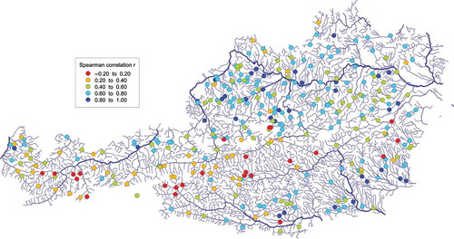
As a first step in the analysis, the spatial distribution of Spearman rank correlation coefficients ρ between flood peaks and volumes is presented in Fig. 4. There is a clear pattern of low ρ along the main ridge of the Alps (Fig. 2) and much higher ρ in the northern and eastern lowlands. Overall, the pattern of ρ is quite complex, as it reflects the joint effect of a wide range of climatological and geological driving factors. However, the geographical distribution of ρ does suggest that one of the most important factors determining the consistency between flood peaks and volumes may be related to snow processes, as these differ by elevation.

Fig. 4 Spatial distribution of Spearman’s correlation coefficient between flood peaks and volumes in Austria.

Spearman’s ρ was then related to selected catchment attributes, beginning with catchment area as the most obvious one (Fig. 5). The colours clearly indicate the increasing correlation coefficient with decreasing elevation: values of ρ ≥ 0.8 mainly occur at elevations below 1000 m a.s.l., and the smallest ρ occur at elevations above 1000 m, although there is a lot of scatter. In Fig. 5, the nested catchments are connected by lines to highlight the scale dependence for the same set of catchments. While, overall, there is little scale dependence, the nested catchments do show a slight trend of increasing consistency between peaks and volumes with increasing catchment area. However, catchments with larger areas tend to lie at lower elevations, so the scale dependence may indicate the effect of spurious correlations with elevation. To identify the controlling attributes in more detail, the linear relationship between Spearman’s ρ and a number of additional catchment attributes is presented in Table 1. This is consistent with the use of linear models (i.e. regressions) in the regionalization of hydrological variables from catchment characteristics. The Pearson correlation coefficient (R²) between ρ and the logarithm of catchment area is null, indicating that indeed the slight tendency of scale dependence in Fig. 5 is not significant. The Pearson correlation coefficient between ρ and mean catchment elevation shows a significant relationship, with R² = 0.35 (for univariate correlation, the minus indicates that they are inversely related). The linear correlations with other catchment attributes are not very large (Table 1). For example, the (univariate) correlations with stream network density and mean catchment slope are R² = 0.12 and 0.25, respectively. Bivariate correlations with mean catchment elevation and other catchment attributes hardly increase the R² beyond the univariate correlation between ρ and mean catchment elevation, indicating that the explanatory power of stream network density and mean catchment slope is through their correlations with mean catchment elevation rather than direct. A rank correlation analysis gives similar magnitudes of the correlation coefficients. Correlations between ρ and other catchment attributes, such as land-use characteristics (percent forest, percent agricultural area) and climatological characteristics (mean summer precipitation, mean winter precipitation), as well as characteristics of geology and soil types (not shown here), give similarly low correlations. This suggests that mean catchment elevation is the main control on Spearman’s ρ that can be identified from the statistical analysis.

Fig. 5 Spearman rank correlation between flood peaks and volumes vs catchment area. Lines connect nested catchments, which are highlighted by larger circles. Colours indicate mean catchment elevation.

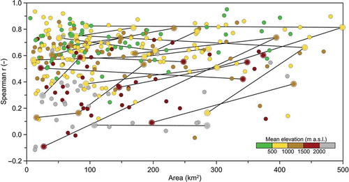
Table 1 Univariate and bivariate linear correlations (adjusted Pearson’s R² in %) of Spearman’s ρ and two catchment attributes. Linear correlations that are significant at the 95% confidence level are in bold. For the univariate correlations (first column), the sign of the correlation coefficient R is indicated. Catchment attributes: log(Area): log of the catchment area; Mean elevation: mean catchment elevation (m a.s.l.); RND: river network density; MAP: mean annual precipitation (mm); Slope: mean topographic slope. For details of the attributes see Merz and Blöschl (2009).

	Univariate	log(Area)	Mean elevation	RND	MAP	Slope
log(Area)	0	–	35	12	1	25
Mean elevation	35^-	35	–	35	36	34
RND	12^+	12	35	–	12	27
MAP	1^+	1	36	12	–	29
Slope	25^-	25	34	27	29	–

To analyse the effect of the temporal variability of flood event characteristics, Fig. 6 presents Spearman’s ρ (colour coded) as a function of the coefficient of variation of the flood durations (CV_Dur, left axis), the coefficient of variation of the flood peaks (CV_Q, right axis) and mean catchment elevation (vertical axis). The linear correlation coefficient between ρ and CV_Q is 0.243 and that between ρ and CV_Dur is –0.377.

Fig. 6 Spearman rank correlation between flood peaks and volumes (colour coded), as a function of the coefficient of variation of flood peaks (CV_Q), the coefficient of variation of flood durations (CV_Dur) and the mean catchment elevation. Duration is defined here as the time difference between beginning and end of the flood event.

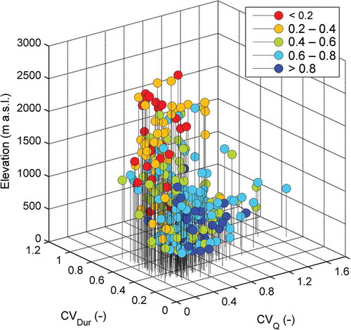
High values of ρ (≥0.6, indicated by blue and cyan in Fig. 6) have a tendency to occur in catchments with low variability of flood durations (lower than the median CV_Dur of 0.45), and high variability of flood peaks (larger than the median CV_Q of 0.53). Low variability of durations may be an indicator of similarity in the flood types. If all annual events in a catchment exhibit similar flood types (and hence durations), one would expect high consistency in the peak–volume relationship. Figure 6 also shows that these tend to be the low-elevation catchments.

The same holds for the opposite end of the ρ spectrum. The catchments with the lowest values of ρ (≤0.4, orange and red in Fig. 6) are associated with high variability of flood durations and low variability of flood peaks. This would be an indicator of the occurrence of a range of different flood types (snow, synoptic floods, flash floods) in a given catchment. The differences in the durations of the floods are the main reason for a weak relationship between peak and volume, which one would expect as the volumes are highly correlated to the product of duration and peak flows. Figure 6 also shows that these tend to be the high-elevation catchments. This means that the catchments with the lowest Spearman’s ρ generally lie at the highest elevations and, as soon as one approaches lower elevations, the consistency between the flood peaks and volumes goes up. The question now is: Which processes, or combination of processes, are responsible for such a pattern of the measure of flood consistency?

It should be noted that, due to the relatively small sample size (10–31 events), there is considerable uncertainty associated with Spearman’s ρ, and this uncertainty increases as ρ approaches zero (Bonett and Wright 2000). For instance, for the sample size n = 23 (the median of all sample sizes) and ρ = 0.613 (the median of all the Spearman correlation coefficients), the estimation uncertainty is σ_ρ = 0.151 (error standard deviation), according to Bonett and Wright (2000). When interpreting the results, these uncertainties need to be kept in mind.

Climate controls

To obtain a first insight into the effect of the flood types, Fig. 7 presents flood peaks and volumes for the entire set of events analysed herein, stratified by the three flood processes: floods of synoptic origin, flash floods and snow-related floods. There are indeed substantial differences between the flood types. The flash floods are associated with the flattest slope of the flood peak–volume relationship, indicating the fastest response. Snow-related floods produce the steepest slope, and the synoptic floods are in between, as one would expect from the results of Gaál et al. (2012). Although only few events have been classified as flash floods (1.8%), this seems to be a robust result.

Fig. 7 Relationship between flood peaks (in mm/h) and flood volumes (in mm) for all flood events analysed herein, stratified by flood process type: synoptic floods (yellow circles), flash floods (cyan triangles) and snow-related floods (magenta asterisks). 95% prediction intervals are shown.

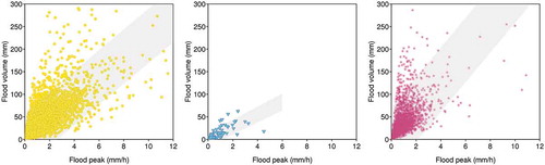
In this paper, the interest lies in the spread of the points around the regression lines: the spread is smallest for flash floods (R² = 0.53), largest for snow-related floods (R² = 0.20), and the synoptic floods are in between (R² = 0.45). Apparently, the shapes of snowmelt floods are the most diverse of all the flood types examined. This is because they include alpine snowmelt floods that may last a week or more.

The findings from Fig. 7 support the notion that there are different flood generation mechanisms and that they are distinguishable in terms of how tight the peak–volume relationships are. It should be noted that Fig. 7 is for all catchments combined, while relationships for individual catchments are analysed below.

Figure 8 shows Spearman’s ρ as a function of climate characteristics (snow-to-precipitation ratio, strength of flood seasonality on the horizontal axes) and flood type probability (colour scale). If, in a given catchment, all floods are synoptic, they are plotted as yellow; if all floods are snow-related they are plotted as magenta; and if all floods are flash floods they are plotted as cyan. Mixed processes are interpolated on an RBG scale, so a catchment with snow-related and synoptic floods would plot orange (magenta+yellow), and a catchment with flash floods and synoptic floods would plot green (cyan+yellow). Mean catchment elevations above 1000 m are plotted as triangles and those below as circles.

Fig. 8 Spearman rank correlation between flood peaks and volumes, as a function of flood type probability (colour), elevation (point type) and climate characteristics (horizontal axes): (a) snow-to-precipitation ratio, (b) strength of flood seasonality, . See text for explanation.

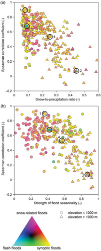
Figure 8(a) indicates that Spearman’s ρ decreases with increasing snow-to-precipitation ratio. Where most of the precipitation falls as rain (small snow-to-precipitation ratio), peaks and volumes tend to be quite consistent, but increasing snowfall tends to reduce the consistency. This is an effect that adds causality to the elevation dependence of ρ in Fig. 6, as the driving processes seem to be related to snowfall rather than elevation itself. Of course, elevation and snow-to-precipitation ratio are highly correlated (R² = 0.83). The fraction of snow-related events (i.e. the ratio of snowmelt and rain-on-snow events to the total number of events at the given site, dark orange) tends to decrease with elevation. At first sight, this is counter-intuitive, but it can be explained by the flood processes in Austria (Merz and Blöschl 2003): at high elevations there are mainly summer floods, driven by synoptic rainfall and some snow-related floods, while at low elevations winter floods with a snow component may be more frequent (Figure 12 in Merz and Blöschl 2003). This suggest that it is not the flood type per se (e.g. snow vs synoptic) that controls the peak–volume dependence, but the nature of the snow-related floods in terms of whether it is a lowland snow flood (which can be quite short), or an alpine snow flood (with typical durations of a week or more). This aspect is analysed in more detail below, for the example catchments.

Fig. 9 Example catchment, Tillmitsch/Lassnitz, in southeastern Austria (area: 480.4 km², mean elevation: 585 m a.s.l.). Hydrographs of maximum annual floods stratified by flood type and colour coded by season. Bottom right: flood volumes colour coded by season.

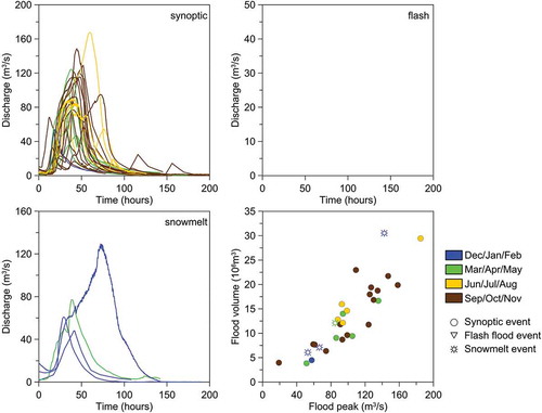
Fig. 10 Example catchment, Hinterbichl/Isel, in southwestern Austria (area: 107.0 km², mean elevation: 2523 m a.s.l.). See Fig. 9 for details.

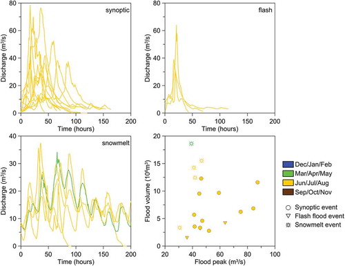
Fig. 11 Example catchment, Bad Pirawarth/Weidenbach, in northeastern Austria (area: 71.0 km², mean elevation: 221 m a.s.l.). See Fig. 9 for details.

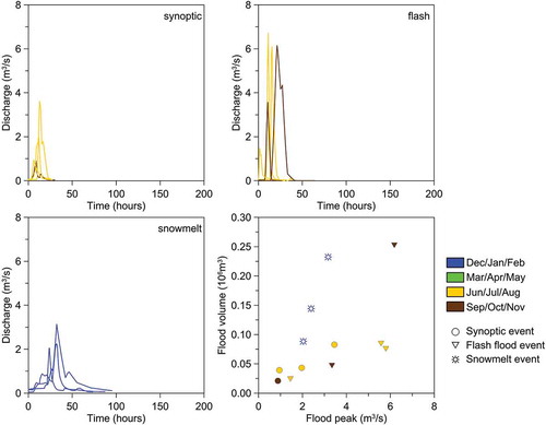
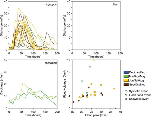
Fig. 12 Example catchment, Kainisch/Ödenseetraun, in central Austria (area: 55.3 km², mean elevation: 1291 m a.s.l.). See Fig. 9 for details.

Figure 8(b) indicates that Spearman’s ρ also decreases with the strength of the flood seasonality. The high Alpine areas have the strongest flood seasonality in Austria, where all the annual floods occur in the summer (Parajka et al. 2010). These are both synoptic floods, some flash floods as well as snow-related floods of long durations. Thus, during a relatively short but wet period of the year, different flood processes may occur in these catchments, resulting in an inconsistent relationship of flood peaks and volumes, and low ρ. Conversely, in lowland catchments, the annual floods may appear at any time of the year, but they are more consistent in terms of peak and volume relationships as their shapes are more similar. Catchments where flash floods play an important role (green in Fig. 8) do exhibit strong seasonality, with the main flood occurrence in summer, but they are lowland catchments, so alpine snowmelt never occurs. Because of this, they give rather high values of Spearman’s ρ.

Example catchments

To analyse the causal factors of the consistency or inconsistency of flood peak–volume relationships in more detail, four example catchments from different regions of Austria were selected. These catchments represent typical climatological settings and hydrological response: lowlands vs mountains, different atmospheric circulation types, wet vs dry rainfall regime, high vs low seasonality of floods, different frequencies of flood types and high vs low Spearman’s ρ. Table 2 gives the main hydrological characteristics of the catchments while their locations are shown in Fig. 1. The flood regimes of the example catchments are presented in Figs 9–12. Each figure shows the direct runoff hydrographs of the maximum annual floods stratified by flood type and colour coded by season. The bottom right panels of these figures show the flood volumes vs flood peaks colour coded by season. Note that in order to make the hydrographs for different flood types and example catchments more comparable, the x-axes of all hydrographs were all plotted up to 200 h.

Table 2 Example catchments for analysing the peak–volume relationships in terms of hydrographs. Spearman’s ρ between peaks and volumes (-) is given in parentheses.

Catchment	Tillmitsch	Hinterbichl	Bad Pirawarth	Kainisch
Stream	Lassnitz	Isel	Weidenbach	Ödenseetraun
Location	SE Austria	SW Austria	NE Austria	Central Austria
Catchment area (km^2)	480.4	107.0	71.0	55.3
Mean catchment elevation (m a.s.l.)	585	2523	221	1291
No. of all flood events	30 (0.90)	18 (0.07)	12 (0.70)	25 (0.53)
No. of synoptic flood events	26 (0.88)	10 (0.35)	4 (1.00)	22 (0.71)
No. of flash flood events	0 (-)	3 (1.00)	5 (0.90)	0 (-)
No. of snow flood events	4 (1.00)	5 (0.30)	3 (1.00)	3 (1.00)
Strength of flood seasonality (-)	0.36	0.87	0.42	0.57
Mean annual precipitation (mm/year)	980	1299	567	1593
Snow-to-precipitation ratio (-)	0.079	0.444	0.091	0.256
Mean event runoff coefficient*	0.33	0.65	0.08	0.64
Median flood time scale (h) ^†	35.9	30.2	6.6	52.4

^* from Merz et al. (2006)

^† from Gaál et al. (2012)

Tillmitsch/Lassnitz

The Tillmitsch catchment on the River Lassnitz (Fig. 9) is located in southeastern Austria, near the Slovenian border. Extreme flooding often occurs due to an influx of moist Mediterranean air in autumn, which is reflected in frequent autumn floods. Nevertheless, floods occur in all seasons, resulting in a low strength of seasonality (0.36). This fact explains the catchment’s position in the top left quadrant of the ρ–seasonality relationship in Fig. 8(b). The peak–volume relationship of this catchment yields a high degree of consistency. Small flood peaks are associated with small flood volumes, large peaks with large volumes and Spearman’s ρ is high (0.90). Floods of synoptic origin dominate (87%), with a few snow-related floods. Because of the low elevations (mean catchment elevation: 585 m a.s.l.), the shapes of the snowmelt hydrographs do not differ much from those of the synoptic floods. Moreover, no flash floods were observed as annual flood maxima. For all these reasons, Spearman’s ρ for all floods is practically identical to that for the dominant synoptic flood types (Table 2) and, consequently, the flood peak–volume relationship shows a high degree of consistency.

Hinterbichl/Isel

The second example catchment represents the exact opposite of the first one. The Hinterbichl catchment on the River Isel is located at high elevations in the Central Alps (mean catchment elevation: 2523 m a.s.l.). Almost all annual floods occur in the summer (Fig. 10), because of the short summer season where both rainfall and snowmelt are possible. The hydrograph shapes show diverse patterns. Most floods are synoptic floods, as in most medium-sized to large catchments in Austria. However, there is a substantial number of snow floods and a few flash floods (Table 2). Figure 10 shows the typical shape of the snowmelt hydrographs from the mountains. The different flood types are associated with different peak–volume relationships, which are apparent in both the hydrographs and the scatter plot in Fig. 10. Flash floods give the smallest volumes, snow-related floods the largest volumes, and the synoptic floods are in between (bottom right panel of Fig. 10). Although both synoptic and snowmelt floods are associated with a rather low Spearman rank correlation (0.35 and 0.30, respectively; Table 2), on the basis of Fig. 10 it is obvious that one could represent the different flood types by different peak–volume relationships. However, if one lumps all flood types together, one obtains a weak dependence between peaks and volumes (ρ = 0.07). This is consistent with the hypothesis illustrated in Fig. 1, i.e. a mix of flood types gives a weak peak–volume dependence.

Bad Pirawarth/Weidenbach

The Bad Pirawarth catchment on the River Weidenbach (mean catchment elevation: 221 m a.s.l.) is typical of the northeastern lowlands of Austria. In this part of the country, floods occur throughout the year. Winter floods are often associated with snow. The meteorological forcing is due to a range of processes including convective storms in summer, as indicated by the slim shape of the flash floods in summer and autumn (Fig. 11). Due to the dominance of summer and autumn events, the regularity of flood seasonality is rather small (0.42). Bad Pirawarth is one of the catchments with the largest frequency of flash floods in the current database (5 out of 12). Therefore, even though the other two flood types also appear in the sample, with a similar ratio (4 synoptic floods and 3 snowmelt floods), we can consider Bad Pirawarth as being representative of catchments that have mixed flood types with a slight dominance of flash floods. The Spearman correlation coefficients for the individual flood types are all high (Table 2). Even though the snow-related floods do show greater volumes than the flash floods, the difference is not very big, so the measure of overall peak–volume consistency is rather high (ρ = 0.70). This example nicely illustrates the differences between snow-related floods in the lowlands (Fig. 11) and snow-related floods in the Alpine areas (Fig. 10). Rather than the flood type per se, it is the elevation setting that exerts a major control on the volume characteristics of the floods.

Kainisch/Ödenseetraun

The last of the example catchments, Kainisch, is located in a karstic area along the northern slopes of the Alpine range (mean catchment elevation: 1291 m a.s.l.). Floods mainly occur in the summer and autumn (Fig. 12). The flood regime is dominated by synoptic floods (88%), with a few snow-related floods (12%) but no flash floods. The latter is because of the slow catchment response due to the effect of karst. Since synoptic floods dominate (ρ = 0.71, Table 2), the hydrograph patterns are similar to those of Hinterbichl (Fig. 9). However, the snow-related floods in Kainisch show less pronounced daily fluctuations than in Hinterbichl due to the lower elevations. Similar to Hinterbichl and Bad Pirawarth, the snow-related floods have larger volumes than the other floods. The difference is less pronounced than in the high-elevation Hinterbichl catchment, but more pronounced than in the low-elevation Bad Pirawarth catchment, and Spearman’s ρ is in between (ρ = 0.53). This explains the strong control of elevation demonstrated in most of this paper. Furthermore, the Kainisch catchment is a nice illustration of the hypothesis shown in Fig. 1: mixing two flood processes, each with high consistency between flood peaks and volumes, results in lower overall consistency between them.

DISCUSSION

General remarks

The purpose of this study was to analyse the dependence between flood peaks and the corresponding flood volumes in a regional context, and to understand the causal factors controlling this dependence. The analysis was performed for annual maximum floods, using Austria as a case study area. While Gaál et al. (2012) analysed the average dependence between peaks and volumes based on flood time scales, this study was concerned with the degree of consistency between peaks and volumes and their controls.

To express the strength of association between flood peaks and flood volumes, the Spearman rank correlation coefficient was estimated for each site. In the majority of analyses, Spearman’s ρ was estimated on the basis of all events at the given site, regardless of their genesis, since, in general, flood types are not commonly available in studies of flood peak–volume relationships.

Note, when interpreting the results, it needs to be kept in mind that, due to the relatively small sample sizes (10–31 events), there is uncertainty associated with Spearman’s ρ. It should also be noted that this paper does not focus on statistical models of the dependence structure in a multivariate relationship (e.g. appropriateness of a specific copula family), but on whether flood peak–volume relationships can be typified by methods of comparative hydrology, or, in other words, whether it is possible to discriminate flood types and the strength (Spearman’s ρ) and shape (visual comparison) of the association between the two variables spatially.

The possible non-stationarity of the runoff regime in the Alpine region (as discussed in detail in Castellarin and Pistocchi 2012) may be one of the further important factors that could influence the results; nevertheless, analysis of the effects of land-use and climate change on the hydrological regime was beyond the scope of this study.

Climate vs catchment controls

The results suggest that the factors controlling the dependence are mainly related to climate rather than catchment characteristics. This would be expected, as the interest is in the variability between events. Catchment characteristics are essentially stationary at the time scales analysed, so the temporal variability mainly comes from the climate forcing. The results also suggest that snowmelt floods tend to be more diverse than synoptic floods and flash floods in terms of their durations, which translates into a weaker dependence of the peak–volume relationship than for the other two flood types. This is consistent with the findings of Renard and Lang (2007) in the French Ubaye River. They noted a “lack of shape invariance for snow related events”, as moderate rainfalls can be superimposed on high baseflow produced by snowmelt, thus leading to a great variety of hydrograph shapes for the same river. When they analysed only rain-fed floods, the hydrograph shapes were much more consistent.

The role of catchment elevation

While the analysis of the peak–volume dependence by flood type was very insightful, an important finding of this study is the paramount role of catchment elevation in that dependence. The lowest Spearman rank correlation coefficients between peaks and volumes occurred in the high alpine catchments, with typical values around 0.2. The highest Spearman rank correlation coefficients occurred in the lowlands, with typical values around 0.8. From a process perspective, the main difference between alpine and lowland floods is the role of snow and the characteristics of snow-related floods. This is supported by analysis of the Spearman rank correlation coefficients with respect to snow-to-precipitation ratio and strength of flood seasonality. The correlations between peak and volume consistently decrease with increasing snow-to-precipitation ratio and strength of flood seasonality. These two variables are closely related to elevation through temperature and therefore snow processes.

Mountain catchments

In the mountain catchments, such as Hinterbichl, the flood season is relatively short, mainly in summer, but a diverse set of flood types may occur, including long-duration snowmelt floods, synoptic floods and flash floods. Because of this mix of different flood types, the dependence between flood peaks and volumes is weak. If only a limited number of flood types occurs, e.g. only synoptic floods, this will increase the strength of association between peaks and volumes, as the flood durations are more consistent. This finding is consistent with the reasoning outlined in the introduction (Fig. 1). The important point is that the mountain type snowmelt, which exhibits long durations and large flood volumes, when combined with synoptic events and flash floods, will result in a low degree of consistency between flood peaks and volumes.

Lowland catchments

In the lowlands, the flood durations vary less. This is because of a number of factors. Most importantly, long-duration snowmelt floods are absent. Snow-related floods, usually rain on snow events, are not too different from other flood types in terms of their volumes. Second, the events that produce the maximum annual floods are those for which the storm duration is close to the concentration time of the catchment, because the catchment-response time scales filter the distribution of all storms to produce the distribution of flood-producing storms. Third, the co-evolution of climate, landform, soils and vegetation may contribute to a more consistent flood response between events. At the time scale of decades, the flow paths as well as soil moisture affect both erosion during floods and soil evolution (modulated by differences in geology), while soil depth and permeability affect flow paths and therefore the flood response at the event scale. Even at the landscape evolution time scale, there are further interactions. Gaál et al. (2012) showed catchments whose form has adapted to the flashiness of floods by producing efficient drainage networks, which, in turn, enhance the flashiness of the flood response. In other catchments, tortuous drainage networks have evolved, which, in turn, retard the flood response and impede the evolution of an efficient drainage network. This means that, in the absence of long-duration snowmelt floods, the flood peak–volume relationships will be more consistent.

CONCLUSIONS

The main conclusion of this study is that a mix of different flood types reduces the consistency between flood peaks and volumes. However, this particularly applies to catchments with long-duration snowmelt floods. To fully capture the effect on the dependence between peaks and volumes, the nature of snow-related floods—long-duration snowmelt floods in mountains vs shorter snow-related floods in lowlands—needs to be ascertained. In lowland catchments, peaks and volumes tend to be more consistent because of the filtering of the distribution of all storms by the catchment response time to produce the distribution of flood producing storms, and the co-evolution of climate, landform and soils.

The findings reported in this paper have implications for the choice of statistical dependence structure between flood peaks and volumes. For most cases of practical interest there are not enough data to reliably fit copula models of peaks and volumes for large return periods. This is because of the higher dimensionality of bivariate models compared to univariate models. While copula models, often, only involve a single parameter (e.g. Genest and Favre 2007, Chowdhary et al. 2011), the choice of copula function then plays a role in deciding the shape of the dependence. In choosing the copula, the causal factors identified in this paper could be used as a priori information. This applies to static characteristics such as mean catchment elevation, as well as more dynamic characteristics such as snow-to-precipitation ratio, strength of the flood seasonality and presence or absence of long-duration snowmelt floods. This a priori information could be accounted for in a framework of a flood frequency hydrology. One possibility is to include the information through process reasoning along the lines given in Merz and Blöschl (2008a, 2008b). Alternatively, a more rigorous Bayesian analysis could be used, as illustrated by Viglione et al. (2013) for the case of flood peaks. Overall, the aim is to reduce the estimation uncertainty by including information that goes beyond the systematic dataset of flood peak discharges and the associated flood volumes.

It needs to be emphasised that this study does not focus on the statistical properties of the dependence, but on whether flood peak–volume relationships can be typified by comparative hydrology; in other words, whether it is possible to relate flood types and the strength and shape of the association between two variables associated with these spatially. The results of this study indicate that there are potential differences, and these may be the subject of statistical modelling in upcoming studies.

There are opportunities for future work to extend the analyses of the present study. The dataset of this study consists of maximum annual floods, so the number of events available for each catchment was equal to the record length in years, which ranged from 10 to 37. If one performs bivariate analyses of peak and volume, a large sample size is even more important than for univariate analyses. Stratifying the data by flood type further reduces the sample size. It would therefore be interesting to extend the present work using peak-over-threshold data to increase the sample size, or to use all the independent rainfall–runoff events that it is possible to identify in the given catchment. Large data samples for multivariate analyses could also be obtained by rainfall–runoff modelling and derived flood frequency analysis. Also, there were relatively few flash floods in the dataset because of the relatively large catchments (median catchment size: approx. 100 km²). Opportunities exist to add non-systematic data on flash floods (Gaume et al. 2009, 2010, Borga et al. 2011, Pekárová et al. 2012),  although the statistical characterizations may not be straightforward. Finally, estimating flood event volumes is always a problem, in particular for long-duration snowmelt floods, as there is no single best method, and more research is needed here. Perhaps more importantly, considering double events would be a useful extension, in particular from a practical perspective (Blöschl et al. 2013b). These analyses could be performed in a comparative hydrology framework (Blöschl et al. 2013a) to make the results applicable to a wide range of catchment conditions.

Disclosure statement

No potential conflict of interest was reported by the authors.

Acknowledgements

We are very grateful to the two reviewers, M. Thyer and F. Serinaldi, and to the editor, Z.W. Kundzewicz, whose comments greatly improved the quality of the initial manuscript.

Additional information

Funding

We would like to thank the Austrian Academy of Sciences (International Strategy for Disaster Reduction Programme, IWHRE2008, 2008–2013), the ERC (Advanced Grant on Flood Change) and the FWF (project no. P 23723-N21) for financial support. This research was also supported by the Slovak Research and Development Agency (under contract no. APVV 0496–10), the Slovak Grant Agency VEGA (project no. 1/0776/13) and the IMPALA (FP7-PEOPLE-2011-IEF-301953) project of the Marie Curie Intra European Fellowship within the 7th European Community Framework Programme.

REFERENCES

- Bačová-Mitková, V. and Halmová, D., 2014. Joint modeling of flood peak discharges, volume and duration: a case study of the Danube river in Bratislava. Journal of Hydrology and Hydromechanics. doi:10.2478/johh–2014–0026
- Blöschl, G., 2006. Hydrologic synthesis: across processes, places, and scales. Water Resources Research, 42, W03S02. doi:10.1029/2005WR004319
- Blöschl, G. et al., eds., 2013a. Runoff prediction in ungauged basins—synthesis across processes, places and scales. Cambridge: Cambridge University Press.
- Blöschl, G., et al., 2013b. The June 2013 flood in the Upper Danube basin and comparisons with the 2002, 1954 and 1899 floods. Hydrology and Earth System Sciences, 17, 5197–5212. doi:10.5194/hess-17-5197–2013
- Blöschl, G. and Merz, R., 2009. Landform –hydrology feedbacks. In: J.-C. Otto and R. Dikau, eds. Landform –structure, evolution, process control, Lecture notes in Earth Sciences. 115. Heidelberg: Springer Verlag, 117–126. doi:10.1007/978-3-540-75761-0_8
- Bonett, D.G. and Wright, T.A., 2000. Sample size requirements for estimating Pearson, Kendall and Spearman correlations. Psychometrika, 65 (1), 23–28. doi:10.1007/BF02294183
- Borga, M., et al., 2011. Flash flood forecasting, warning and risk management: the HYDRATE project. Environmental Science & Policy, 14, 834–844. doi:10.1016/j.envsci.2011.05.017
- Burn, D.H., 1997. Catchment similarity for regional flood frequency analysis using seasonality measures. Journal of Hydrology, 202 (1–4), 212–230. doi:10.1016/S0022–1694(97)00068–1
- Castellarin, A. and Pistocchi, A., 2012. An analysis of change in alpine annual maximum discharges: implications for the selection of design discharges. Hydrological Processes, 26, 1517–1526. doi:10.1002/hyp.8249
- Chapman, T.G. and Maxwell, A.I., 1996. Baseflow separation—comparison of numerical methods with tracer experiments. In: 23rd Hydrology and Water Resources Symposium: Water and the Environment. Barton, ACT: Inst. of Eng., National Conference Publ., 96/05, 539–545.
- Chen, L., et al., 2010. A new seasonal design flood method based on bivariate joint distribution of flood magnitude and date of occurrence. Hydrological Sciences Journal, 55 (8), 1264–1280. doi:10.1080/02626667.2010.520564
- Chowdhary, H., Escobar, L.A., and Singh, V.P., 2011. Identification of suitable copulas for bivariate frequency analysis of flood peak and flood volume data. Hydrology Research, 42 (2–3), 193. doi:10.2166/nh.2011.065
- Corradini, C., Melone, F., and Singh, V.P., 1995. Some remarks on the use of GIUH in the hydrological practice. Nordic Hydrology, 26, 297–312. doi:10.2166/nh.1995.017
- De Michele, C., et al., 2005. Bivariate statistical approach to check adequacy of dam spillway. Journal of Hydrologic Engineering, 10 (1), 50–57. doi:10.1061/(ASCE)1084-0699(2005)10:1(50)
- Dooge, J.C.I., 2005. Bringing it all together. Hydrology and Earth System Sciences, 9 (1/2), 3–14. doi:10.5194/hess-9-3–2005
- Falkenmark, M. and Chapman, T.C., 1989. Comparative hydrology: an ecological approach to land and water resources. Paris: UNESCO.
- Fang, X., et al., 2005. Literature review on timing parameters for hydrographs. Report 0-4696-1, Department of Civil Engineering, College of Engineering, Lamar University, Beaumont, Texas.
- Favre, A.-C., et al., 2004. Multivariate hydrological frequency analysis using copulas. Water Resources Research, 40, W01101. doi:10.1029/2003WR002456
- Folmar, N.D., Miller, A.C., and Woodward, D.E., 2007. History and development of the NRCS lag time equation. Journal of the American Water Resources Association, 43 (3), 829–838. doi:10.1111/j.1752-1688.2007.00066.x
- Gaál, L., et al., 2012. Flood timescales: understanding the interplay of climate and catchment processes through comparative hydrology. Water Resources Research, 48 (4), W04511. doi:10.1029/2011WR011509
- Gaume, E., et al., 2009. A compilation of data on European flash floods. Journal of Hydrology, 367 (1–2), 70–78. doi:10.1016/j.jhydrol.2008.12.028
- Gaume, E., et al., 2010. Bayesian MCMC approach to regional flood frequency analyses involving extraordinary flood events at ungauged sites. Journal of Hydrology, 394 (1–2), 101–117. doi:10.1016/j.jhydrol.2010.01.008
- Genest, C. and Favre, A.-C., 2007. Everything you always wanted to know about copula modeling but were afraid to ask. Journal of Hydrologic Engineering, 12 (4), 347–368. doi:10.1061/(ASCE)1084-0699(2007)12:4(347)
- Goel, N.K., Seth, S.M., and Chandra, S., 1998. Multivariate modeling of flood flows. Journal of Hydraulic Engineering, 124 (2), 146–155. doi:10.1061/(ASCE)0733-9429(1998)124:2(146)
- Gonzales, A.L., et al., 2009. Comparison of different base flow separation methods in a lowland catchment. Hydrology and Earth System Sciences, 13, 2055–2068. doi:10.5194/hess-13-2055–2009
- Gräler, B., et al., 2013. Multivariate return periods in hydrology: a critical and practical review focusing on synthetic design hydrograph estimation. Hydrology and Earth System Sciences, 17, 1281–1296. doi:10.5194/hess-17-1281-2013
- Grimaldi, S. and Serinaldi, F., 2006. Asymmetric copula in multivariate flood frequency analysis. Advances in Water Resources, 29 (8), 1155–1167. doi:10.1016/j.advwatres.2005.09.005
- Harlina, J.M., 1984. Watershed morphometry and time to hydrograph peak. Journal of Hydrology, 67, 141–154. doi:10.1016/0022–1694(84)90238–5
- Hirschboeck, K.K., Ely, L., and Maddox, R.A., 2000. Hydroclimatology of meteorologic floods. In: E. Wohl, ed. Inland flood hazards: human, riparian and aquatic communities. New York: Cambridge University Press, 39–72.
- McCuen, R.H., Wong, S.L., and Rawls, W.J., 1984. Estimating urban time of concentration. Journal of Hydraulic Engineering, 110 (7), 887–904. doi:10.1061/(ASCE)0733-9429(1984)110:7(887)
- Melone, F., Corradini, C., and Singh, V.P., 2002. Lag prediction in ungauged basins: an investigation through actual data of the upper Tiber River valley. Hydrological Processes, 16 (5), 1085–1094. doi:10.1002/hyp.313
- Merz, R. and Blöschl, G., 2003. A process typology of regional floods. Water Resources Research, 39 (12), 1340. doi:10.1029/2002WR001952
- Merz, R. and Blöschl, G., 2008a. Flood frequency hydrology: 1. Temporal, spatial, and causal expansion of information. Water Resources Research, 44 (8), W08432. doi:10.1029/2007WR006744
- Merz, R. and Blöschl, G., 2008b. Flood frequency hydrology: 2. Combining data evidence. Water Resources Research, 44 (8), W08433. doi:10.1029/2007WR006745
- Merz, R. and Blöschl, G., 2009. A regional analysis of event runoff coefficients with respect to climate and catchment characteristics in Austria. Water Resources Research, 45 (1), W01415. doi:10.1029/2008WR007163
- Merz, R., Blöschl, G., and Parajka, J., 2006. Spatio-temporal variability of event runoff coefficients. Journal of Hydrology, 331 (3–4), 591–604. doi:10.1016/j.jhydrol.2006.06.008
- Parajka, J., et al., 2006. Assimilating scatterometer soil moisture data into conceptual hydrologic models at the regional scale. Hydrology and Earth System Sciences, 10, 353–368. doi:10.5194/hess-10-353–2006
- Parajka, J., et al., 2009. Comparative analysis of the seasonality of hydrological characteristics in Slovakia and Austria. Hydrological Sciences Journal, 54 (3), 456–473. doi:10.1623/hysj.54.3.456
- Parajka, J., et al., 2010. Seasonal characteristics of flood regimes across the Alpine–Carpathian range. Journal of Hydrology, 394 (1–2), 78–89. doi:10.1016/j.jhydrol.2010.05.015
- Pavelková, H., Dohnal, M., and Vogel, T., 2012. Hillslope runoff generation - comparing different modeling approaches. Journal of Hydrology and Hydromechanics, 60 (2), 73–86. doi:10.2478/v10098-012-0007-2
- Pekárová, P., et al., 2012. Estimating flash flood peak discharge in Gidra and Parná Basin: case study for the 7–8 June 2011 flood. Journal of Hydrology and Hydromechanics, 60 (3), 145–216. doi:10.2478/v10098-012-0018–z
- Rao, A.R., Delleur, J.W., and Sarama, P.B.S., 1972. Conceptual hydrologic models for urbanizing basins. Journal of Hydraulic Division ASCE, 98 (HY7), 1205–1220.
- Renard, B. and Lang, M., 2007. Use of a Gaussian copula for multivariate extreme value analysis: some case studies in hydrology. Advances in Water Resources, 30 (4), 897–912. doi:10.1016/j.advwatres.2006.08.001
- Requena, A.I., Mediero, L., and Garrote, L., 2013. Bivariate return period based on copulas for hydrologic dam design: comparison of theoretical and empirical approach. Hydrology and Earth System Sciences Discussions, 10, 557–596. doi:10.5194/hessd-10-557-2013
- Sackl, B. and Bergmann, H., 1987. A bivariate flood model and its application. In: V.P. Singh, ed. Hydrologic frequency modelling. Proceedings of the international symposium on flood frequency and risk analyses. New York: Springer Science & Business Media, 571–582.
- Salvadori, G., De Michele, C., and Durante, F., 2011. On the return period and design in a multivariate framework. Hydrology and Earth System Sciences, 15, 3293–3305. doi:10.5194/hess-15-3293–2011
- Serinaldi, F. and Kilsby, C.G., 2013. The intrinsic dependence structure of peak, volume, duration and average intensity of hyetographs and hydrographs. Water Resources Research, 49 (6), 3423–3442. doi:10.1002/wrcr.20221
- Sheridan, J.M., 1994. Hydrograph time parameters for flatland watersheds. Transactions of the ASAE, 37 (1), 103–113. doi:10.13031/2013.28059
- Shiau, J.T., 2003. Return period of bivariate distributed extreme hydrological events. Stochastic Environmental Research and Risk Assessment (SERRA), 17, 42–57. doi:10.1007/s00477-003-0125–9
- Viglione, A., et al., 2010a. Quantifying space-time dynamics of flood event types. Journal of Hydrology, 394 (1–2), 213–229. doi:10.1016/j.jhydrol.2010.05.041
- Viglione, A., et al., 2010b. Generalised synthesis of space–time variability in flood response: an analytical framework. Journal of Hydrology, 394 (1–2), 198–212. doi:10.1016/j.jhydrol.2010.05.047
- Viglione, A., et al., 2013. Flood frequency hydrology: 3. A Bayesian analysis. Water Resources Research, 49 (2), 675–692. doi:10.1029/2011WR010782
- Viglione, A. and Blöschl, G., 2009. On the role of storm duration in the mapping of rainfall to flood return periods. Hydrology and Earth System Sciences, 13 (2), 205–216. doi:10.5194/hess-13-205–2009
- Yue, S., et al., 2002. Approach for describing statistical properties of flood hydrograph. Journal of Hydrologic Engineering, 7 (2), 147–153. doi:10.1061/(ASCE)1084-0699(2002)7:2(147)
- Zegpi, M. and Fernández, B., 2010. Hydrological model for urban catchments—analytical development using copulas and numerical solution. Hydrological Sciences Journal, 55 (7), 1123–1136. doi:10.1080/02626667.2010.512466