Urban flood hazard mapping using change detection on wetness transformed images

ABSTRACT

The present study demonstrates the use of a new approach for delineating the accurate flood hazard footprint in the urban regions. The methodology involves transformation of Landsat Thematic Mapper (TM) imagery to a three-dimensional feature space, i.e. brightness, wetness and greenness, then a change detection technique is used to identify the areas affected by the flood. Efficient thresholding of the normalized difference image generated during change detection has shown promising results in identifying the flood extents which include standing water due to flood, sediment-laden water and wetness caused by the flood. Prior to wetness transformations, dark object subtraction has been used in lower wavelengths to avoid errors due to scattering in urban areas. The study shows promising results in eliminating most of the problems associated with urban flooding, such as misclassification due to presence of asphalt, scattering in lower wavelengths and delineating mud surges. The present methodology was tested on the 2010 Memphis flood event and validated on Queensland floods in 2011. The comparative analysis was carried out with the widely-used technique of delineating flood extents using thresholding of near infrared imagery. The comparison demonstrated that the present approach is more robust towards the error of omission in flood mapping. Moreover, the present approach involves less manual effort and is simpler to use.

Editor Z.W. Kundzewicz; Associate editor A. Viglione

KEYWORDS:

• flood hazard foot print
• change detection
• wetness transformation
• urban flooding
• dark object subtraction
• scattering
• normalized difference image

Introduction

General

Flood is a relatively high flow of water that overtops the natural and artificial banks in any of the reaches of a stream. When banks are overtopped, water spreads over the flood plain and generally causes problem for inhabitants, crops and vegetation. During extreme flood events it is important to determine quickly the extent of flooding and land use under water (Wang 2004). Flood mapping can be applied to develop a comprehensive relief effort immediately after flooding. There are varieties of issues and uncertainties involved in flood mapping. Remote sensing data has been widely used for flood mapping in the past (Imhoff et al. 1987, Islam and Sado 2002, Jain et al. 2006). This study demonstrates the use of change detection on wetness transformed images for mapping flooding in urban regions.

Challenges

Delineating the flood hazard footprint in urban regions with remotely-sensed imagery is not limited to water extraction. Flood brings in much sludge and sediment-laden water. Moreover, if the satellite image is acquired several days after a flood event, the floodwater will have receded causing the inundated areas to not be delineated accurately using satellite imagery. Water is characterized by low reflectance in the near infrared region of the spectrum (TM4) and comparatively high reflectance in short wavelengths (TM1 and TM2) as shown in Fig. 1. So clear water in ideal situations can be delineated using water indices like the normalized difference water index (NDWI), thresholding on TM band 4, unsupervised classifications (Ridler and Calvard 1978), etc. But in urban regions, asphalt and roof tops have similar characteristics in the near infrared similar to water resulting in erroneous water delineation (Wang et al. 2002).

Figure 1. Spectral reflectance of vegetation, soil and water.

Rayleigh scattering in short wavelength regions also leads to misclassification in urban areas. Moreover, none of the above mentioned methods can successfully delineate wet soil and sediment-laden water which usually represent the flood if itis marked by muddy water or the satellite image is acquired after several days of the flooding.

Wetness transformations

Kauth and Thomas (1976) produced an orthogonal transformation of the original Landsat MSS data to a new four-dimensional feature space. It created four new axes: the soil brightness index (B), greenness vegetation index (G), yellow stuff index (Y) and non-such index (N). The names of the axes refer to the characteristics which they tend to measure. The coefficients in the following formulae (equations (1)−(4)) are from Kauth et al. (1979):

(1)

(2)

(3)

(4)

Crist (1985), using similar grounds, derived the visible, near infrared and middle infrared coefficients for transforming Landsat TM imagery into brightness (B), greenness (G) and wetness (W) variables:

(5)

(6)

(7)

The feature space thus formed is depicted in Fig. 2. The transition between the vegetation and soil plane happens between the two planes shown in Fig. 2.

Figure 2. Feature space generated after transformation.

The derived wetness image made special use of the middle infrared bands (TM5 and TM7) and showed the potential to identify moisture content after several days of the flood event, along with the sludge and mud brought in by the flood to urban areas. This transformation is a global index. Theoretically, it may be used anywhere in the world to disaggregate the amount of soil brightness, vegetation and wetness.

Change detection

Change detection is the process of identifying differences in the state of an object or phenomenon by observing it at different times (Singh 1989). Timely and accurate change detection of Earth’s surface features provides the foundation for a better understanding of the relationships and interactions between human and natural phenomena for managing and using the resources appropriately. In general, change detection involves the application of multi-temporal datasets to quantitatively analyse the temporal effects of the phenomenon. Several methods for carrying out change detection are popular in the literature. These can be algebraic, such as differencing and rationing, transformations, such as principal components analysis (PCA).

Image differencing is one of the most used techniques of change detection. The differenced images can be visualized as percent change images, simple difference or normalized difference images. The latter has computational advantages and reduces the associated change to a magnitude of 0 to 1 on either side of the number line (positive change or negative change).

Objective

The study aims to present an approach for mapping the complete hazard footprint due to a flood event using change detection on wetness transformed images. The footprint here refers to delineating clear water, sediment-laden water and wet soil which are indicators of flood, especially during urban flood and on late acquired imagery. The study also aims at reducing all the errors and shortcomings associated with flooding in urban regions, such as misclassification due to asphalt, scattering of short wavelengths where water has a prominent signature and identifying the wet and moist areas, to aid in flood analysis after a flood event, with a late acquired image.

Study area and flood event

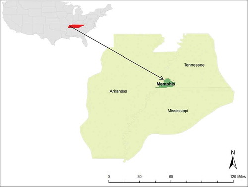
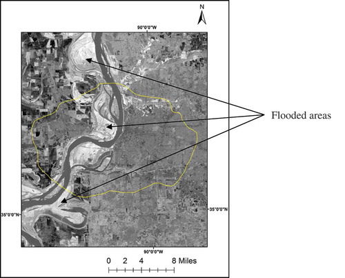
The Mississippi flood of April–May 2011 in the Memphis region was used for the study. The Mississippi River Basin is the third largest in the world, after the Amazon and Congo. Managing floods along the river has challenged engineers for more than a century. The Mississippi River reached 47.87 feet (14.59 m) in Memphis, Tennessee, on 10 May 2011, according to the Advanced Hydrological Prediction Service (AHPS) of the US National Weather Service. It was the highest water level for Memphis since 1937, when the river reached 48.7 feet (14.8 m). In May 2011, muddy water pushed over the Mississippi’s banks on both the east and west sides of the normal river channel. Flood waters spanned the distance between Memphis and West Memphis, and also filled a flood plain extending to an industrial park northwest of Treasure Island. Figure 3 shows the Landsat true colour composite imagery depicting flooding in the Memphis region (Fig. 4) during the 2011 Mississippi flood.

Figure 3. Mississippi flooding as seen from Landsat pre- (left) and post-event (right).

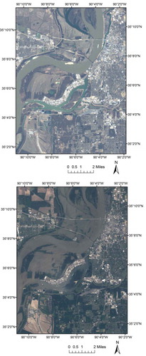
Figure 4. Study area for Memphis floods.

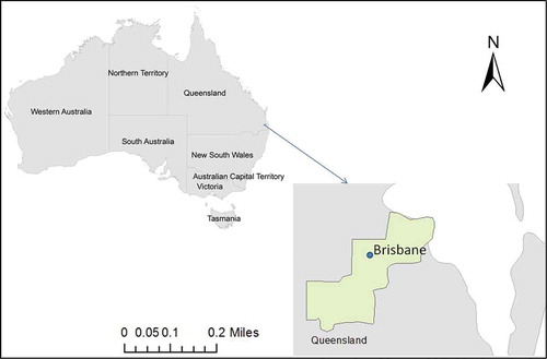
For the validation of the present methodology, the Queensland, Australia, flood event of January 2011 has been taken. This event is another perfect example of a flood event in an urban region. The event was triggered due to a heavy rainfall caused by tropical cyclone Tasha. Due to this major event almost three quarters of Queensland was declared a disaster zone. On 11 January, the Brisbane River broke its banks, leading to evacuations from the commercial business district areas of Brisbane city and towns nearby. Figure 5 shows the area studied for this event, which includes Brisbane city and surrounding towns.

Figure 5. Study area for Queensland floods.

Data used

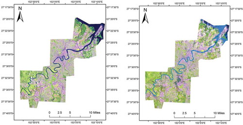
Landsat 5 TM data was used for flood mapping. For the change detection, both pre- and post-flood event imagery were utilized. Table 1 summarizes the acquisition dates of the satellite images used for the Memphis and Queensland flood events. The Thematic Mapper (TM) onboard the Landsat 5 satellite is a medium resolution imaging sensor. TM imagery consists of six reflective and one thermal band. The technical specifications of TM are listed in Table 2. The Linear Imaging Self Scanner (LISS) onboard the Resourcesat-1 satellite and the Advanced Spaceborne Thermal Emission and Reflection Radiometer (ASTER) onboard the Terra satellite measure similar variables to TM with slightly different spatial resolution. Landsat 5 was officially decommissioned on 5 June 2013. The mission was superseded by Landsat 8 launched on 11 February 2013. Figures 6 and 7 show the pre- and post-event TM images of the study areas in false colour composite of TM bands 5, 4 and 3. Water can be seen in various shades of blue.

Table 1. Dates of image acquisition for flood events.

	Memphis	Queensland
Sensor	Thematic Mapper (TM)	Thematic Mapper (TM)
Pre-event image date	4 March 2011	15 December 2011
Post-event image date	10 May 2011	16 January 2011

Table 2. Landsat 5 TM specifications.

	Landsat 5 TM
Launch	1 March 1984
Altitude	705 km
Revisit time	16 days
Spatial resolution	30 m (reflective) 120 m (thermal)
Spectral bands	1: Blue (0.45–0.52 µm)
	2: Green (0.52–0.60 µm)
	3: Red (0.63–0.69 µm)
	4: Near infrared (0.76–0.90 µm)
	5: Short wave infrared (1.55–1.75 µm)
	6: Thermal (10.40–12.50 µm)
	7: Mid infrared (2.08–2.35 µm)
Scene size	184 × 185.2 km

Figure 6. Landsat TM images of 4 March 2011 (left), and 10 May 2011 (right).

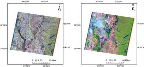
Figure 7. Landsat TM images of 16 December 2010 (left), and 15 January 2011 (right).

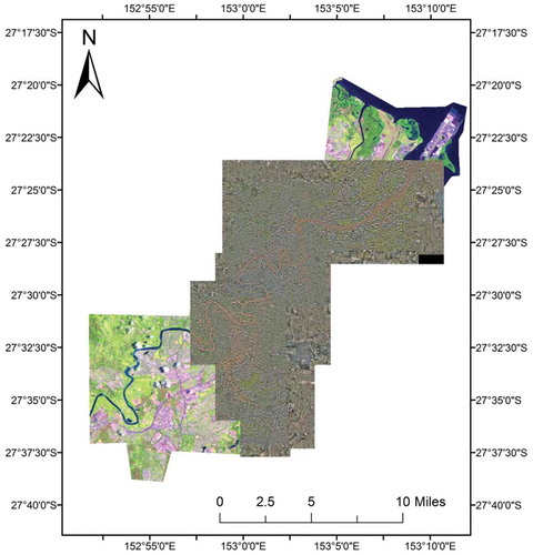
For validation purposes, aerial images captured by NearMap were used. These images were captured on 13 and 14 January, 2011. They have a high spatial resolution of 0.3 m and have standard red, blue and green bands. Figure 8 shows the coverage of the aerial images with respect to the Landsat image.

Figure 8. Coverage of NearMap aerial images with respect to Landsat imagery for Queensland flood.

Methodology

Figure 9 depicts the methodology adopted to extract the flood hazard footprint. The first step is the conversion of DN values to physically meaningful quantities, i.e. reflectance. In the second step, dark object subtraction was applied to the images to reduce the effect of Rayleigh scattering in lower wavelengths (Crippen 1988). Rayleigh scattering is the most dominant atmospheric effect in Landsat TM; it has an additive effect on the image which can be effectively compensated by using dark object subtraction (Song et al. 2001). In this process, the lowest value in the band is subtracted from the whole band, assuming a ‘dark object’ in the image which has zero reflectance. Due to Rayleigh scattering, dark objects in the image are not absolutely dark and have a value above zero (Chavez 1988). The values above zero are assumed to have resulted because of scattering. This methodology has been used previously for compensating scattering in mountainous terrains (Frey et al. 2010). In the present study this method was tested to reduce the scattering effects in urban regions.

Figure 9. Methodology.

In the next step, wetness transformation was applied to the two images using equations (5)–(7). The wetness transformed images are shown in Fig. 10. The bright portions of the image represent water and wetted areas, while the parts with darker tones represent low moisture regions of the area. As can be seen from Fig. 10, the post-event image is brighter in most areas due to flood and rain.

Figure 10. Pre-event wetness transformed image (left), and post-event wetness transformed image (right).

After obtaining the wetness transformed images, change detection was carried out by generating a normalized difference change image. In this image, changes from pre- to post-event images are present in the range from –1 to 1 (Fig. 11). Normalizing the change values makes the data easy and simple to analyse. Higher tones depict greater change. Finally the thresholding was applied to the normalized difference change image to obtain the flood hazard footprint.

Figure 11. Normalized difference change image.

To validate this methodology, the technique has been tested on the Queensland flood event of 5 May, 2011. For this event, high resolution (0.3 m) aerial images were provided by the Near Map agency. The aerial imagery consisted of the three standard bands, red, green and blue. For the comparative analysis of the proposed methodology with the existing flood mapping methodologies, flood extents were also delineated by thresholding of TM4. The Landsat near-infrared band (TM4) is generally used for flood mapping and water body detection due to the low reflectance of water (Qi et al. 2009). Although TM band 4 gives good representation of water compared to other visible bands, but there is always confusion with urban areas, hill shadows and pasture paddocks (Frazier and Page 2000). It has been found that TM band 7 can be used to distinguish asphalt features from water and can be used as an additional band to demarcate asphalt features from water. The major steps in this approach are:

• Identification of water and non-water areas in pre- and post-event images by thresholding of the TM4 band as water has less reflectance in the near infrared region. The threshold is decided using ground truth data or histogram analysis.

• The TM7 image is then used to distinguish built-up classes from water as these features also have less reflectance in the near infrared region. So, a pixel having less value in TM4 as well as TM7 is considered to be a flooded pixel.

• Pixel to pixel comparison is then carried out between pre- and post-event images to delineate the flood map (Wang et al. 2004).

After delineating flood extents using both methodologies, accuracy assessment was carried out by taking 500 random samples and computing the overall accuracy, error of omission and error of commission (Congalton 1991).

Results and discussions

Figure 12 shows the histogram of the difference image. The zero value indicates the pixels which are unaffected by the flood. After analysing the histogram of the image and the corresponding difference image (Fig. 13) of the study area (yellow boundary), it was found that the areas having a change of more than 20% depict the actual flood footprint. It was observed that the final flood footprint is very sensitive to the threshold and even a minute difference in values, from +0.18 to +0.20, causes considerable change in the footprint. Table 3 shows the area that is mapped as flooded for different threshold values. It was observed that at lower thresholds, more area is wrongly mapped as under flood because pixels were erroneously labelled as flooded, some of which were located far from the river. At slightly higher thresholds, areas that can be clearly seen as flooded in the false colour composite (in the tones of blue) image from Landsat were omitted.

Table 3. Mapped flood area for different threshold values.

Threshold value	Mapped area under flood
0.25	18.74 km^2
0.22	25.17 km^2
0.20	37.94 km^2
0.18	49.02 km^2
0.15	58.37 km^2

Figure 12. Histogram of the normalized difference image.

Figure 13. Memphis area, bright pixels near river depicting actual flooding.

After applying the 0.20 threshold to the difference image, an accurate flood footprint was obtained (Figs 13 and 14). The footprint includes areas under flood water and mud brought in by the flood. To test the effectiveness of the approach in identifying mud, wet areas and flood water, the spectral profile was checked of pixels falling within the flood footprint (Fig. 15).

Figure 14. Flood footprint for Memphis area.

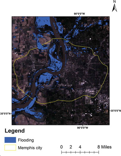
Figure 15. Spectral profile of pixels within the footprint.

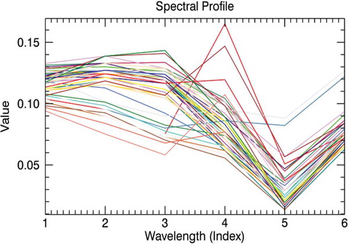
The spectral profile of a sample of pixels falling within the flood footprint (Fig. 15) shows that the footprint extracted using the present algorithm is able to identify the wet areas and sediment-laden water along with the standing flood water. The spectral profile shows the reflectance curves similar to these classes along with the water.

In the case study of the Queensland flood, thresholds of 74 and 111 were found to delineate water on pre- and post-flood event images. After comparing the images, the flood extent was delineated (Fig. 16). Using the aerial images as reference, an accuracy assessment was carried out for both the approaches. Table 4 shows the accuracy assessment results for both the techniques, i.e. using wetness transformation and thresholding of the TM4 band. The overall accuracy of the former methodology shows better performance than thresholding of TM4 imagery. The main source of inaccuracy in thresholding of the TM4 image was the error of omission (31.48%); it was observed at many places that flooded areas that could be clearly seen as flooded in aerial imagery, were missed (Fig. 17).

Table 4. Accuracy assessment results.

Parameters	Wetness transformation	TM4 thresholding
Overall accuracy (OA)	94%	88.2%
Error of omission (EO)	12.34%	31.48%
Error of commission (EC)	4.05%	6.72%

Figure 16. Queensland flood extents delineated using thresholding of the TM4 image (left), and using the wetness transformation approach (right).

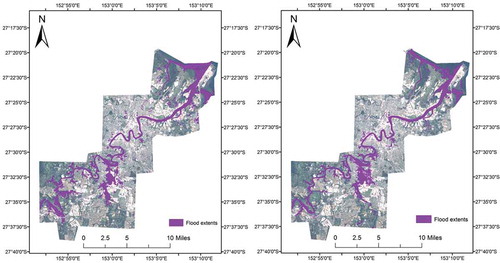
Figure 17. Flooded areas missed by thresholding of the TM4 image, Queensland.

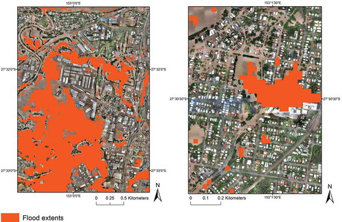
There could be two reasons for this. First, the satellite image was acquired after 4 days of the flood event and at many locations the flood water had receded and thus no water could be identified by thresholding of the TM4 image. Secondly, TM is a medium resolution sensor and in urban flooding there can be mixed pixel effects due to the presence of water, structures and other classes. In this situation, the reflectance value in the TM4 image does not represent water only. The sources of errors were found to be minimized by using the wetness transformation approach. Since the approach works on the wetness of the area, most of the errors due to the mixed pixel effect and absence of standing flood water were minimized. It can be seen that using wetness transformation, the error of omission was reduced by 19.14%.

Conclusions and future scope

In flooded urban regions where misclassification due to scattering at lower wavelengths, confusion due to presence of asphalt and sediment-laden water, as well as the receding of flood water, cause considerable challenges to accurately identifying the flood hazard footprint, the present methodology proved to be effective in minimizing most of the associated errors. Wetness transformed images have shown potential for delineating sediment-laden water and wet areas, thus providing a comprehensive flood hazard footprint. The present technique is not based on identifying water and non-water pixels; it utilizes the concept of wetness in the study area. Thus this technique can be useful even if the satellite image is acquired after 3–4 days of the flood event when the standing water has receded to a certain extent.

Another important aspect of using wetness transformed images is that it utilizes six bands of the TM imagery and consequently it reduces the error induced by the presence of asphalt when thresholding is used on near infrared bands for delineating the flood map. The present approach involves less manual effort compared to the earlier approaches. Thresholding is the only manual work carried out during the process, which makes it fast and easy to implement.

As part of future work, the wetness transformation coefficients for other sensors need to be established so that the present approach becomes sensor independent. Moreover, there are certain kernel-based automated approaches available for thresholding in the literature which may be used with the present approach. The inclusion of such kernel-based algorithms has the potential to make this process of urban flood mapping completely automated.

Disclosure statement

No potential conflict of interest was reported by the authors.

References

- Chavez, P.S., 1988. An improved dark-object subtraction technique for atmospheric scattering correction of multispectral data. Remote Sensing of Environment, 24, 459–479. doi:10.1016/0034-4257(88)90019-3
- Congalton, R.G., 1991. A review of assessing the accuracy of classifications of remotely sensed data. Remote Sensing of Environment, 37, 35–46. doi:10.1016/0034-4257(91)90048-B
- Crippen, R.E., 1988. The dangers of underestimating the importance of data adjustments in band ratioing. International Journal of Remote Sensing, 9 (4), 767–776. doi:10.1080/01431168808954891
- Crist, E.P., 1985. A TM Tasseled Cap equivalent transformation for reflectance factor data. Remote Sensing of Environment, 17, 301–306. doi:10.1016/0034-4257(85)90102-6
- Frazier, P.S. and Page, K.J., 2000. Water body detection and delineation with Landsat TM data. Photogrammetric Engineering and Remote Sensing, 66 (12), 1461–1467.
- Frey, H., et al., 2010. Automated detection of glacier lakes based on remote sensing in view of assessing associated hazard potentials. Grazer Schriften der Geographie und Raumforschung, 45, 261–272.
- Imhoff, M.L., et al., 1987. Monsoon flood boundary delineation and damage assessment using space borne imaging radar and Landsat data. Photogrammetric Engineering and Remote Sensing, 53, 405–413.
- Islam, M.M. and Sado, K., 2002. Development priority map for flood countermeasures by remote sensing data with geographic information system. Journal of Hydrologic Engineering, 7 (5), 346–355. doi:10.1061/(ASCE)1084-0699(2002)7:5(346)
- Jain, S.K., et al., 2006. Flood inundation mapping using NOAA AVHRR data. Water Resources Management, 20 (6), 949–959. doi:10.1007/s11269-006-9016-4
- Kauth, R.J., et al., 1979. Feature extraction applied to agricultural crops as seen by Landsat. In: Proceedings of LACIE symposium. Houston, TX: NASA, 705–721.
- Kauth, R.J. and Thomas, G.S., 1976. The tasselled cap—a graphic description of the spectral–temporal development of agricultural crops as seen by LANDSAT. In: Proceedings of the symposium on machine processing of remotely Sensed data. West Lafayette, IN: Purdue University, 41–51.
- QI, S., et al., 2009. Inundation extent and flood requency mapping Using LANDSAT Imagery and Digital Elevation Models. GIScience & Remote Sensing, 46 (1), 101–127. doi:10.2747/1548-1603.46.1.101
- Ridler, T.W. and Calvard, S., 1978. Picture thresholding using an interactive selection method. In: IEEE Transactions on Systems, Man, and Cybernetics.
- Singh, A., 1989. Review article digital change detection techniques using remotely-sensed data. International Journal of Remote Sensing, 10, 989–1003. doi:10.1080/01431168908903939
- Song, C., et al., 2001. Classification and change detection using Landsat TM data: when and how to correct atmospheric effects? Remote Sensing of Environment, 75 (2), 230–244. doi:10.1016/S0034-4257(00)00169-3
- Wang, Y., 2004. Using Landsat 7 TM data acquired days after a flood event to delineate the maximum flood extent on a coastal floodplain. International Journal of Remote Sensing, 25 (5), 959–974. doi:10.1080/0143116031000150022
- Wang, Y., Colby, J.D., and Mulcahy, K.A., 2002. An efficient method for mapping flood extent in a coastal floodplain using Landsat TM and DEM data. International Journal of Remote Sensing, 23 (18), 3681–3696. doi:10.1080/01431160110114484