Assessing the major drivers of water-level declines: new insights into the future of heavily stressed aquifers

ABSTRACT

The major driver of water-level changes in many heavily stressed aquifers is irrigation pumping, which is primarily a function of meteorological conditions (precipitation and potential evapotranspiration). Correlations among climatic indices, water-level changes, and pumping can thus often be used to assess the impact of climatic and anthropogenic stresses. The power of this simple, first-order approach, which captures the primary excitation–response relationships driving aquifer behavior, is demonstrated for the High Plains aquifer in the central United States (Kansas). Regional correlations between water-level changes and climatic indices indicate that a repeat of the most severe drought on record would more than double water-level decline rates. More importantly, correlations between water-level changes and reported pumping reveal that practically feasible pumping reductions should stabilize water levels, at least temporarily, over much of the aquifer in Kansas. This example illustrates that when uncertainty obscures process-based modeling projections, simple approaches such as described here can often provide insights of great practical value.

Editor D. Koutsoyiannis; Associate editor A. Fiori

KEYWORDS:

• Groundwater levels
• climatic index
• groundwater pumping
• High Plains aquifer

Introduction

The question of what the future holds for heavily stressed aquifers is of great societal interest. This is particularly true in areas that are prone to or have recently experienced severe droughts, such as the Great Plains region of the United States (US). Changes in water levels have long served as a measure of an aquifer’s response to anthropogenic and climatic stresses. Records of past changes, however, just tell us where we have been; the more critical issue is where we are going.

Approaches for forecasting water-level changes have ranged from extrapolation of past trends (e.g., Fig. 7 in Buchanan et al. 2015) to process-based modeling (e.g., Anderson and Woessner 1991). Intermediate between these two end members are data-based methods of varying degrees of complexity that are focused on exploiting relationships between water-level changes and potential drivers of those changes (e.g., Chen et al. 2002, Gurdak et al. 2007, Adamowski and Chan 2011, Sahoo and Jha 2013). A subset of these intermediate methods is based on correlations between water-level changes and possible causative factors (e.g., Chen et al. 2004). If these relatively simple correlation-based approaches can explain most of the observed changes, they can serve as valuable tools for rapid, first-order assessment of an aquifer’s response to various pumping and climatic scenarios. One such approach is discussed here and applied to a portion of one of the world’s largest aquifer systems, the High Plains aquifer (HPA) of the central US.

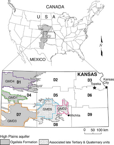
The HPA extends over portions of eight states in the Great Plains region of the US (Fig. 1) and provides irrigation and, to a much lesser extent, drinking, stock, and industrial water supplies that account for nearly one-quarter of the nation’s annual groundwater use (Maupin and Barber 2005). Much of the aquifer system, however, appears to be on a fundamentally unsustainable path. Large pumping-induced declines (Stanton et al. 2011), which have been the focus of recent articles in the popular media (e.g., Wines 2013), indicate that current rates of withdrawals cannot be sustained; the projected trajectory of climate change further exacerbates the situation (e.g., Rosenberg et al. 1999, 2003, Brunsell et al. 2010, Logan et al. 2010).

Figure 1. Map of the High Plains aquifer in the US and Kansas (inset). Kansas inset also shows groundwater management district (GMD – colored lines) and climatic division (dashed) boundaries (modified from Butler et al. 2013).

The main driver of water-level changes in the HPA is the amount of water pumped for irrigation (making up approximately 95% of total pumped in 2005 [Kenny et al. 2009]). Irrigation is primarily needed to supplement precipitation for fall-harvested row crops, so pumpage is concentrated in the summer growing season. The volume of irrigation pumpage is determined by the number of wells and the amount pumped per well. For a given hydrostratigraphic configuration, the primary controls on the per-well amount include the area irrigated, meteorological conditions (i.e. precipitation and potential evapotranspiration), crop type, and regulatory (water-right) allocation. If the number of wells, irrigated area, crop mix, and water-right allocation remain relatively constant, then the main factor controlling pumping is the meteorological conditions for a given year.

Climatic indices provide a good measure of meteorological conditions, especially how precipitation deviates from historic norms. Commonly used indices include the Palmer Drought Severity Index (PDSI), the Palmer Z Index, and the Standardized Precipitation Index (SPI). The PDSI is a monthly index calculated using precipitation, soil moisture, potential evapotranspiration, and other factors important to plant growth (Palmer 1965). The Palmer Z Index is a similar monthly index developed to evaluate short-term moisture conditions in crop-producing areas; the PDSI, in comparison, was developed to monitor longer-term wet and dry spells (Heim 2002). The SPI was created to quantify precipitation deficits and surpluses (normalized by long-term records) over time intervals of practical relevance for water resources (McKee et al. 1993). Although there are a number of other climatic indices, such as the recently proposed Standardized Precipitation Evapotranspiration Index (Vicente-Serrano et al. 2010), these have not been as widely used as the Palmer indices and SPI. Monthly values of PDSI, Palmer Z Index, and SPI (for various intervals) are available online for climatic divisions of US states (National Climatic Data Center 2014).

The major objective of this paper is to demonstrate how relationships among climatic indices, water-level changes, and reported water use can be simply and quickly exploited to develop new insights into the future of heavily stressed aquifers. The focus is on the relatively data-rich portion of the HPA in the state of Kansas, but the general procedure should be widely applicable. This approach is not envisioned as a replacement for process-based modeling. However, in cases where uncertainty produced by limited data and incomplete mechanistic descriptions may obscure process-based modeling projections, simple approaches such as that described here, which capture the primary excitation–response relationships driving large-scale system behavior, can be of great practical value.

The High Plains aquifer in Kansas

The HPA extends over the western third and the south-central parts of the state of Kansas (Fig. 1) and is overlain by five groundwater management districts (GMDs). The areas of the three western districts (from north to south, GMDs 4, 1, and 3) coincide well with the western three (1, 4, and 7, respectively) of the state’s nine climatic divisions; the areas of GMDs 2 and 5 (henceforth, GMDs 2&5) in south-central Kansas are predominately located within climatic division 8 and will be considered together for the purposes of this work (Fig. 1). A climatic division is an area of relatively uniform climatic characteristics for which climatic data are reported monthly by the National Climatic Data Center (NCDC 2014); the divisions were created in 1950 and correspond to the Crop Reporting Districts of the United States Department of Agriculture. The three western Kansas climatic divisions are characterized by semi-arid conditions, while the south-central Kansas climatic division is characterized by a more sub-humid climate.

Groundwater levels in the Kansas HPA have been measured annually in an extensive well network for several decades. The network currently consists of about 1400 wells distributed approximately evenly over the aquifer (Miller et al. 1999, Bohling and Wilson 2012). The measurements are made during the winter when irrigation wells are typically not operating. In the mid-1990s, the Kansas Geological Survey took over primary responsibility for managing the measurement program; the data collected since that time (1996) are utilized here.

Data from the Kansas well network can be used to calculate spatial averages of the annual changes in water level for each of the GMD regions for 1996–2012 (where the value for a particular year represents the average difference between the winter water-level measurements in that year and the following year). The patterns of the annual changes for the western three GMDs are relatively similar, showing declines in most years (Fig. 2(a)). The infrequent small annual rises primarily represent greater aquifer recovery at the time of the winter water-level measurement (result of less water use and/or earlier cessation of pumping in the previous irrigation season) rather than recharge of same-year precipitation (depth to the water table in these areas is substantial and the estimated mean annual recharge is small, <1–2 cm under natural [non-irrigated] conditions, due to relatively low mean annual precipitation [40–58 cm] and high evapotranspiration [Fross et al. 2012]). The much more frequent and substantial annual rises in water levels in south-central Kansas (GMDs 2&5) do mainly reflect recharge of same-year precipitation because the mean annual precipitation is greater (58–84 cm) and the average depth to water is much less. The patterns of annual changes observed in the 1996–2012 data are also observed in long-term hydrographs from wells in the GMDs. The HPA in the three western GMDs has been so heavily stressed by pumping since the 1950s that the vast majority of hydrographs show substantial declines over the last half century, indicating that the aquifer is being mined. Declines are appreciably less in GMDs 2&5; the hydrographs fluctuate substantially from year to year but with a much smaller long-term trend than farther west, reflecting pumping activity as well as aquifer recharge and stream–aquifer interactions.

Figure 2. (a) Mean annual water-level changes (solid lines) in the HPA in the GMD areas and SPI 9-month October (GMDs 4, 1, and 3) and 12-month December (GMDs 2&5) values (dashed lines) during 1996–2012. See Fig. 1 for the locations of the climatic divisions and GMDs. The y-axis ranges vary among plots to accentuate the relationship between fluctuations in water-level change (left y-axis) and those in the SPI (right y-axis). Water-level data are from wells for which measurements are available throughout 1996–2013 (188, 60, 222, and 233 wells for GMDs 4, 1, 3, and 2&5, respectively). A value for a particular year represents the water-level difference between that year and the following year for a given well; the mean annual change is an unweighted arithmetic average of the values for all the wells. A SPI value of zero indicates average (historic norm) conditions, values <0 and >0 indicate dry and wet conditions, respectively. (b) Correlation plots for data displayed in (a). See Table 1 for coefficients of determination and regression equations. The point within the circle in (b) is the outlier referred to in the text.

Development of the Kansas HPA and expansion of irrigated cropland was substantial during the middle part of the 20th century. However, since the mid-1990s, the irrigated area and crop types in Kansas have not changed appreciably (Rogers and Lamm 2012) and the number of water-right permitted irrigation wells has increased only slightly (~6%). In addition, Hendricks and Peterson (2012) found that irrigation pumping in Kansas for 1992–2007 varied little in response to fluctuations in energy prices. Thus, the main driver for water-level changes in the Kansas HPA during this period was the pumping induced by meteorological conditions.

Correlation of water-level change with climatic indices and water use

Climatic indices

Temporal variations in mean annual water-level changes parallel the temporal variations in climatic indices for the GMD areas (e.g., Fig. 2(a)). This implies a high degree of correlation between the water-level changes and the climatic indices, which is confirmed by linear-regression analyses (Fig. 2(b), Table 1). Although irrigation pumping is expected to be tied most closely to conditions during the growing season (typically May through early September), some of the best correlations were obtained for a range of months exceeding the growing season for the PDSI and Palmer Z Index, and for 9-month and 12-month SPI values (Table 1). This is thought to be partly related to pre-planting irrigation to increase soil moisture and, where the water table is shallow, recharge of same-year precipitation and stream–aquifer interactions. Although the Palmer indices, which incorporate precipitation and temperature, and involve calculations of evapotranspiration (ET) and soil moisture, give high correlations with water-level changes, the SPI gives correlations nearly as high as or higher than those for the Palmer indices (Table 1). This indicates that precipitation variations are the main climatic driver of water-level change across the Kansas HPA. However, the mechanisms that produce the high correlation with precipitation vary across the Kansas HPA. In the western Kansas GMDs, except for during and shortly after a precipitation event, pumping of groundwater is essentially continuous throughout the irrigation season (e.g., Figs 2 and 3 of Butler et al. 2013). Thus, precipitation controls when the pumps are operating, and therefore is an indirect control on water levels. In the south-central Kansas GMDs, this mechanism is supplemented by recharge of recent precipitation; in those areas, precipitation has both a direct and indirect control on water levels. More efficient use of water (irrigation done only during critical periods of high ET demand) would likely improve the correlations involving the Palmer indices in all the GMDs.

Figure 3. (a) Mean annual water-level changes (solid lines) and reported water use (dashed lines) for the HPA in the GMD areas during 1996–2012. See Fig. 1 for the locations of the climatic divisions and GMDs; the y-axis ranges vary among plots to accentuate the relationship between fluctuations in water-level change (left y-axis) and those in water use (right y-axis). The water-level data are the same as shown in Fig. 2(a). (b) Correlation plots for data displayed in (a). See Table 2 for coefficients of determination and regression equations. The point within the circle in (b) is the outlier referred to in the text.

Table 1. Optimum^a and utilized^b (bolded) correlations of mean annual water-level changes for GMDs with climatic indices for coinciding climatic divisions during 1996–2012.

Climatic index	GMD and Climatic Division	R^2
PDSI, August	GMD4–Div. 1	0.739
Palmer Z, mean Jun.–Sep.	GMD4–Div. 1	0.822
SPI, 9-month, December	GMD4–Div. 1	0.831
SPI, 9-month, October^c	GMD4–Div. 1	0.781
Water-level change (m) = 0.1409  × SPI – 0.182
PDSI, mean Aug.–Nov.	GMD1–Div. 4	0.463
Palmer Z, mean Jun.–Nov.	GMD1–Div. 4	0.656
SPI, 9-month, October^c	GMD1–Div. 4	0.709
Water-level change (m) = 0.1524  × SPI – 0.171
PDSI, mean Jun.–Dec.	GMD3–Div. 7	0.833
Palmer Z, mean Apr.–Nov.	GMD3–Div. 7	0.830
SPI, 9-month, November	GMD3–Div. 7	0.800
SPI, 9-month, October^c	GMD3–Div. 7	0.776
Water-level change (m) = 0.3166  × SPI – 0.584
PDSI, mean Jul.–Oct.	GMD 2&5–Div. 8	0.744
Palmer Z, mean Jan.–Dec.	GMD 2&5–Div. 8	0.794
SPI, 12-month, December^d	GMD 2&5–Div. 8	0.782
Water-level change (m) = 0.4528  × SPI – 0.283

^aOptimum correlation determined for each of the climatic indices (PDSI, Palmer Z, and SPI).

^bLinear regression equations are listed for the utilized correlations. All R² (coefficient of determination) values are significant at P = 0.001 except that for GMD1 water-level change vs PDSI division 4, which is significant at P = 0.01.

^cIndex based on 9-month period ending with October.

^dIndex based on 12-month period ending with December.

The focus of this paper is on the correlation with the SPI, not just because it is the simplest of the common climatic indices, but it is also the only climatic index that gives coefficient of determination (R²) values greater than 0.7 for all of the GMD areas of the Kansas HPA. The period of the SPI index that produces the optimum correlation with annual water-level changes differs slightly among the three western GMDs. In order to facilitate comparisons, the SPI, 9-month, October index is used here for the three western GMDs. The slight decreases in the correlations for GMDs 4 and 3 (Table 1) resulting from use of this form of the SPI are not of practical importance. A different index (SPI, 12-month, December) is used for the GMDs 2&5 area, which is characterized by greater precipitation and recharge of same-year precipitation.

The correlations between the SPI and the annual water-level changes are high for all of the GMD areas, but the correlation is somewhat weaker for GMD1 (Table 1). The likely explanation for this lower correlation, which undoubtedly explains a considerable portion of the spread observed in all the correlation plots (Fig. 2(b)), is the distribution of rainfall within the period covered by the SPI. For example, if the circled outlier point in Fig. 2(b) (water-level change of +0.19 m and an SPI of 0.86) is removed from the GMD1 data, the R² for the correlation increases from 0.71 to 0.80. Precipitation in GMD1 for that year (1997) was higher than the 1996–2012 average for the three months when irrigation water demand by crops is generally the highest (June–August). Thus, pumping was likely considerably less than expected for the typical irrigation season and concentrated much earlier in the season, leading to a year-on-year increase in winter water levels. Also, the distribution of the rainfall was such that the SPI value was not as high as it would have been if the precipitation had been more evenly distributed throughout the 9-month period.

Water use

Since 1978, Kansas has required non-domestic water users to obtain a water right. Starting in the early 1980s, water-right holders were required to submit annual water-use reports; quality control of the reported data began in 1990. Variations in annual water-level change are generally of opposite sign to those of water use during 1996–2012 (Fig. 3(a)), as would be expected. Correlations of annual water-level changes with reported water use during 1996–2012 for GMDs 4 and 2&5 are high, although not quite as high as with the SPI; the correlation for GMD3 is statistically significant but substantially lower than that with the SPI, whereas that for GMD1 is not statistically significant (Fig. 3(b), Table 2). If the circled outlier value (2007 – water-level change of +0.86 m and water use of 0.72 × 10⁹ m³) is removed from the data for GMDs 2&5, the R² improves to 0.88, a remarkably high correlation; that outlier is again a result of the distribution of precipitation during the growing season. The most likely explanation for the weaker correlations between water-level changes and water use for GMDs 1 and 3 is the greater use of less-accurate meters (e.g., duration-of-pumping vs flow-rate meters) in those districts. A second explanation is downward trends in the annual water-level change data that are not consistent with the water-use data. GMD3 has a downward trend in the annual water-level change data but no trend in water-use data. If a linear trend is removed from the water-level change data, the correlation increases from 0.32 to 0.56 (statistically significant at the P = 0.01 level). An explanation for the downward trend is that it is a product of changes in hydrostratigraphic conditions, specifically decreasing specific yield and/or increasing aquifer compartmentalization, as has been reported elsewhere for the western Kansas HPA (Butler et al. 2013). Such hydrostratigraphic changes with depth are not unexpected in this portion of the HPA as the sedimentary sequence transitions from one dominated by sands and gravels (channel deposits) to one dominated by clays and silts (inter-channel deposits) as discussed by Butler et al. (2013). An additional possibility for the weaker correlation in GMD3 is that the Arkansas River valley and surface irrigation districts fed by the river provide supplemental irrigation water that is not available in the other districts. GMD1 has downward trends in both water-level change and water-use data. If linear trends are removed from both data sets, the correlation increases from an R² of 0.07 to 0.47 (statistically significant at the P = 0.01 level). The downward trend in the water-level change data could be a product of changing hydrostratigraphic conditions, while the downward trend in the annual pumping could be due to diminishing transmissivity with decreasing saturated thickness (i.e., the drawdown produced by the lower transmissivity limits pumping at individual wells). Neither GMD4 nor GMDS 2&5 have trends in water-level change that are inconsistent with the water-use data.

Table 2. Coefficients of determination (R²) and linear regression equations for correlation of mean annual water-level changes with reported water use during 1996–2012 for the GMD areas^a.

GMD	R^2	Equation
GMD4	0.732	Water-level change (m) = −1.60 × 10^-9 × water use (m^3) + 0.664
GMD1	0.068	Water-level change (m) = −1.01 × 10^-9 × water use (m^3) + 0.131
GMD3	0.318	Water-level change (m) = −0.706 × 10^-9 × water use (m^3) + 1.17
GMDs 2&5	0.765	Water-level change (m) = −2.44 × 10^-9 × water use (m^3) + 2.02

^aCorrelations for GMD4 and GMDs 2&5 are statistically significant at P = 0.001 and for GMD3 at P = 0.02; the correlation is not statistically significant for GMD1.

Variations in SPI are generally of opposite sign of those of water use during 1996–2012 (Fig. 4(a)), as would also be expected. Correlations of SPI with reported water use for GMDs 4 and 2&5 are high, although not as high as with annual water-level change; the correlation for GMD3 is statistically significant but substantially lower than that with water-level change, whereas that for GMD1 is not statistically significant (Fig. 4(b)). As for the relationship between water-level change and water use described above, if the water-level change data are detrended, the R² values for GMDs 1 and 3 increase.

Figure 4. (a) SPI 9-month October (GMDs 4, 1, and 3) and 12-month December (GMDs 2&5) values (solid lines) and reported water use (dashed lines) for the HPA in the GMD areas during 1996–2012. See Fig. 1 for the locations of the climatic divisions and GMDs; the y-axis ranges vary among plots to accentuate the relationship between fluctuations in SPI (left y-axis) and those in water use (right y-axis). The SPI data are the same as shown in Fig. 2(a) and the water use data the same as in Fig 3(a). (b) Correlation plots and R² values for data displayed in (a).

In general, the water-level data set has the least uncertainty of the three data types considered here because the data set is based on annual measurements taken at the same time of the year at the same location in a regular network across the HPA. The climatic data set is expected to have greater uncertainties because measurement locations are fewer in number and less regularly distributed than the water-level data, and different temporal patterns in precipitation can give similar climatic index values for a particular period. Given the time frame of this assessment, changes in measurement methods for climatic data and in the duration and intensity of rainfall events are not expected to introduce significant uncertainty relative to that produced by the number and distribution of measurement locations and the distribution of precipitation during the period characterized by SPI values. The data set with the greatest uncertainty is reported water use. The relative uncertainties in the three data sets are reflected in the general relative order of correlation strength among the data sets: highest for SPI vs water-level change, followed by water use vs water-level change, and lowest for water use vs SPI.

Prediction of future water-level changes

The strength of the correlations discussed in the previous section indicates that these relationships can be exploited to develop insights into the HPA response to various future scenarios. We demonstrate the value of this approach through an assessment of the predicted response to the cases of extended drought, continuation of average climatic conditions, and reductions in pumping. Given the illustrative nature of this paper, the predicted responses are presented without confidence intervals, i.e. response should be considered the mean response for the defined conditions.

Extended drought

The 1930s and 1950s had the longest and most severe years of recorded drought in Kansas (Paulson et al. 1991). Although the 1930s drought extended for a longer period than that for the 1950s, the 1950s drought included years (particularly 1956) with the most severe drought conditions since record keeping began in 1895. The SPI values for past drought periods can be used in the regression equations of Table 1 to predict annual water-level declines for each of the GMD areas. Applying this procedure to a drought of the same length (5 years) and intensity of the 1950s drought, which occurred prior to widespread irrigation pumping in the Kansas HPA, yields total water-level declines of 2.01, 2.05, 5.06, and 5.07 m for GMDs 4, 1, 3, and 2&5, respectively (Table 3). The mean annual declines predicted for a repeat of the 1950s drought range from 1.8 to 2.6 times those observed during 1996–2012 for the three western GMDs, and even greater for GMDs 2&5. A repeat of this extended drought would clearly have an extremely deleterious impact on conditions in the Kansas HPA.

Table 3. SPI values for given year and predicted water-level declines calculated using the regression equations in Table 1 for a drought of the same length and intensity of that of the 1950s.

Year	GMD4		GMD1		GMD3		GMDs 2&5
	SPI 9-month October	Predicted decline (m)	SPI 9-month October	Predicted decline (m)	SPI 9-month October	Predicted decline (m)	SPI 12-month December	Predicted decline (m)
1952	−1.62	−0.41	−1.70	−0.43	−1.92	−1.19	−1.46	−0.94
1953	−0.53	−0.26	−1.02	−0.33	−1.14	−0.94	−1.36	−0.90
1954	−1.47	−0.39	−1.46	−0.39	−1.26	−0.98	−2.16	−1.26
1955	−1.66	−0.42	−0.78	−0.29	−0.01	−0.59	−0.62	−0.56
1956	−2.49	−0.53	−2.87	−0.61	−2.44	−1.36	−2.47	−1.40
Total		−2.01		−2.05		−5.06		−5.07

Global climate models project that winter precipitation will increase slightly in western Kansas but spring precipitation will decrease and summer precipitation will decrease even more (Brunsell et al. 2010). These projections indicate that lower SPI values will be more common in the coming decades and that the frequency of droughts similar to that of the 1950s may increase. The above assessment indicates that such conditions will likely lead to an acceleration of water-level declines across all portions of the HPA in Kansas.

Average climate

The zero value for a climatic index indicates average (historic—since 1895 for Kansas—norm) conditions. The water-level change at the zero value thus provides insight into how pumping is affecting water levels under conditions that would be considered neither wet nor dry for a particular area. The annual water-level changes at the zero SPI value are negative (water-level declines) for all GMDs during 1996–2012: −0.18 m for GMD4, −0.17 m for GMD1, −0.58 m for GMD3, and −0.28 m for GMDs 2&5 (intercept values in regression equations in Table 1). The declines for the three western GMDs are not unexpected because the natural recharge to the HPA in these areas is very small relative to the amount of pumping (Fross et al. 2012), i.e. the aquifer is being mined under average climatic conditions.

GMDs 2&5 are attempting to manage their areas on a long-term sustainable basis, so the 0.28 m/year decline is surprising. However, the actual decline rate over 1996–2012 was much less (0.07 m/year) because the climatic conditions for this period were slightly wetter than average (historic norm). The 1996–2012 mean of the SPI index for GMDs 2&5 is 0.47, which is on the wet side of normal. In contrast, the SPI means for climatic divisions 1, 4, and 7 are very close to zero (−0.01, 0.11, and 0.08, respectively) for this same period. This implies that, should the mean of future climatic conditions be closer to an SPI of zero for GMDs 2&5, unexpected water-level declines could occur even during normal meteorological conditions. The annual water-level data (Fig. 2(a)) and hydrographs from continuously monitored wells (e.g., Fig. 3 in Butler et al. 2011) are consistent with this projection, as both indicate that GMDs 2&5 are dependent on substantial but infrequent recharge events to sustain water levels. A decrease in the frequency of such events would lead to further declines even without the onset of drought conditions.

Reductions in pumping

Given that water-level declines are expected to continue across the Kansas HPA under average climatic conditions, there is growing interest in reducing pumping to extend the “usable lifetime” of the aquifer. The key question is how much reduction is needed to significantly moderate the declines. A new management framework, the Local Enhanced Management Area (LEMA), was established by the Kansas Legislature in 2012 to allow the adoption of locally generated management plans that are supported by regulatory oversight (Kansas Department of Agriculture 2013). In January 2013, the first LEMA was established in a 256-km² area within GMD4; the management plan calls for a reduction in average annual pumping of about 20% over a period of 5 years in the hope that that would produce a significant reduction in the rate of water-level decline.

An obvious question is what percentage reduction would produce a stabilization of water levels across the entire GMD4 area. If, as in GMD4, reliable water-use (groundwater pumping) data are available, then the water use vs annual water-level change relationship (Table 2) can be utilized to assess this issue. The approach (Table 4) yields a pumping reduction of 22%, which is quite close to the target reduction for the first LEMA in Kansas. Thus, it appears that a practically feasible reduction in annual pumping would have kept water levels (in terms of the regional average) at approximately the same level from 1996 to 2012. However, the reduction is much smaller than expected for long-term sustainability. This finding suggests that there is a previously unrecognized inflow to the HPA within GMD4 and is consistent with the recent interpretation of hydrographs from some continuously monitored wells in that area (e.g., Butler et al. 2013). The source of the inflow and its expected duration are the focus of ongoing investigations; it likely is a short-term phenomenon related to irrigation return flow and delayed drainage from the unsaturated zone created by water-level declines.

Table 4. Steps for calculating pumping reduction to obtain stable water levels (water-level change of zero) for GMD4 and GMDs 2&5 during 1996–2012 using water-level and water-use regression equations in Table 2.

Percentage reduction in water use required for stable water levels under observed climatic conditions

GMD4: Water-level change (m) = 0 = −1.60 × 10^-9 × water use (m^3) + 0.664

Water use = −0.664/(−1.60 × 10^-9) = 4.14 × 10^8 m^3

Average annual reported water use for 1996–2012 = 5.28 × 10^8 m^3

Percentage reduction in water use = ((5.28 − 4.14)/5.28) × 100 = 21.7%

GMDs 2&5: Water-level change (m) = 0 = −2.44 × 10^-9 × water use (m^3) + 2.02

Water use = −2.02/(−2.44 × 10^-9) = 8.27 × 10^8 m^3

Average annual reported water use for 1996–2012 = 8.57 × 10^8 m^3

Percentage reduction in water use = ((8.57 − 8.27)/8.57) × 100 = 3.4%

The pumping reduction required to stabilize water levels for GMDs 2&5 can be calculated in a similar manner. Given that climatic conditions have been slightly wetter than the historic norm in this area for 1996–2012, a pumping reduction of approximately 3% from the average for that period would produce near-stable water levels (Table 4). However, if climatic conditions had been the historic average for this period, a larger pumping reduction (17%) would be required for stabilization (calculation based on a water-level change of +0.28 m to achieve stable water levels at an SPI value of zero using the approach of Table 4).

The poor correlations between water use and annual water-level change preclude the direct application of the regression for assessing reduction impacts for GMDs 1 and 3. However, an approximate approach can be applied to GMD1 by recognizing that a reduction in water use is equivalent (in terms of its impact on water-level changes) to the occurrence of a wetter period (i.e. greater SPI value) and then determining that equivalence using data from GMD4. This approach can be justified by the high degree of similarity between the linear regressions for water-level change vs SPI for GMDs 1 and 4 (Table 1), which is undoubtedly due to the similarities in irrigated crops and irrigation practices in these two adjacent GMDs. The 22% water-use reduction in GMD4 is equivalent to a SPI change of 1.30 (−0.01 to 1.29, Table 5a). If the same relationship between percentage pumping reduction and SPI change is assumed, the strong correlation between climatic indices and annual water-level change for GMD1 can be exploited to assess the impact of a pumping reduction for GMD1. Using the same SPI change as in GMD4, an annual water-level increase of 0.04 m is obtained for GMD1 (Table 5b). Thus, a reduction in annual pumping of about 20% would have likely kept the average of water levels in GMD1 at approximately the same level for the entire period. The dissimilarity between the linear regressions for water-level change vs SPI for GMDs 3 and 4 precludes the application of this approach to GMD3.

Table 5. Steps for calculating average annual water-level decline for 21.7% reduction in pumping in GMD1 based on SPI change for this reduction in GMD4 for 1996–2012.

a. SPI change corresponding to 21.7% pumping reduction in GMD4

Insert water-level change of zero for reduced pumping into regression equation in Table 1

Water-level change (m) = 0 = 0.141 × SPI – 0.182

SPI = 0.182/0.141 = 1.29

Average SPI (9-month October) for 1996–2012 = −0.011

SPI change corresponding to pumping reduction = 1.29−(−0.011) = 1.30

b. Compute average annual water-level change for GMD1 for SPI change of 1.30

Use regression equation in Table 1 for GMD1

Water-level change (m) = 0.152 × SPI – 0.171

Average SPI (9-month, October) for climatic division 4 (GMD1) = 0.105

SPI for change of 1.303 = 0.105 + 1.303 = 1.408

Water-level change (m) = 0.152 × 1.41 − 0.171 = 0.044 m

Average annual water-level change observed for 1996–2012 = −0.155 m

Reduction in average annual water-level decline = 0.044 − (−0.155) = 0.199 m

The reductions in pumping that would stabilize groundwater levels can be used to estimate mean annual recharge rates to the HPA in GMDs 1 and 4 because groundwater discharge to streams in these areas has been insignificant over the last few decades. Dividing the volume of pumping that would stabilize groundwater levels by the GMD area gives mean recharge rates of 4.7 and 3.3 cm/year for GMDs 1 and 4, respectively, which are three to four times greater than other estimated recharge values for these GMDs (e.g., Fross et al. 2012). These rates represent the volume of pumping averaged over the entire GMD area. In actuality, the pumping volume is concentrated in those areas where the pumping occurs (and where most of the water-level measurements are made); use of the area of influence of the pumping wells in the recharge calculation would lead to a substantially larger recharge rate. A similar approach cannot be used to estimate the mean annual recharge in GMDs 2&5 because of the large amount of groundwater discharge to streams in those areas.

Conclusions

The major driver of water-level changes in many heavily stressed aquifers is the amount of water pumped for irrigation. Thus, correlations among climatic indices, changes in water levels, and reported water use can often serve as valuable tools for assessing an aquifer’s response to various climatic and development scenarios. Projections of future climatic conditions can be defined in terms of climatic indices; these indices can then be used in a linear regression (climatic index vs annual water-level change) to assess an aquifer’s likely response to those conditions. The magnitude of the intercept of the regression can shed light on aquifer sustainability at average climatic conditions under current pumping practices. If water-use (groundwater pumping) data are available for at least a portion of the area or nearby areas, pumping vs annual water-level change regressions can be used to develop difficult-to-obtain insights into the impact of pumping reductions on the rate of water-level declines. Even when pumping data are not available, some sense of the magnitude of pumping reductions required to significantly moderate declines can be obtained by recognizing that the aquifer response to a pumping reduction would be similar to the response to a wetter climatic period.

This simple approach has great potential for widespread application, especially for aquifers that have been fully developed (little change in area irrigated by groundwater). That potential is demonstrated through an application to a portion (state of Kansas) of the High Plains aquifer (HPA) in the central United States. The high correlation between average annual water-level changes and climatic indices across the HPA in Kansas during the past two decades confirms that pumping is primarily a function of the meteorological conditions (precipitation and potential evapotranspiration) for a given year. A precipitation-based climatic index can explain as much of the variation in water-level changes as more involved indices that incorporate potential evapotranspiration and soil moisture because of current pumping practices (near-continuous pumping during the irrigation season). These correlations indicate that a repeat of the most severe drought over the last century would have an extremely deleterious impact on the Kansas portion of the HPA under current pumping practices, as such a drought would more than double the mean rate of water-level decline. Given the potential for increased drought frequency in the coming decades, the prospects for sustaining the current rates of pumping in this portion of the HPA are not bright. Even under a future characterized by a continuation of average (historic norm) climatic conditions, water levels will continue to decline 0.2–0.6 m annually under current pumping practices. However, a key finding of this assessment is that practically feasible pumping reductions (~20%) would likely stabilize water levels, at least in the short term, over much of the Kansas HPA (Groundwater Management Districts 1, 2, 4, and 5). Although in western Kansas this stabilization may largely be a product of enhanced recharge produced by past inefficient irrigation practices and of delayed drainage from the unsaturated zone produced by water-level declines, and thus only of limited duration, it could help extend the usable lifetime of the resource and serve as a bridge to an economy based on a different mix of agricultural practices.

The correlations used here involve quantities averaged or summed over relatively large geographical areas. Thus, given the strength of these correlations, it is possible that similar correlations involving climatic indices and the large areal averages of water-level change determined from gravity measurements of the GRACE satellite mission (e.g., Strassberg et al. 2007, Famiglietti et al. 2011) could provide important insights for many heavily stressed regional aquifer systems.

In closing, we must emphasize that the approach outlined here is not envisioned as a replacement for process-based modeling. Rather, it should be viewed as a complementary tool for rapid, first-order assessment of an aquifer’s future in the face of continuing anthropogenic and climatic stresses. Such assessments should prove to be of considerable practical value for those responsible for the management of declining groundwater resources.

Disclosure statement

No potential conflict of interest was reported by the author(s).

Acknowledgement

Any opinions, findings, and conclusions or recommendations expressed in this material are those of the authors and do not necessarily reflect the views of the KWO or NSF. This paper greatly benefitted from the review provided by Garth van der Kamp.

Additional information

Funding

This work was supported, in part, by the Kansas Water Office (KWO) under contract 11-0128, the Kansas Water Plan under the Ogallala-High Plains Aquifer Assessment Program, and the National Science Foundation (NSF) under award 1039247.

References

- Adamowski, J. and Chan, H.F., 2011. A wavelet neural network conjunction model for groundwater level forecasting. Journal of Hydrology, 407, 28–40. doi:10.1016/j.jhydrol.2011.06.013
- Anderson, M.P. and Woessner, W.W., 1991. Applied groundwater modeling: Simulation of flow and advective transport. San Diego, CA: Academic Press, 381 pp.
- Bohling, G.C. and Wilson, B.B., 2012. Statistical and geostatistical analysis of the Kansas High Plains water-table elevations, 2012 measurement campaign. Lawrence: Kansas Geological Survey, Open-File Report 2012–16.
- Brunsell, N.A., et al., 2010. Seasonal trends in air temperature and precipitation in IPCC AR4 GCM output for Kansas, USA: evaluation and implications. International Journal of Climatology, 30, 1178–1193.
- Buchanan, R.C., Wilson, B.B., Buddemeier, R.R., and Butler, Jr., J.J., 2015. The High Plains aquifer. Lawrence: Kansas Geological Survey, Public Information Circular 18. Available from: www.kgs.ku.edu/Publications/pic18/index.html [Accessed 22 August 2015].
- Butler, J.J., Jr., et al., 2011. New insights from well responses to fluctuations in barometric pressure. Ground Water, 49 (4), 525–533. doi:10.1111/j.1745-6584.2010.00768.x
- Butler, J.J., Jr., et al., 2013. Interpretation of water-level changes in the High Plains aquifer in western Kansas. Groundwater, 51 (2), 180–190. doi:10.1111/j.1745-6584.2012.00988.x
- Chen, Z., Grasby, S.E., and Osadetz, K.G., 2002. Predicting average annual groundwater levels from climatic variables: an empirical model. Journal of Hydrology, 260, 102–117. doi:10.1016/S0022-1694(01)00606-0
- Chen, Z., Grasby, S.E., and Osadetz, K.G., 2004. Relation between climate variability and groundwater levels in the upper carbonate aquifer, southern Manitoba, Canada. Journal of Hydrology, 290, 43–62. doi:10.1016/j.jhydrol.2003.11.029
- Famiglietti, J.S., et al., 2011. Satellites measure recent rates of groundwater depletion in California’s Central Valley. Geophysical Research Letters, 38, L03403. doi:10.1029/2010GL046442
- Fross, D., et al., 2012. Kansas High Plains Aquifer Atlas [online]. Lawrence, KS, Kansas Geological Survey. Available from: www.kgs.ku.edu/HighPlains/HPA_Atlas/index.html [Accessed 22 August 2015].
- Gurdak, J.J., et al., 2007. Climate variability controls on unsaturated water and chemical movement, High Plains aquifer, USA. Vadose Zone Journal, 6 (3), 533–547. doi:10.2136/vzj2006.0087
- Heim, R.R., Jr., 2002. A review of twentieth-century drought indices used in the United States. Bulletin of the American Meteorological Society, 83, 1149–1165.
- Hendricks, N.P. and Peterson, J.M., 2012. Fixed effects estimation of the intensive and extensive margins of irrigation water demand. Journal of Agricultural and Resource Economics, 37 (1), 1–19.
- Kansas Department of Agriculture, 2013. Local Enhanced Management Areas (LEMA) [online]. Topeka, KS. Available from: http://agriculture.ks.gov/divisions-programs/dwr/managing-kansas-water-resources/local-enhanced-management-areas/lists/lemas/sheridan-county-6-lema [Accessed 22 August 2015].
- Kenny, J.F., et al., 2009. Estimated use of water in the United States in 2005. Washington, DC: U.S. Geological Survey Circular 1344, 60 p.
- Logan, K.E., et al., 2010. Assessing spatiotemporal variability of drought in the U.S. central plains. Journal of Arid Environments, 74, 247–255. doi:10.1016/j.jaridenv.2009.08.008
- Maupin, M.A.and Barber, N.L., 2005. Estimated withdrawals from principal aquifers in the United States, 2000. Washington, DC: U.S. Geological Survey, Circular 1279, 46 p.
- McKee, T.B., Doesken, N.J., and Kleist, J., 1993. The relationship of drought frequency and duration to time scales. In: Preprints, 8th Conference on Applied Climatology, 17–22 January 1993, Anaheim, CA, 179–184. Boston, MA: American Meteorological Society.
- Miller, R.D., Buchanan, R.C., and Brosius, L., 1999. Measuring water levels in Kansas [online]. Lawrence: Kansas Geological Survey, Public Information Circular 12. Available from: http://www.kgs.ku.edu/Publications/pic12/pic12_1.htm [Accessed 22 August 2015].
- National Climatic Data Center, 2014. Available from: www7.ncdc.noaa.gov/CDO/CDODivisionalSelect.jsp [Accessed 22 August 2015].
- Palmer, W.C., 1965. Meteorological drought. Washington, DC: U.S. Weather Bureau, NOAA Library and Information Services Division, Research Paper No. 45.
- Paulson, R.W., et al., 1991. National water summary 1988-89: hydrologic events and floods and droughts. Washington, DC: U.S. Geological Survey, Water-supply Paper 2375.
- Rogers, D.H. and Lamm, F.R., 2012. Kansas irrigation trends [online]. In: Proceedings 24th Annual Central Plains Irrigation Conference, p. 1–15, 21–22 February 2012, Colby, KS. Available from: www.k-state.edu/irrigate/oow/p12/Rogers12Trends.pdf [Accessed 22 August 2015].
- Rosenberg, N.J., et al., 1999. Possible impacts of global warming on the hydrology of the Ogallala aquifer region. Climatic Change, 42, 677–692. doi:10.1023/A:1005424003553
- Rosenberg, N.J., et al., 2003. Integrated assessment of Hadley Centre (HadCM2) climate change projections on agricultural productivity and irrigation water supply in the conterminous United States I. Climate change scenarios and impacts on irrigation water supply simulated with the HUMUS model. Agricultural and Forest Meteorology, 117, 73–96.
- Sahoo, S. and Jha, M.K., 2013. Groundwater level-prediction using multiple linear regression and artificial neural network techniques: a comparative assessment. Hydrogeology Journal, 21 (8), 1865–1887. doi:10.1007/s10040-013-1029-5
- Stanton, J.S., et al., 2011. Selected approaches to estimate water-budget components of the High Plains, 1940 through 1949 and 2000 through 2009. Washington, DC: U.S. Geological Survey, Scientific Investigations Report 2011–5183.
- Strassberg, G., Scanlon, B.R., and Rodell, M., 2007. Comparison of seasonal terrestrial water storage variations from GRACE with groundwater-level measurements from the High Plains Aquifer (USA). Geophysical Research Letters, 34, L14402. doi:10.1029/2007GL030139
- Vicente-Serrano, S.M., Beguería, S., and López-Moreno, J.I., 2010. A multiscalar drought index sensitive to global warming: the standardized precipitation evapotranspiration index. Journal of Climate, 23, 1696–1718. doi:10.1175/2009JCLI2909.1
- Wines, M., 2013. Wells dry, fertile plains turn to dust [online]. New York Times, 20 May. Available from: www.nytimes.com/2013/05/20/us/high-plains-aquifer-dwindles-hurting-farmers.html?hp&_r=0 [Accessed 22 August 2015].