Relevance of an at-site flood frequency analysis method for extreme events based on stochastic simulation of hourly rainfall

Abstract

Extreme events are rarely observed, so their analysis is generally based on observations of more frequent values. The relevance of the flood frequency analysis (FFA) method depends on its capability to estimate the frequency of extreme values with reasonable accuracy using extrapolation. An FFA method based on stochastic simulation of flood event is assessed based on its reliability and stability. For such an assessment, different training/testing decompositions are performed for a set of data from more than 1000 gauging stations. We showed that the method enables relevant ‘predictive’ estimates, e.g. by assigning correct return periods to the record values that are systematically absent in calibration datasets. The model is also highly stable vis-a-vis the sampling. This characteristic is linked to the use of regional statistical rainfall data and a simple rainfall–runoff model that requires the calibration of only one parameter.

Editor D. Koutsoyiannis Associate editor Q. Zhang

Keywords:

• Extreme events
• stochastic model
• flood frequency analysis

1 Introduction

To plan a risk-prevention strategy, it is necessary to examine the hydrometeorological variability in an entire region. This analysis has many operational applications, e.g. mapping flood-prone areas (European Flood Directive 2007/60/EC), designing hydraulic structures (Lavabre et al. 2009), and defining the frequency of hydrometeorological events for natural disaster assessments or alert methods (Javelle et al. 2010). Hydrologists have developed many flood frequency analysis (FFA) methods. The development of these methods is often influenced by the availability of observation data and by the specific hydrometeorological characteristics. In Europe, the FloodFreq COST ES0901 Action (http://www.cost-floodfreq.eu/) has identified most well-known FFA methods, including methods which enable an initial estimate of rainfall risk used as input for more or less empirical rainfall–runoff modelling approaches (Willems et al. 2012), and those which estimate hydrological risk directly from hydrometric data (Castellarin et al. 2012). All these methods are generally presented in Hydrology reference books (Chow et al. 1988, Llamas 1993, Lang and Lavabre 2007).

Broadly speaking, purely statistical methods are to fit a probability distribution law directly to the empirical frequency distribution of the hydrological variable studied. The choice of probability distributions used to estimate flood flows is distributions based on the Extreme Value Theory (Coles 2001). The probability distributions used the most often in flood frequency analysis include the Generalized Extreme Value (GEV) distribution (Hosking and Wallis 1993), the Generalized Pareto (GP) distribution and the Three-Parameter Lognormal (TPLN) distribution. These three probability distributions are used on site in favourable observation conditions (Klemeš 1993). At sites where observation data are inadequately gauged or nonexistent, regional approaches are used, namely a regional flood frequency analysis (RFFA). These include values observed on neighbouring sites to increase the size of the sample of observations, using either the index flood method (Darlymple 1960) or other RFFA (Stedinger and Tasker 1985, Hosking and Wallis 1993, 1997, Merz and Blöschl 2005, Ribatet et al. 2007).

Extrapolating frequency distributions to extreme values is still problematic, however, because hydrological phenomena are strongly nonlinear (Katz et al. 2002). Calibrating a model based on frequent observations does not guarantee extrapolation to extreme values. This is why certain purely statistical methods rely on estimation of rainfall variability to extrapolate flow probability distribution (Guillot and Duband 1967, Margoum et al. 1994).

By construction, simulation approaches use rainfall data. They have been developed especially to fulfil the temporal data requirements associated with design floods (Eagleson 1972). Such approaches mimic some of the statistical properties of rainfall observations and the rainfall–runoff relationship in order to generate rainfall and runoff series that can be used subsequently as observed series. These simulated series, which are becoming increasingly common, are then used to extract the desired hydrological characteristics (i.e. quantiles), and can also be used to test the failure of hydraulic structures when subjected to extreme events (Lavabre et al. 2010). Simulation approaches are used more and more frequently (Li et al. 2014). Models differ according to the type of rainfall generator or rainfall–runoff model used (Shen et al. 1990, Cadavid et al. 1991, Blazkova and Beven 2004, Onof et al. 2005), a summary of which is presented in Boughton and Droop (2003). In France, there are two simulation approaches, one developed by Electricité de France (EdF) (Paquet et al. 2013), and the other, by Irstea (Arnaud and Lavabre 2002, Aubert et al. 2013) (SCHADEX and SHYREG, respectively).

A complete nationwide database on the estimation of flood flow quantiles has been produced due to the implementation of the SHYREG method (Aubert et al. 2013, Organde et al. 2013).

This method was also evaluated in comparison with other FFA and RFFA methods, as part of a nationwide research project (ANR ExtraFlo project, https://extraflo.cemagref.fr) (Kochanek et al. 2014). The project involved establishing evaluation indices to assess method relevance. This article presents (§2) the SHYREG method (calibration of hourly rainfall generator and hydrological model), (§3) data and stability and reliability indices and (§4) its reliability and stability performance over a broad sampling of data, (§5) before discussing the method’s inherent characteristics that lead to such performance.

2 The SHYREG method

2.1 The principle

The SHYREG method is a simplified version of the SHYPRE (Simulated HYdrographs for flood PRobability Estimation) method (Arnaud and Lavabre 2002), adapted for the purposes of regional flood flow studies. Both these frequency analysis methods are based on process simulation. SHYPRE was first developed to simulate catchment flood scenarios. It couples a stochastic hourly rainfall generator (Cernesson et al. 1996, Arnaud and Lavabre 1999, Arnaud et al. 2007, Cantet et al. 2011, Cantet and Arnaud 2014) with a rainfall–runoff model. In this way the model generates a set of flood hydrographs, which can then be used to empirically deduce the frequency distribution of peak and maximum mean flows over different durations. The analysis of this event-based peak approach focuses on hourly rainfall events selected from daily criteria (all daily rainfalls of the event are greater than 4 mm and one of them must exceed at least 20 mm). In France, the number of such events was mapped and varies between three and 25 events per year. In order to generate 1000 years of flood events, we generate the number of events per year for each year (using the Poisson distribution law) and the associated independent rainfall events. These are transformed into flood events, which are associated with the simulation of a 1000-year period.

The SHYREG (SHYpre REGionalised) method was developed after the SHYPRE method, and is based on the same principle, but was adapted to simplify the initial approach and thus facilitate its regionalization (Aubert et al. 2013, Organde et al. 2013) in order to estimate flood frequencies on ungauged basins. It is implemented in two steps:

• Regionalizing the hourly rainfall generator The rainfall model was regionalized for all French territory, including the tropical islands of Reunion (Aubert et al. 2014), Martinique and Guadeloupe. Its regional application is based on the use of daily rainfall data, which are more broadly available than hourly data. This regionalization process is detailed in a methods guidebook and articles (Arnaud et al. 2008b, Arnaud and Lavabre 2010). It relies on the mapping of three characteristic daily rainfall variables (for intensity, duration and frequency) to calibrate the hourly rainfall generator. These three variables, estimated for two seasons,¹ were determined based on 2812 raingauge stations on French territory and then mapped, taking local environmental and topographical characteristics into account (Arnaud et al. 2008a). The regionalized parameters are used to parameterize the hourly rainfall generator and the hourly rainfalls simulated are transformed into floods according to the hydrological model. The simulated hourly rainfall time series also serve to establish a rainfall risk database (intensity–duration−frequency curves for the entire territory).

• Regionalizing the rainfall–runoff model We chose to convert hourly rainfall into flood flow at a pixel resolution of 1 km². The use of pixels is necessary because of the point-wise nature of the rainfall generator (this is not a rainfall field/spatial generator), while also simplifying the rainfall–runoff model. Regionalization is a two-phase process. First, the rainfall generator parameters are set to the local values of the pixel, then hourly rainfall events over the pixel are generated and transformed into flood events with a simplified rainfall–runoff model (described below). Simplifying the model involves using a single parameter. The flood scenarios are used to obtain flow quantiles for each km² (called further specific flows). In order to estimate river flow quantile, specific flow quantiles are cumulated for all the pixels in the associated catchment. Then an areal reduction factor is used to take into account simultaneously the rainfall areal reduction and the flood routing that depends only on catchment surface area and the duration examined. This function, described in the paragraph below, is unique for any given region. Only one calibration for the rainfall–runoff model is necessary in order to regionalize this method (Organde et al. 2013).

This article presents the performance of the local version of SHYREG, calibrated on gauged catchments. The focus of the research is not the regionalization process, but rather the calibration of the method for a wide range of catchments and the resultants of the quantile estimation.

2.2 Method calibration

Calibrating the SHYREG method consists of determining which rainfall–runoff model parameters should be used in order to most closely match the frequency distributions for the flows observed at gauged stations. The calibration steps are described in Fig. 1.

Figure 1. SHYREG method calibration principle.

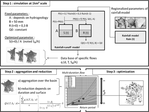
The first step is to generate specific flow quantiles for each 1 km² pixel. In this way, independent hourly rainfall events are simulated at each pixel, using regionalized parameters from the rainfall generator. These hourly rainfall events are converted into independent flood events using a simple rainfall–runoff model, in which some parameters are fixed (in part because the model is being used on a 1-km² pixel).

The hydrological model is of the Irstea GR type (www://cemagref.fr/webgr/). It consists of two reservoirs and a unit hydrograph (Arnaud et al. 2011) and is used in event mode to convert the hourly rain scenarios into flood scenarios at pixel scale. After testing the different structures, we selected those that performed the best in the flood modelling of 12 small basins (each about 1 km² area). Thus, we chose to fix most of the model parameters except the first reservoir’s initial recharge level. The model rainfall input first goes through a simple unit hydrograph that distributes the rainfall in two 1-h time steps: 70% in the first time step and 30% in the second. The capacity of the first reservoir A was set as a function of the main hydrogeological classes determined according to the territory (Aubert et al. 2013). The capacity of reservoir B was set at 50 mm (during the summer) and 100 mm (during the winter), and its initial recharge level R at 30% of B’s capacity. Reservoir B is the second routing function after the unit hydrograph for modelling transfer occurring on 1-km² pixels. Reservoir A’s initial recharge level (S₀/A) is therefore the only variable parameter (varying from 0 to 1). Simulations are performed for different S₀/A values; then flood events are simulated for each of those values, at each pixel. The flood quantiles are extracted empirically from these simulated events. Baseflow (Q₀) is added to the generated flows; Q₀ corresponds to the estimate of mean monthly specific flow, obtained using the LOIEAU regional method for estimating water resources (Folton and Lavabre 2006, 2007). While this value is often negligible compared to simulated flood flows, it needs to be factored in when calibrating the method, because it enables the distinction between surface runoff and subsurface runoff, thus avoiding a calibration bias.

The generated flood events are assigned to a simulation period. and analysed empirically to calculate the flood quantile values. Since the number of events per year is known (it is one of the rainfall model parameters), there is a correspondence between the empirical frequency and the return period (in year). The flood quantiles are read directly from the empirical distribution for return periods that are 100-times shorter than the simulation period to ensure the stability of the empirical frequencies. For example, to obtain millenial quantiles, the equivalent of 100 000 years of rainfall events is simulated and the 1000-year quantiles are estimated by the 100th highest value. This task is performed for each of the 550 000 pixels that cover metropolitan France. The spatial variability of specific flows for a same duration, a same return period and a same S₀/A value is mainly caused by the variability of simulated rainfall, then by the size of reservoir A, and finally, to a lesser extent, by the baseflow Q₀. The second step is to calculate the flood quantiles at gauged catchment outlets for different S₀/A parameter values. For each catchment and each S₀/A value, the runoff on catchment pixels is cumulated. This value is then reduced by a function that depends on catchment surface area and mean flow duration (Fouchier 2010, Aubert 2012). This function allows factoring in areal reduction of rainfall and flood routing simultaneously. It is represented by equations (1) and (2):

(1)

(2)

with the terms and

where n is the number of 1-km² pixels contained on the catchment; S is catchment area in km²; Q(d,T,S₀/A) is mean flow (of duration d and return period T) calculated at the catchment outlet (d = 0 for peak flow) for a given S₀/A value; is the mean flow of duration d and return period T, simulated for a catchment pixel (d = 0 for peak flow) for a given S₀/A value. Parameters α₁, α₂, β_1, β₂, ɣ₁ and ɣ₂ are assumed constant over metropolitan France and were calibrated in a preliminary study with calibration data. This study showed that calibration period does not influence the parameter’s value estimated over the French territory and α₁, α₂, β₁, β₂, ɣ₁ and ɣ₂ values are fixed. In this way the flows are obtained for each catchment.

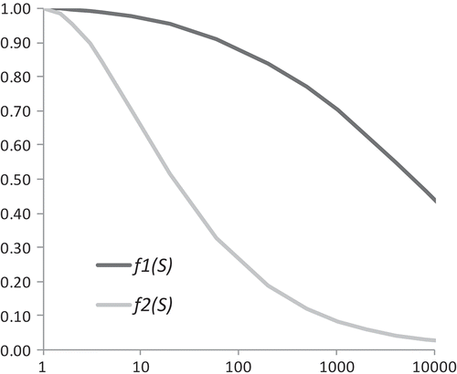
The areal reduction factor is modelled by the functions and presented in Fig. 2, where represents areal reduction of flow averaged over more than 24 h, and represents areal reduction of the difference between flow average over less than 24 h and flow averaged on 24 h.

Figure 2. Representation of the areal reduction function.

The third step is the actual calibration of the method and consists of finding the value that minimizes the deviations between the six quantiles obtained from observations (peak flows and mean daily runoff for 2-, 5- and 10-year return periods) and the same six quantiles provided by the SHYREG method. The quantiles from observations are estimated by fitting a GEV probability distribution for which the value of the shape parameter is imposed between 0 and 0.4. The choice of probability distribution is relatively insignificant as long as you are dealing with observated frequencies (T < 10 years). For each gauged catchment, then, the SHYREG method can be calibrated by optimizing a single parameter, on which the regionalization process will rely to apply the method over the entire drainage network (including ungauged environments).

Setting local parameters concerns only the rainfall yield (production), via the calibration of the S₀/A parameter. When it is calibrated, this parameter also allows us to offset the assumptions made about the other parameters (fixed or regional parameter) which have been set. Since this is not a continuous method, we assumed that the rainfall events, which are generated independently, always occur in a system where the initial state is the same, and are given by the parameter S₀/A.

3 Flow data and assessment index

3.1 The data

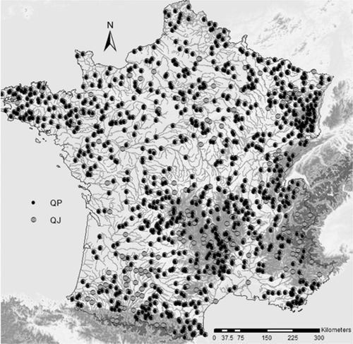
Even if the SHYREG method was designed as a multivariate approach, the present study focuses on only two flood characteristics: peak flow and daily runoff. The data analysed are runoff series recorded at 1172 gauging stations in metropolitan France for which catchment areas range from 10 to 2000 km². While these series are available in daily time steps, only 605 of them also provide instantaneous runoff series, which are usually observed over shorter periods. These stations, shown in Fig. 3, were chosen within the framework of the ANR ExtraFlo² project, from the national Hydro database for the most part, but also from database of Electricité de France (16 stations). They were chosen for their rating curve quality (high level of water deemed satisfactory by the observation manager) and for their observation period (long enough to provide significant statistics: more than 20 years for all stations, with a median of 40 years). Highly specific stations (heavily karstic or anthropized catchments) were excluded (Organde et al. 2013). Some of the station selection criteria are based on tests, like trends and step-changes tests, defined in Renard et al. (2008).

Figure 3. Locations of the catchment outlets studied, with grey points showing daily time steps (QJ) only and black points showing instantaneous time steps (QP).

3.2 Assessment index

The framework developed for the ANR ExtraFlo project was used to assess the SHYREG method. This framework defines a decomposition strategy to differentiate between the calibration (training set) and validation (testing set) periods described in the following paragraph. It also defines the indices used to assess the methods’ results. A thorough description of this assessment platform is given in Renard et al. (2013).

This study briefly describes some of these indices that were used to assess method reliability and stability.

Two performance indices are designed to evaluate the goodness-of-fit with particular care for the extreme part of the distribution. These indices allow us to judge the reliability of a given method on a whole territory, assessing the ability of a model to assign correct exceedence probabilities for several stations. These indices (Fig. 4 shows how these are determined) are:

• NT is based on the number of quantile excesses: it verifies whether the number of observations above a T-year quantile estimated by a given method is consistent with the empirical quantile level. The theoretical distribution of said number of observations is then identified by a binomial distribution for parameters n (number of years of observation) and 1/T (annual frequency of success) (Renard et al. 2013).

• FF is used, e.g. by England et al. (2003) and Garavaglia et al. (2011) and corresponds to the frequency a method gives for the highest observed value in n years of observation. Under the reliability assumption, the theoretical distribution of this index is characterized by a Beta(n,1) distribution with parameter n (number of years of observation) (Kumaraswamy 1980).

Figure 4. Calculation principle for reliability indices NT and FF.

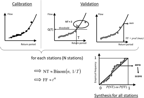
First the method is calibrated on the observations from the calibration set (black curves and black dots in Fig. 4). The values for NT and FF are then calculated based on the observations in the validation set (grey dots). By inverting the theoretical probability distributions for these indices (binomial for NT and beta for FF), their probabilities of occurrence are obtained, P(NT) and P(FF), which should follow a uniform probability if the model is reliable. The reliability of the methods is determined by the deviation between the observed probability and the theoretical probability for NT and FF (the graph at the bottom of Fig. 4). If the frequency distributions for P(NT) and P(FF) align around the bisector − i.e. close to a uniform law − then the method has no systematic bias. Graphical analysis shows the nature of the biases of the method. If the distribution is below the bisecting line, then the method tends to underestimate flood quantiles, whereas if it is above, the method tends to overestimate flood quantiles on the studied territory. When the distribution appears as an S-shaped curve, it means that the method is over-parameterized.

The stability of a frequency analysis method is linked to its ability to produce similar results when it is calibrated on different samples. To determine the stability of a method, a model calibration is performed independently on two different data samples (C1 and C2) leading to two quantile estimations (). Then the relative deviations between the quantiles for different return periods (T) and at each site (i) can be estimated (equation (3)) (Garavaglia et al. 2011):

(3)

A stable method is then characterized by a value of SPAN close to 0.

The graphical analysis of the different indices can be synthesized by calculating scores, which are based on calculations of the area between the observed distribution and the theoretical distribution (bisecting line) for each index (Fig. 4). By standardizing this area, it is possible to make all scores vary between 0 (poor performance) and 1 (perfect performance) (Renard et al. 2013).

3.3 Decomposition

To assess the method’s performance, statistical decomposition was performed on the observation years. For method reliability, the observation years were split into two samples: a calibration sample consisting of a random sampling of the years used to calibrate the method, and a validation sample composed of the rest of the years. For reliability, three decompositions were performed:

• C50V50: out of 519 daily runoff series (and of 605 instantaneous runoff series) with at least 40 years (respectively, 20 years) of observations, 50% of the years were used for calibration and 50% years were used for validation;

• C33V66: out of 519 daily runoff series (and of 605 instantaneous runoff series) with at least 40 years (respectively, 20 years) of observations, 33% of the years were used for calibration and 66% years were used for validation

• CVrecord: out of 1143 stations with at least 15 years of data, calibration was performed on the complete series without the year of record, and validation was performed on the complete series including the year of record (in this case, it is not a random sampling).

For method stability, the years were decomposed into two calibration sub-samples having the same size:

• calibration sub-sample 1 (C1), the years on which the method was calibrated; and

• calibration sub-sample 2 (C2), with the same sample size as C1, also used to calibrate the method.

Because method stability could depend on the amount of data available, decomposition was performed several times using the same sample size over 10, 15 and 20 years. The decomposition sets were labelled CC_10, CC_15, and CC_20, respectively, and required gauging stations with minimum observation periods of 20, 30 and 40 years, respectively. Due to the lengths of the runoff series, decomposition was performed only on daily data for which the observation periods were longer. On this basis, the number of available stations was 1122 stations with more than 20 years of data, 848 stations with more than 30 years of data, and 432 stations with more than 40 years of data.

4 Results

The performance of the SHYREG method was analysed by viewing the frequency distributions for P(NT) and P(FF) and stability index SPAN and computing the corresponding scores (indicated in the graph legend). To put the results of the SHYREG method into perspective, we compared these results to those obtained with two other statistical models commonly used in France: the Gumbel distribution (two parameters) and the GEV distribution (three parameters), for which the parameters are estimated by the L-moments method. This comparison is far from being exhaustive, and serves only to put the results into perspective compared to simple, well-known methods. First we present the results for daily flow estimates.

4.1 Reliability of the method

To judge the method’s reliability FF and NT were used. The NT was calculated for 10- and 100-year return periods (values N10 and N100). The graphs in Fig. 5 show the index frequency distributions for the three models that were compared (SHYREG, Gumbel distribution and GEV distribution), obtained at the C50V50 decomposition validation stations. The index for each curve is indicated in the upper left-hand corner.

Figure 5. Frequency distribution for (a) P(FF), (b) P(N10) and (c) P(N100).

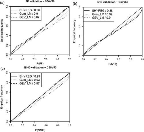
The values of FF and N100 represent the capacity of the models to assign accurate frequencies to extreme values, while the value of N10 determines the ability to exceed rare values. In the case of extreme values, the values of SHYREG’s reliability index are very good. The two statistical models also perform well. The frequency distribution analysis of P(FF), however, reveals a tendency of the purely statistical models to underestimate the frequency of the highest records in some cases (curve below the bisecting line). Assigning a P(FF) of 1 is particularly problematic, since the record observed over the validation period is deemed ‘improbable’. This was the case for 19 stations out of the 519 analysed, when calibrating a GEV distribution based on the calibration sample. The GEV distribution has three calibration parameters, so it can be calibrated as closely as possible to the empirical distribution (and presents the risk of over-fitting). If the empirical distribution has no extreme values, it is likely that the proposed extrapolation will underestimate the probability of observing a high value. The extrapolation to rare frequencies proposed by the SHYREG method, on the other hand, is linked directly to the extrapolation proposed by the rainfall model, in combination with the rainfall–runoff model’s saturation capacity. This characteristic seems preferable in proposing a more reliable extrapolation to extreme values.

4.2 Stability of the method

Method stability was determined by analysing the distribution of the index SPAN, estimated from the quantiles for the 10-, 100- and 1,000-year return periods (SPAN10, SPAN100 and SPAN1000). The graphs in Fig. 6 show the results obtained using two 20-year calibration periods (decomposition CC_20).

Figure 6. Frequency distribution for index SPAN computed from the quantiles for (a) 10-year, (b) 100-year and (c) 1000-year return periods.

The methods are generally less stable when dealing with the longest return periods. The instability is even greater for the methods that are calibrated using a larger number of parameters. For instance, fitting a GEV distribution (three parameters) is less stable than fitting a Gumbel distribution (two parameters). For the SHYREG method, fitting the method at site relies only on the calibration of a single parameter that represents catchment production in a simplified way. It is clearly representative of average catchment behaviour and will be weakly influenced by the calibration sample. This is also why calibrating this parameter is based on fit of current flood quantiles (T = 2, 5 and 10 years). The extrapolation stability is then linked to the stability of both the rainfall generator and the rainfall–runoff relationship. Rainfall generator stability was also analysed under the ANR ExtraFlo project. The stability of the SHYREG method’s rainfall generator was shown to be especially stable (Carreau et al. 2013), in agreement with the results of (Muller et al. 2009) showing that the confidence intervals for the quantiles provided by the hourly rainfall generator are relatively narrow.

4.3 Sampling effect

The performance of the SHYREG method was analysed with respect to the size of period sampling. The reliability is compared on the C33V66, C50V50 and CVrecord decompositions presented in Section 3.3. The stability is tested on decompositions CC_10, CC_15 and CC_20 to analyse the impact of calibration sample size on the method’s stability. To put these results into perspective, we present only the results obtained with Gumbel distribution fit. The choice of Gumbel distribution was motivated by its better stability compared to that of GEV distribution and so, more challenging.

Graph (a) in Fig. 7 shows that the SHYREG method is not highly sensitive to the sampling period. However, we must remember that, in the case of the C33V66 decomposition, we have at least 13 years of calibration. The most interesting result is that the method has a very good reliability index even if the highest value is systematically omitted from the calibration sample. The absence of such a record value in the calibration sample does not create a bias in the SHYREG method’s extreme value estimates. This is particularly significant given the problems that can occur with measurement of extreme flood data. Analysis of graph (b) in Fig. 7 shows that a two-parameter distribution is much more sensitive to sampling, in particular when the highest value is omitted from the sample. In that case, the model almost systematically underestimates the probability of extreme flood occurrence. SHYREG provides more ‘predictive’ extrapolations. This is linked to the method’s heavy reliance on regional rainfall data. Since the rainfall–runoff relationship is not highly sensitive to knowledge of an extreme event (the rainfall–runoff model must be parameterized independently of rainfall), the method has the capability to calibrate itself correctly despite the absence of extreme values in the calibration sample. This is not the case for a method that uses only runoff data, especially if it is calibrated at site and if it has a lot of parameters. That is why methods that use only runoff must factor in regional runoff data (Darlymple 1960, Hosking and Wallis 1997, Ribatet et al. 2007, Ouarda et al. 2008).

Figure 7. Sampling effect on the SHYREG method performance and comparison with that of a Gumbel distribution.

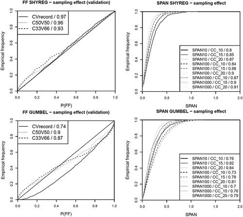
The sampling effect on stability is logical. Graphs (c) and (d) in Fig. 7 show that longer the calibration period, the greater the stability. The length of the calibration period has no real impact on the SHYREG method, whatever the return period. For a Gumbel distribution, stability decreases when the return period increases and when the calibration period decreases. These results are even more marked with the three-parameter distribution GEV.

4.4 Multivariate approach

The SHYREG method is a multivariate method. For the same calibration and simulation, it provides flood quantiles for different durations from peak flow to 3-day flood volumes. The radar charts in Fig. 8 summarize the scores obtained with both daily flows (QJ) and peak flows (QP). The outer-most curves show the best performance.

Figure 8. Performance scores for daily flow (QJ) and peak flow (QP) estimates.

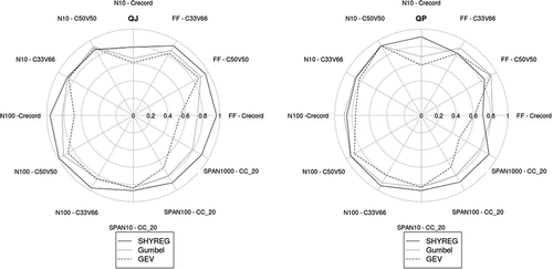
For peak flows, the observations of mean daily flows remain valid. However, there is a slight decrease in SHYREG performance for reliability criteria estimates, because the method slightly overestimates (by roughly 5–10%). The method shows the same stability characteristics. The peak-flow results for a statistical distribution (Gumbel or GEV) are similar to those for daily flows.

The results obtained here show that the method performs well with respect to its capacity to estimate flood quantiles for different durations. This is especially noteworthy because the performance of multivariate approaches tends not to be as good as that of univariate approaches where the parameters can be calibrated for each variable of interest (Gräler et al. 2013).

4.5 Sensitivity to the modelling hypothesis

The stability characteristics of the SHYREG method are linked to the fact that the rainfall–runoff model has few parameters. Calibrating the method relies on a single parameter, S₀/A. The other parameters used in rainfall–runoff models are either fixed values, or regional parameters that are prescribed by the method’s modelling hypotheses and therefore not considered as at-site fitting parameters. To see the impact of modelling hypotheses on the results, different model versions are tested. To avoid overloading the analysis, we present only the tests with a potential impact on the method’s asymptotic behaviour. These tests involve the parameters associated with the method’s equifinality issues as presented by Aubert (2012) and Aubert et al. (2013).

Table 1 lists the hypotheses that were tested for the regionally estimated parameters. In particular, the parameterization of the production reservoir A, which can influence the asymptotic behaviour of the method towards extreme values, is discussed.

• Value of reservoir A In one version of the approach, the maximum capacity of production reservoir A was parameterized as a function of the 100-year daily rainfall (PJ100 in mm) (Organde et al. 2013). This value was optimized for each catchment on data of calibration years and a link with the hydrogeology was established. The value of reservoir A was then regionalized as a function of the hydrogeology. This process is only weakly influenced by station sampling, because the hydrogeology link is relatively weak and serves only to establish key value classes according to hydrogeologically homogeneous regions. Still, it does help to enhance the method’s performance, in particular on catchments in Northern France (Aubert 2012) with high retention capacity.

• Drainage of reservoir A There is no drainage of reservoir A, and this could result in its saturation during an event. A version taking drainage into account was tested, with drainage parameterized as being proportional to the capacity of A (Organde et al. 2013). This relation avoids regionalizing an additional parameter.

• Factoring in baseflow Q₀ The method did not initially take baseflow into account. When the method was adapted to a wider range of hydrological conditions, baseflow was factored in to improve method calibration. Improvements were subsequently observed, especially on catchments that are heavily influenced by subsurface exchange and snow melt (Aubert 2012).

Table 1. Summary of hypotheses tested for regional parameters of rainfall–runoff model.

Test	Value of A	Drainage of A	Q0
Final	Hydrogeology dependent	No drainage	Factored in
Variant 1	Max (200 mm, PJ100)	No drainage	Factored in
Variant 2	Max (200 mm, PJ100)	With drainage	Factored in
Variant 3	Max (200 mm, PJ100)	With drainage	Not factored in Q0 = 0

The radar charts in Fig. 9 provide a synthesis of the SHYREG method’s scores as a function of the different rainfall–runoff modelling hypotheses.

Figure 9. Performance of the SHYREG method for different rainfall–runoff modelling hypotheses used in the method.

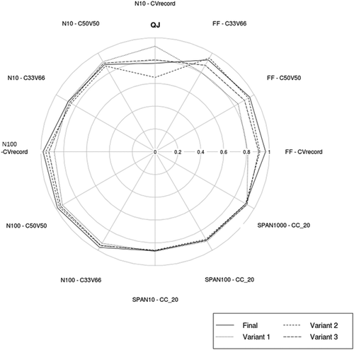
The modelling hypotheses have a moderate impact on the SHYREG model’s performance. The impact mainly concerns the extreme values, seen through the evolution of the FF score. The N10 and N100 values are less sensitive to the modelling hypotheses. However, the method’s stability does not change whatever the hypothesis made. The method’s calibration parameter S₀/A takes on different ‘optimal’ values as a function of the hypotheses tested on the rainfall–runoff model’s production. These values serve to provide identical estimates for the common values (T < 10 years) used to calibrate the model. Conversely, extrapolations to extreme values can be more variable, although certain configurations can compensate. For instance, Variant 2 is able to reach the performance of the Final model by introducing a drainage process into the production reservoir. Variant 1 resulted in a smaller average capacity for reservoir A than the initial model, causing the reservoir to saturate more rapidly. Adding a drainage process helps compensate for the saturation. Variant 3 serves to confirm the advantage of taking into account an initial flow, even if the gain is relatively small. So here, we are verifying that SHYREG’s chosen modelling hypotheses have no impact on the method’s stability, and a relatively small impact on its reliability.

5 Discussion

It is difficult to validate flood frequency analysis methods at only one station, due to the lack of observation data on extreme values. The original methodology used in this study allows the methods to be assessed by compiling statistics over a large number of stations. Comparison with other standard hydrological approaches (fitting a probability distribution on annual maximum flows) also helps to put into perspective the performance of the SHYREG method. The methods are first assessed for their reliability. If the values of the reliability indices are weak then the method is unreliable, because of systematic biases, for example. If the reliability criteria are good, you cannot affirm that the method is reliable but only that it is not incorrect. This is because the criteria cannot detect random biases in a method (only systematic biases). So, in the case of random biases, good reliability values can be due to hazard. However, a method containing this type of random bias will be detected by its poor stability performance.

The SHYREG method has good reliability criteria. Among methods with good reliability criteria, the method with the greatest stability is preferred. This is also the case for the SHYREG method, where the good stability characteristics are due to the small number of parameters (only one parameter) it requires and the type of approach. It would appear that an approach based on rainfall data use leads to particularly relevant flood flow extrapolation.

The SHYREG method was also assessed within the larger framework of the ANR ExtraFlo project, where additional statistical methods, e.g. regional ones, were compared. It emerged that only approaches that take regional data into account can lead to reliability and stability of results close to those of the SHYREG method (Kochanek et al. 2014). The benefits of these RFFA are now emphasized by many authors. These results of the ANR ExtraFlo project showed that the SHYREG method has the same benefits as RFFA.

Despite its good performance, the method needs improvement. In particular, the use of a unique runoff reduction factor for the whole French territory is a strong assumption and needs to be improved in the future. In this way, we are working to impose coefficients for large hydro-climatic areas.

6 Conclusion

This study demonstrates the performance of an extreme flood estimation method by simulation. The SHYREG method is designed to analyse flood flows of all durations (from peak flow to 3-day flood volumes) based on the calibration of a single parameter characterizing catchment production. The SHYREG method was applied to French territory and regionalized; it is currently in operational use to estimate extreme flood flows (Aubert et al. 2013).

Split-sample test procedures were used to assess the method based on its ‘predictive’ performance. Statistical reliability and stability criteria were calculated for different sampling configurations. To put the results into perspective, they were compared with those from standard statistical models in use that are based on parametric probability distributions fitted on peak annual flow data (Gumbel distribution and GEV distribution).

The results show that the SHYREG method is highly stable. The method’s stability is linked to the fact that it relies on the regional statistical features of the data and on a simple rainfall–runoff model. Calibrating the method on a catchment is done using a single parameter. The other parameters are set a priori on a regional basis, independently of the rainfall data that are available for the catchment under consideration.

The method’s reliability indices have very good values, better than those found with the standard statistical methods that were tested. A supplementary study showed that to obtain reliability criteria as good as SHYREG’s, you would need to use a regional statistical distribution (Kochanek et al. 2014). The method’s reliability is linked to the type of approach, which proposes an estimation of extreme flows based on regional extreme rainfall data. This type of rainfall dataset as provided by the method was also found to be reliable and stable (Carreau et al. 2013). It was also demonstrated that the method enables relevant ‘predictive’ estimates, e.g. by assigning correct return periods to the record values missing from the calibration data.

Disclosure statement

No potential conflict of interest was reported by the authors.

Acknowledgements

The HYDRO database (Ministry of environment) and EDF are gratefully acknowledged for providing the data. The authors thank ANR ExtraFlo project members for their contribution to the evaluation framework development.

Additional information

Funding

This work was partially supported by the French Research Agency (ANR) through the project EXTRAFLO (https://extraflo.cemagref.fr/).

Notes

¹ The hourly rainfall generator is calibrated for two seasons: the summer (from June to November) and the winter (from December to May). In this way, we distinguish the long events with low rainfall intensity and the short events characterized by high quantity of rainfall.

² The purpose of the ExtraFlo project (Extreme Rainfall and Floods), funded by the French national research agency ANR, was to establish a comparison framework of methods for estimating extreme rainfall and flood in France.

References

- Arnaud, P., et al., 2008a. Régionalisation d’un générateur de pluies horaires sur la France métropolitaine pour la connaissance de l’aléa pluviographique. Hydrological Sciences Journal, 53 (1), 34–47. doi:10.1623/hysj.53.1.34
- Arnaud, P., et al., 2008b. Regionalization of an hourly rainfall model in French territory for rainfall risk estimation. Hydrological Sciences Journal, 53 (1), 21p.
- Arnaud, P., et al., 2011. Sensitivity of hydrological models to uncertainty in rainfall input. Hydrological Sciences Journal, 56 (3), 397–410. doi:10.1080/02626667.2011.563742
- Arnaud, P., Fine, J.-A., and Lavabre, J., 2007. An hourly rainfall generation model applicable to all types of climate. Atmospheric Research, 85 (2), 230–242. doi:10.1016/j.atmosres.2007.01.002
- Arnaud, P. and Lavabre, J., 1999. Using a stochastic model for generating hourly hyetographs to study extreme rainfalls. Hydrological Sciences Journal, 44 (3), 433–446. doi:10.1080/02626669909492238
- Arnaud, P. and Lavabre, J., 2002. Coupled rainfall model and discharge model for flood frequency estimation. Water Resources Research, 38 (6), 11-1–11-11. doi:10.1029/2001WR000474
- Arnaud, P. and Lavabre, J., 2010. Estimation de l’aléa pluvial en France métropolitaine. QUAE ed. Paris: Update Sciences & Technologies, 158 pages.
- Aubert, Y., 2012. Estimation des valeurs extrêmes de débit par la méthode SHYREG: réflexions sur l’équifinalité dans la modélisation de la transformation pluie en débit. Paris: Université Pierre et Marie Curie.
- Aubert, Y., et al., 2013. La méthode SHYREG débit, application sur 1605 bassins versants en France Métropolitaine. Hydrological Sciences Journal, 59 (5), 993–1005.
- Aubert, Y., et al., 2014. Rainfall frequency analysis using a hourly rainfall model calibrated on weather patterns: application on Reunion Island. In: G.R. Abstracts, ed. EGU General Assembly 2014-7220, Vienna. Germany: Copernicus Publications, 1.
- Blazkova, S. and Beven, K., 2004. Flood frequency estimation by continuous simulation of subcatchment rainfalls and discharges with the aim of improving dam safety assessment in a large basin in the Czech Republic. Journal of Hydrology, 292 (1–4), 153–172. doi:10.1016/j.jhydrol.2003.12.025
- Boughton, W. and Droop, O., 2003. Continuous simulation for design flood estimation—a review. Environmental Modelling and Software, 18 (4), 309–318. doi:10.1016/S1364-8152(03)00004-5
- Cadavid, L., Obeysekera, J.T.B., and Shen, H.W., 1991. Flood‐Frequency Derivation from Kinematic Wave. Journal of Hydraulic Engineering, 117 (4), 489–510. doi:10.1061/(ASCE)0733-9429(1991)117:4(489)
- Cantet, P. and Arnaud, P., 2014. Extreme rainfall analysis by a stochastic model: impact of the copula choice on the sub-daily rainfall generation. Stochastic Environmental Research and Risk Assessment, 28 (6), 1479–1492. doi:10.1007/s00477-014-0852-0
- Cantet, P., Bacro, J.-N., and Arnaud, P., 2011. Using a rainfall stochastic generator to detect trends in extreme rainfall. Stochastic Environmental Research and Risk Assessment, 25 (3), 429–441. doi:10.1007/s00477-010-0440-x
- Carreau, J., et al., 2013. Extreme rainfall analysis at ungauged sites in the South of France: comparison of three approaches. Journal de la Société Française de Statistique, 154 (2), 119–138.
- Castellarin, A., et al., 2012. Review of applied statistical methods for flood frequency analysis in Europe: WG2 of COST Action ES0901. UK: Centre for Ecology & Hydrology.
- Cernesson, F., Lavabre, J., and Masson, J.-M., 1996. Stochastic model for generating hourly hyetographs. Atmospheric Research, 42, 149–161. doi:10.1016/0169-8095(95)00060-7
- Chow, V.T., Maidment, D.R., and Mays, L.W., 1988. Applied hydrology. New York: McGraw-Hill.
- Coles, S., 2001. An introduction to statistical modeling of extreme values. Heidelberg: Springer-Verlag.
- Darlymple, T. 1960. Flood-frequency analysis. US Geological Survey Water Supply Paper 1543A.
- Eagleson, P.S., 1972. Dynamics of flood frequency. Water Resources Research, 8 (4), 878–898. doi:10.1029/WR008i004p00878
- England, J.F., Jarrett, R.D., and Salas, J.D., 2003. Data-based comparisons of moments estimators using historical and paleoflood data. Journal of Hydrology, 278 (1–4), 172–196. doi:10.1016/S0022-1694(03)00141-0
- Folton, N. and Lavabre, J. 2006. Regionalization of a monthly rainfall–runoff model for the southern half of France based on a sample of 880 gauged catchments. In: Andréassian et al., eds. Large sample basin experiments for hydrological model parameterization: Results of the MOdel Parameter EXperiment - MOPEX. Wallingford, UK: International Association of Hydrological Sciences. IAHS Publ. 307, 264–277. Available at: http://iahs.info/uploads/dms/13620.27-264-277-47-FOLTON.pdf
- Folton, N. and Lavabre, J. 2007. Approche par modélisation pluie–débit pour la connaissance régionale de la ressource en eau: application à la moitié du territoire français. La Houille Blanche, n° 03-2007, 64–70.
- Fouchier, C., 2010. Développement d’une méthodologie pour la connaissance régionale des crues. Montpellier: Université Montpellier II Sciences et techniques du Languedoc.
- Garavaglia, F., et al., 2011. Reliability and robustness of rainfall compound distribution model based on weather pattern sub-sampling. Hydrology and Earth System Sciences, 15 (2), 519–532. doi:10.5194/hess-15-519-2011
- Gräler, B., et al., 2013. Multivariate return periods in hydrology: a critical and practical review focusing on synthetic design hydrograph estimation. Hydrology and Earth System Sciences, 17 (4), 1281–1296. doi:10.5194/hess-17-1281-2013
- Guillot, P. and Duband, D. 1967. La méthode du Gradex pour le calcul de la probabilité des crues à partir des pluies. Wallingford, UK: International Association of Hydrological Sciences, IAHS Publ. 84. Available at: http://iahs.info/uploads/dms/084063.pdf
- Hosking, J.R.M. and Wallis, J.R., 1993. Some statistics useful in regional frequency analysis. Water Resources Research, 29 (2), 271–281. doi:10.1029/92WR01980
- Hosking, J.R.M. and Wallis, J.R., 1997. Regional frequency analysis: an approach based on L-moments. Cambridge: Cambridge University Press.
- Javelle, P., et al., 2010. Flash flood warning at ungauged locations using radar rainfall and antecedent soil moisture estimations. Journal of Hydrology, 394 (1–2), 267–274. doi:10.1016/j.jhydrol.2010.03.032
- Katz, R.W., Parlange, M.B., and Naveau, P., 2002. Statistics of extremes in hydrology. Advances in Water Resources, 25 (8–12), 1287–1304. doi:10.1016/S0309-1708(02)00056-8
- Klemeš, V. 1993. Probability of extreme hydrometeorological events – a different approach. In: Extreme hydrological events: Precipitation, floods and droughts, Yokohama. Wallingford, UK: International Association of Hydrological Sciences, IAHS Publ. 213, 167–176.
- Kochanek, K., et al., 2014. A data-base comparison of flood frequency analysis methods used in France. Natural Hazards and Earth System Sciences, 14, 295–308.
- Kumaraswamy, P., 1980. A generalized probability density function for double-bounded random processes. Journal of Hydrology, 46 (1–2), 79–88. doi:10.1016/0022-1694(80)90036-0
- Lang, M. and Lavabre, J., 2007. Estimation de la crue centennale pour la prévention des risques d’inondations. Versailles: Edition Quae.
- Lavabre, J., et al., 2009. Crue de projet ou cote de projet ? Exemple des barrages écrêteurs de crue du département du Gard. ed. Colloque CFBR-SHF: Dimensionnement et fonctionnement des évacuateurs de crues, Lyon, 20-21 janvier 2009.
- Lavabre, J., et al. 2010. Crues de projet ou cotes de projet ? Exemple des barrages écrêteurs de crue du département du Gard. La Houille Blanche, n° 2-2010, 58–64.
- Li, J., et al., 2014. An efficient causative event-based approach for deriving the annual flood frequency distribution. Journal of Hydrology, 510, 412–423. doi:10.1016/j.jhydrol.2013.12.035
- Llamas, J., 1993. Hydrologie générale principes et applications. 2° édition ed. Paris: Gaëtan Morin.
- Margoum, M., et al., 1994. Estimation des crues rares et extrêmes: principes du modèle AGREGEE. Hydrologie Continentale, 9 (1), 85–100.
- Merz, R. and Blöschl, G., 2005. Flood frequency regionalisation—spatial proximity vs. catchment attributes. Journal of Hydrology, 302 (1–4), 283–306. doi:10.1016/j.jhydrol.2004.07.018
- Muller, A., et al., 2009. Uncertainties of extreme rainfall quantiles estimated by a stochastic rainfall model and by a generalized Pareto distribution. Hydrological Sciences Journal, 54 (3), 417–429. doi:10.1623/hysj.54.3.417
- Onof, C., Townend, J., and Kee, R., 2005. Comparison of two hourly to 5-min rainfall disaggregators. Atmospheric Research, 77 (1–4), 176–187. doi:10.1016/j.atmosres.2004.10.022
- Organde, D., et al., 2013. Régionalisation d’une méthode de prédétermination de crue sur l’ensemble du territoire français: la méthode SHYREG. Revue des Sciences de l’Eau, 26 (1), 65–78. doi:10.7202/1014920ar
- Ouarda, T.B.M.J., et al., 2008. Intercomparison of regional flood frequency estimation methods at ungauged sites for a Mexican case study. Journal of Hydrology, 348 (1–2), 40–58. doi:10.1016/j.jhydrol.2007.09.031
- Paquet, E., et al., 2013. The SCHADEX method: A semi-continuous rainfall–runoff simulation for extreme flood estimation. Journal of Hydrology, 495, 23–37. doi:10.1016/j.jhydrol.2013.04.045
- Renard, B., et al., 2008. Regional methods for trend detection: assessing field significance and regional consistency. Water Resources Research, 44 (8), W08419. doi:10.1029/2007WR006268
- Renard, B., et al., 2013. Data-based comparison of frequency analysis methods: A general framework. Water Resources Research, 49 (2), 825–843. doi:10.1002/wrcr.20087
- Ribatet, M., et al., 2007. A regional Bayesian POT model for flood frequency analysis. Stochastic Environmental Research and Risk Assessment, 21 (4), 327–339. doi:10.1007/s00477-006-0068-z
- Shen, H.W., Koch, G.J., and Obeysekera, J.T.B., 1990. Physically based flood features and frequencies. Journal of Hydraulic Engineering, 116 (4), 494–514. doi:10.1061/(ASCE)0733-9429(1990)116:4(494)
- Stedinger, J.R. and Tasker, G.D., 1985. Regional hydrologic analysis: 1. Ordinary, weighted, and generalized least squares compared. Water Resources Research, 21 (9), 1421–1432. doi:10.1029/WR021i009p01421
- Willems, P., et al. 2012. Review of European simulation methods for flood-frequency-estimation. WG3: Flood frequency analysis using rainfall–runoff methods. Report of Cost Action ES0901.