Modelling spatial distribution of surface runoff and sediment yield in a Chinese river basin without continuous sediment monitoring

Abstract

In numerous river basins, continuous data are available for streamflow, but not for sediment transport, soil erosion and sediment yield. Our study shows an approach to assess the spatial distribution of surface runoff and sediment yield in a data-scarce Chinese river basin. Specific objectives of this study were (a) to use the process-based, ecohydrological model SWAT and to parameterize it by fixing as many parameters as possible in advance using field observations, measured data and literature; (b) to calculate streamflow and suspended sediment at the basin outlet as well as surface runoff and sediment yield in each sub-basin using SWAT; and (c) to validate and check the credibility of our simulated results using published literature on land use and associated land management. Our modelling results show a spatial distribution of sediment yield between all 50 sub-basins (0 to 7 t ha^-1 year^-1) with highest amounts predicted for cabbage cultivation (37.5 t ha^-1 year^-1) and only low values for forest (0.2 t ha^-1 year^-1). Previous studies used for validation purposes approve our findings.

Editor Z.W. Kundzewicz; Guest editor V. Krysanova

Résumé

Dans de nombreux bassins versants, des données continues sont disponibles pour le débit, mais pas pour le transport de sédiments, l’érosion du sol et la production de sédiments. Notre étude propose une approche pour évaluer la distribution spatiale du ruissellement et de la production sédimentaire sur un bassin versant chinois disposant de peu de données. Les objectifs spécifiques de cette étude étaient (a) d’utiliser le modèle écohydrologique orienté processus SWAT et de le paramétrer en fixant à l’avance autant de paramètres que possible en utilisant des observations de terrain, des données mesurées et la littérature ; (b) de calculer les débits et les sédiments en suspension à l’exutoire du bassin, ainsi que le ruissellement et la production sédimentaire dans chaque sous-bassin à l’aide de SWAT ; et (c) de valider et de vérifier la crédibilité de nos résultats simulés en utilisant la littérature publiée sur l’occupation du sol et la gestion associée des territoires. Nos résultats de modélisation montrent une distribution spatiale de la production de sédiments sur les 50 sous-bassins (0–7 t ha^-1 an^-1), les plus fortes quantités étant simulées pour la culture du chou (37,5 t ha^-1 an^-1) et les plus faibles pour la forêt (0,2 t ha^-1 an^-1). Des études antérieures utilisées aux fins de validation corroborent nos conclusions.

Key words:

• SWAT
• streamflow
• surface runoff
• sediment
• land use
• China
• Poyang area

Mots clefs:

• SWAT
• débit
• ruissellement
• sédiments
• occupation des sols
• Chine
• région de Poyang

1 INTRODUCTION

Soil erosion is a natural process, but it is worsened globally by human activities, such as agriculture, its expansion and intensification, deforestation and urbanization. Excessive erosion causes problems such as land degradation, desertification, and the siltation of waterways and aquatic ecosystems (Allan et al. 1997). Concerning food security, the productive capacity of cropland is degraded and cropland is lost due to erosion (Lal 2007, Ye and Van Ranst 2009).

China is among the most affected countries in the world in terms of the extent, intensity and economic impact of land degradation. Current estimates suggest that over 40% of the land area (3–4 × 10⁶ km²) is adversely affected by wind and water erosion, loss of grassland, deforestation and salinization. Annual soil loss is around 5 × 10⁹ t and 90% of grassland suffers degradation in the face of rising demand for meat and livestock products (Berry 2003). Yang et al. (2002) classified 3 670 000 km² of the total national area as subject to soil erosion (38.2%), of which 622 200 km² (34.9%) belong to the Yangtze River Basin. Hao et al. (2004) quantified the economic loss stemming from cultivated land degradation in China and differentiated between farmland conversion, desertification, soil erosion and water loss, salinization, soil pollution, reservoir function deterioration, and waterways silting-up.

Factors affecting erosion rates are: precipitation distribution and intensity, topography, slope and slope length, geological formations, soil structure and properties, land use and vegetation cover, as well as land management. Demographic, land-use and climate changes are primary drivers of further soil degradation and loss of cropland (Hill and Peart 1998, Berry 2003, Hao et al. 2004, Chen 2007, Huang et al. 2010).

The spatial distribution and quantification of erosion and sediment discharge are generally known, as are their effects on land surface and water bodies. Nevertheless, there are many regions with insufficient data. The density of hydrological networks, the frequency of the measurements and the type of constituents are limited. In many areas of China, streamflow is measured, but there are no sediment data available. In addition, in some areas there are no studies about soil erosion and sediment input to rivers. Nevertheless, erosion rates can be high in these data-scarce regions and should be regulated. Due to the very high variability of landscape factors and associated terrestrial and aquatic processes, no universal sediment rating curves can be derived. There are many studies that quantify streamflow–sediment relationships (for the Yangtze River: Chen et al. 2001, Zhang et al. 2006, Yang et al. 2007), also dependent on the catchment size, but they neglect the spatial distribution of soil loss from the catchment itself.

The aim of this study is to assess the spatial distribution of surface runoff and sediment yield in a data-scarce catchment in China. This initial study is performed for the Changjiang basin in the Poyang Lake area to establish a solid base for further research and application. Specific objectives of this study were (a) to use the process-based, ecohydrological model SWAT and to parameterize it by fixing as many parameters as possible in advance using field observations, measured data and data from the literature; (b) to calculate streamflow and suspended sediment at the basin outlet as well as surface runoff and sediment yield in each sub-basin using SWAT; and (c) to validate and check the credibility of our simulated results using published literature on land use and associated land management.

2 MATERIALS AND METHODS

2.1 Study area and field investigations

The Poyang Lake basin is located in the central part of the Yangtze River Basin in China. Five major tributaries discharge into the lake: Ganjiang, Xiushui, Fuhe, Raohe and Xinjiang. The study area of the Changjiang is a sub-basin of the Raohe River, with a total area of 6260 km², and lies within the provinces of Jiangxi and Anhui (Fig. 1).

Fig. 1 (a) Location of the study area within the provinces Jiangxi (J) and Anhui (A) in southeastern China; (b) location of the three climate stations (1: Anqing, 2: Jingdezhen, 3: Meilin/Tunxi), and (c) topography (DEM: 90 m SRTM, Jarvis et al. 2008) and river network in the Changjiang River basin, sampling sites (i.e. sub-basin outlets) and the Tankou gauge at the outlet.

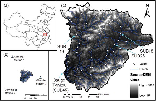
In this study, only the sub-basin of the Changjiang upstream of the Tankou gauging station (29°40ʹ46.92ʹʹN; 117°22ʹ27.15ʹʹE) is considered (Fig. 1). This sub-basin has an area of 1717 km², with mean altitude of 292 m a.s.l., ranging from 57 to 1700 m a.s.l. (SRTM, Jarvis et al. 2008). The landscape is characterized by a hilly terrain with the highest peaks at the northern and northwestern basin borders. The slopes are mild (<5°) in the river valleys, but can be very steep (>50°) in the northwestern mountainous forest areas.

The largest area (approx. 90%) of the basin is located in the administrative county of Qimen in the south of Anhui Province. Only a small part in the southwest of the basin belongs to Fuliang County in Jiangxi Province, and this is where Tankou gauging station is located.

The basin climate is humid subtropical. The average annual temperature is 17.4°C (1971–2000; Jingdezhen Environmental Protection Bureau 2011) and average precipitation is about 1800 mm year^-1 (Jingdezhen Environmental Protection Bureau 2011). From the hydrological point of view, the Southeast Asian monsoon in early summer is most important for the distribution of temporal precipitation. The summer monsoon pattern is characteristic for May–July, with the highest precipitation in the study basin observed during May and June. A belt of moist air masses reaches the study area in early June and results in continuous and heavy rainfalls, often also associated with heavy thunderstorms. In August the catchment is outside of the range of influence of the monsoon front and precipitation is limited to normal amounts for summer monsoon conditions. Towards the end of September, a change in conditions from summer to winter monsoon can be observed, with low temperatures and little precipitation (Domrös and Gongbing 1988). In December and January, precipitation reaches its minimum. From February on, the influence of the winter monsoon weakens, and in March and April the summer monsoon pattern develops again (Zhang and Lin 1992).

The most common soil types are Humic Acrisols (ACu3, 65.7%), Haplic Acrisols (ACh2, 13.8%), Cumulic Anthrosols (ATc1, 10.1%; IIASA Harmonized World Soil Data Base, FAO/IIASA/ISRIC/ISSCAS/JRC 2009). Acrisols which account for 80% of the area, are strongly weathered acid soils with low base saturation and characterized by clay-rich subsoils (FAO 2006).

The land cover is dominated by mixed forest areas. A land-use map was developed for the study area using a supervised multispectral classification approach based on Landsat TM data of the year 2006 (see for details Schmalz et al. 2012). The most important land-use classes are mixed forest (70.0%), arable land (16.7%) and tea plantations (10.8%) (Table 1). Clear-cutting areas of forests were defined as rangeland. Field observations confirm the prevailing cultivation of rice, vegetables and tea in the floodplains and partly on the hillslopes.

Table 1 Relative land-use cover in the Changjiang catchment (using a supervised multispectral classification approach based on Landsat TM data of the year 2006; Schmalz et al. 2012).

Land-use class	Proportion of study area (%)
Mixed forest	70.0
Arable land	16.7
Tea	10.8
Rangeland	2.0
Settlements	0.3
Water	0.2

The total population of the area was about 190 000 in 2009 (Anhui Statistical Bureau 2010). The largest city is Qimen (Anhui Province), but most of the basin is dominated by rural fabric.

Within the study area, 50 points were selected (Fig. 1, Schmalz et al. 2012), distributed over the catchment area with respect to the following criteria: (a) altitude, (b) anthropogenic impact on the sampling site, and (c) stream size. Approximately 40% of the sampling points are located at mountainous stream and river sections, while the remainder lie at lowland rivers. Three classes of anthropogenic pressure were defined: (i) low pressure—no to moderate agriculture and a few small villages, (ii) medium pressure—moderate to extensive agriculture and many small villages, and (iii) high pressure—intensive agriculture and small to large cities (Kuemmerlen et al. 2012). The 50 points were used as sub-basin outlets in the modelling study (see Section 2.3).

Two field campaigns were conducted: in October 2010 and February–March 2011. Detailed investigations were carried out at 12 points: river width, water depth and flow velocity at different verticals and depths (with portable velocity and discharge measurement devices ADC or QLiner from OTT Hydromet GmbH, Kempten, Germany) were measured to calculate the discharge. Water samples were taken and suspended sediment analyses (filtration) conducted at the laboratory of the Institute of Hydrobiology, Chinese Academy of Sciences, Wuhan, China. Furthermore, land use of the surrounding areas was mapped. Due to time limitations, these 12 points were selected to represent lowland and mountain streams with different catchment sizes. The calculated discharge (not shown) and the analysed suspended sediment values gave an indication about the conditions during baseflow conditions and helped during the calibration process, additionally to the long-term discharge values at the outlet (see Section 2.3).

2.2 The SWAT model

The ecohydrological model SWAT (Soil and Water Assessment Tool, Arnold et al. 1998) is a physically-based model system, which uses continuous daily steps. The SWAT model was selected to simulate streamflow, water flow components and sediment yield dynamics at a watershed scale. The simulated watershed can be divided into sub-basins and then further delineated into hydrologic response units (HRUs) representing units of the same slope-soil-land cover combinations.

The necessary input data for the model include a digital elevation model (DEM), soil and land-use maps and their corresponding databases, land management information, climate data, and loadings from wastewater treatment plants.

The simulation of the hydrological processes of a watershed is separated into a land phase and a water or routing phase (Neitsch et al. 2011). The simulation of the land phase is based on the water balance equation, which is calculated separately for each HRU. The hydrological cycle is driven by climatic variables. Processes taken into account include interception, evapotranspiration, infiltration, percolation and recharge, as well as surface runoff, and lateral and return flow. The land phase controls the amount of water, sediment, nutrient and pesticide loadings to the main channel in each sub-basin. Runoff generated in the HRUs is summed up to constitute the amount of water reaching the main channel in each sub-basin. The water or routing phase is defined as the movement of water, sediments, etc. through the channel network to the watershed outlet (Neitsch et al. 2011). The routing of runoff in the channel is specified in the SWAT model by using either the variable storage coefficient method (Williams 1969; used herein), or the Muskingum routing method (Overton 1966).

Sediment yield is estimated for each HRU using the empirical Modified Universal Soil Loss Equation (MUSLE; Williams 1975). The soil erosion load is calculated by using surface runoff volume, peak runoff rate, HRU area, USLE (Universal Soil Loss Equation) soil erodibility factor, USLE cover and management factor, USLE support practice factor, USLE topographic factor and coarse fragment factor. Sediment yield calculated by MUSLE refers to the field erosion. Simulated erosion processes include detachment, transport and deposition of soil particles by the erosive forces of raindrops and surface runoff. Erosion types that can be depicted with the MUSLE are sheet and rill erosion. Sediment routing is controlled by the nature of the sediment (D50), and flow velocity. It is affected by sediment deposition and channel degradation.

2.3 SWAT model set-up, flow calibration and sediment parameterization

For this study, the SWAT model used was version SWAT2009 (Revision 488). The available input data used to drive the hydrological model algorithms were derived from different sources, literature research and field measurements, as presented in Table 2.

Table 2 Data input necessary to depict water and sediment fluxes in the basin.

Data used for the SWAT model	Data source and details
Digital elevation model	SRTM 90 m, Jarvis et al. (2008)
Stream network	Derived from SRTM-DEM with ArcMap, manually corrected (comparison to Google Earth)
Soil map	IIASA Harmonized World Soil Data Base, 800 m, FAO/IIASA/ISRIC/ISSCAS/JRC (2009)
Physical soil parameters	IIASA, ISRIC
Land-use map	90 m, Schmalz et al. (2012)
Vegetation parameters	SWAT database (Neitsch et al. 2011)
Crop management	Farmer interviews (Song 2011) and literature research concerning the dominant crops tea (Ruan et al. 2002), rice (Pan and Shi 2002, Rice Knowledge Bank) and cabbage (AELF, Lattauschke 2006)
Climate data (precipitation, temperature, humidity, wind, solar radiation)	Daily climate data 1960–2010 from the stations Jingdezhen 58527, Meilin/Tunxi 58531, Anqing 58424 (CMA 2011).
Discharge data for calibration	Tankou gauging station (Jiangxi Province): daily discharge data 1981–2010 (Jiangxi Hydrological Bureau 2011)
Suspended sediment concentrations	Field measurements (see Section 2.1)

Sources

AELF (2011).

IIASA: Harmonized World Soil Database. http://www.iiasa.ac.at/Research/LUC/External-World-soil-database/HTML/HWSD_Data.html?sb=4 [Accessed 25 June 2010].

ISRIC (2010).

Rice Knowledge Bank: http://www.knowledgebank.irri.org/rice.htm [Accessed 29 July 2011].

Table 3 Variables used for the calibration of streamflow at Tankou gauging station and their initial and final values. ‘Fixed’ means to have set a fixed value according to literature research or expert knowledge, ‘calculated’ variables are explained with the corresponding procedure in the text, ‘calibrated’ means that the variable was calibrated by manual adjustment and using SWAT-CUP (see text).

Variable name	Definition (Unit)	Initial value	Final value	Input file	Procedure
PET method	Method for calculating potential evapotranspiration		Penman-Monteith	BSN	Fixed
EPCO	Plant evaporation compensation factor	1	0.99	BSN	Calibrated
ESCO	soil evaporation compensation factor	0.95	0.01	BSN	Calibrated
Surlag	Surface runoff lag coefficient	4	0.6	BSN	Calibrated
Alpha-bf	Baseflow alpha factor (d)	0.048	0.0524	GW	Calculated
GW_DELAY	Groundwater delay time (d)	31	44	GW	Calculated
GW-Revap	Groundwater revap coefficient	0.02	0.19	GW	Calibrated
Revapmn	Threshold depth of water in the shallow aquifer for revap to occur (mm)	1	1.875	GW	Calibrated
Rchrg_Dp	Groundwater recharge to deep aquifer (fraction)	0.05	0	GW	Fixed
Alpha-BNK	Baseflow alpha factor for bank storage (d)	0	0.64	RTE	Calibrated
CH_K2	Effective hydraulic conductivity in main channel alluvium (mm h^-1)	0	50	RTE	Fixed based on tables in Arnold et al. (2011)
CH_N2	Manning’s n for the main channel	0.014	0.075	RTE	Fixed based on tables in Arnold et al. (2011)
CANMX FRST	Maximum canopy index	0	20	HRU	Fixed after literature research
CANMX TEA		0	5
CANMX RNGE, RICE, CABG		0	1
CN2 for different land uses	Initial SCS runoff curve number for moisture condition II	31–92; values vary according to land-use class	FRST 57	MGT	Fixed according to Neitsch et al. (2010)
			RICE 86
			CABG 80
			TEA 69
			RNGE 58
			URBN 84
			WATR 92
Mgt operations for different land uses	Agricultural management operations	default	Specific values vary according to crop	MGT	Fixed according to Song (2011) and literature research
GSI FRST	Maximum stomatal conductance at high solar radiation and low vapour pressure deficit (m s^-1)	0.002	0.006	crop.dat	Fixed after literature research
BLAI FRST	Maximum potential leaf area index	5	7	crop.dat	Fixed after literature research
Point source discharge (flow, NO3 and min P)	Estimated waste water entries: water flow, N and P (see text)	0	Specific for each sub-basin	rec*.dat	Calculated for 50 sub-basins

The SWAT model was divided into 50 sub-basins and further into 1905 HRUs. Therefore, in-stream data at the 50 sub-basin outlets and data for the 50 sub-basins and their respective HRUs were provided for a detailed spatial analysis within the basin.

Long-term climate data were available from three climate stations, none of which is located within the study area (Fig. 1, Table 2). They are in the southwest, east and northwest of the study area at a distance between 30 and 60 km. The distance to Tankou gauging station is between 40 and 100 km.

Dams and reservoirs were not implemented in the model set-up. Although some smaller dams and reservoirs were observed during the field campaigns, no definite data about dam height, reservoir operation and year of construction could be obtained.

While tea plantations were classified separately on the land-use map, the arable land was further divided into rice and cabbage fields depending on the slope. The agricultural management schedules and operations—such as tillage or fertilization—were implemented (Table 2) as gathered by literature research and by interviews with Chinese farmers in the study area during our two field campaigns (Song 2011). Song (2011) focused on the main cultivated crops—rice, vegetables and tea—to obtain specific management schedules and operations in the region for tillage, fertilization, planting and harvest. The most important information about rice cultivation was that the farmers harvest only once a year, and not twice as in the past.

To take into account wastewater entries, population equivalent values were estimated from the percentage of urban land-use class from each sub-basin (land-use map), as well as the number of inhabitants and the number of enterprises according to the statistical yearbook (Anhui Statistical Bureau 2010). The pollutants entries were calculated with the help of reference values for daily human excreta. As a result, point source discharge for flow, nitrogen and phosphorus could be implemented for each of the 50 sub-basins.

The SWAT model was run for daily time steps. The simulation covers the period 1981–2010, and this is divided into 5-year warm-up (1981–1985), 10-year calibration (2001–2010) and 15-year validation (1986–2000) periods. The calibration period was chosen around the same time at which the satellite image (2006) was taken for deriving the land-use map.

For streamflow calibration and validation, runoff data of Tankou gauging station (Jiangxi Province) are available in a daily time step for the period 1981–2010 (Jiangxi Hydrological Bureau 2011).

Before calibrating the streamflow, it was our intention to calculate and/or fix as many parameters as possible in advance (Table 3):

A baseflow filter program (Arnold et al. 1995, Arnold and Allen 1999) was used to separate baseflow and groundwater recharge from streamflow records. Therefore, the groundwater parameters Alpha-bf (baseflow alpha factor) and GW_DELAY (groundwater delay time) were calculated and used in the calibration procedure (Table 3).

Another focus was on the adaptation of the vegetation variables to the sub-tropical climate conditions in the Chinese study basin. The maximum canopy index (CANMX) was adapted for forest and crops, the maximum stomatal conductance (GSI), as well as the maximum potential leaf area index (BLAI) for the mixed-forest (Table 3). Furthermore, plant parameters for tea were added to the crop database in SWAT (based on Bieger et al. 2012).

Further variables, e.g. SCS runoff curve number, or agricultural management operations, were fixed using values according to literature or expert knowledge (see Table 3).

For the remaining parameters (Table 3), calibration of streamflow was performed manually, and with the help of SWAT-CUP (Abbaspour 2007) using the SUFI-2 (sequential uncertainty fitting) program. This procedure included parameters from the basin, groundwater, and the channel routing input files. The calibrated parameters with their initial and final values are listed in Table 3.

Due to missing measured sediment time series, sediment parameterization was performed without proper sediment calibration and validation; the variables were adjusted manually. The parameter values were estimated as correctly as possible, to reflect the processes in the area. They were compared with field observations within the entire catchment, measured data at the 12 points and the literature. For this study, it was more important to represent the field observations and the processes in the catchment than to perform an auto-calibration with possibly better model performance. The variables used for the sediment parameterization and their final values are listed in Table 4.

Table 4 Variables used for the parameterization of sediment and their initial and final values.

Variable name	Definition (Unit)	Initial value	Final value	Input file
CH_BED_D50	D50 median particle size diameter of channel bed sediment (µm)	500	2000	RTE
PRF	Peak rate adjustment factor for sediment routing in the main channel	1	0.5	BSN
FILTERW	Width of edge-of-field filter strip (m)	0	5	MGT
USLE_C for Cabbage in arable land class	Minimum value of USLE C factor for water erosion applicable to the land cover/plant	0.2	0.05	Crop.dat
USLE_P for CABG	USLE equation support practice factor	1	0.3	MGT
USLE_P for RICE		1	0.1
USLE_P for TEAT		1	0.5

The following three parameters were set with regard to the observations during the field campaigns and were not auto-calibrated. The D50 median particle size diameter of channel bed sediment (CH_BED_D50) was changed according to the substrate investigations in the field. The field observations indicated coarser bed sediment than the SWAT default value. The peak rate adjustment factor for sediment routing in the main channel (PRF) is a variable which influences channel degradation (Arnold et al. 2011). Due to the field sediment investigations observing sediment degradation and deposition, we reduced the value to 0.5. The width of edge-of-field filter strips (FILTERW) was set to 5 m. As with the previous two parameters, it is difficult to set one parameter for the entire basin, or even for each sub-basin or HRU. The distance from agricultural areas to the river varies from zero—cultivation directly at the stream bank—to a long distance. According to the field observations, 5 m is a reasonable mean value.

Two of the USLE equation factors were also changed from the default values. The minimum value of the factor for water erosion applicable to the land cover/plant (USLE_C) for cabbage in the arable land-use class was reduced to that selected by Schönbrodt et al. (2010), which represents a mean value for the Xiangxi catchment. The USLE equation support practice factor (USLE_P) was reduced for cabbage, rice, tea and urban area (Table 4). Field observations confirmed that erosion protection measures were carried out, e.g. bunds surrounding the rice fields, terraces for the cultivation of cabbage.

2.4 SWAT model evaluation

Hydrographs of observed and simulated daily streamflow at Tankou gauging station were used for model evaluation. Furthermore, a number of statistical indices were used to evaluate the model performance, such as the Nash-Sutcliffe efficiency (NSE; Nash and Sutcliffe 1970), the coefficient of determination (r²; Yule 1899), and the percent bias (PBIAS; Gupta et al. 1999). Even though streamflow was calibrated against daily observed data, monthly statistics were calculated to evaluate the model performance according to the general performance ratings proposed by Moriasi et al. (2007) for a monthly time step.

Two further measures were used to assess the goodness of calibration: a p factor and an r factor were calculated by the conducted uncertainty analysis (SUFI-2). The p factor is the percentage of measured data bracketed by the 95% prediction uncertainty (95PPU) and quantifies the degree to which all uncertainties are accounted for. The r factor quantifies the strength of the calibration and is the average thickness of the 95PPU band divided by the standard deviation of the measured data. A p factor of 1 and an r factor of 0 would represent a simulation that exactly corresponds to measured data (Abbaspour 2007).

In addition to the time series analysis of the daily streamflow at the gauging station at the basin outlet, water balance and spatially distributed analyses of flow components were conducted and checked for plausibility.

2.5 Validation of the sediment model results

Previous studies conducted in China analysed erosion processes and sediment yield, some of which used experimental fields or plot studies, others catchment-scale and modelling studies, as summarized in Tables 5–7. Figure 2 shows the location of sediment study areas in China, giving an indication of distances, or differences between the study area and other studies. These studies give an initial overview of the processes in such areas and help in setting the SWAT model parameters. Most importantly, the results from these studies were compared to our model results for validation purposes. Because there are no measured long-term sediment data, we need a validation of our model results derived from these other studies. We used their investigated relationships between land use and sediment yield and transferred these findings and parameter ranges to our results.

Table 5 Studies analysing surface runoff depending on land use.

Reference	Catchment or plots	Method, studied land use, period	Results
El Kateb et al. (2013)	Shaanxi Province (hilly topo-graphy, yellow-brown soil)	Field experiments, 33 erosion plots (7 m^2), five vegetation covers (e.g. tea, forest) and three levels of slope gradient, 15 July–30 October 2008	Runoff was associated with rainfall intensity, vegetation cover and slope gradients
			Ranking: forest < grassland < farmland
			No significant difference between the two forest types (mean: 17–35 m^3 ha^-1), even with different slopes
			Tea plantation: 83 m^3 ha^-1 (slight slope)–190 m^3 ha^-1 (steep slope)
			Proportions of generated runoff (%): 6.6% (moderate slope)–24.5% (steep slope) at tea plantation and 10.7% (moderate slope)−13.0% (slight slope) at the forest (both types), with a rainfall intensity ≤5 mm h^-1; 13.6% (slight slope)–30.5% (steep slope) at the tea plantation and 2.4% (slight slope)–2.9% (steep slope) at the forest (both types), with a rainfall intensity >5 mm h^-1
			For the rainfall event with the highest intensity of 97.5 mm h^-1: highest runoff at tea plantation (104.9 m^3 ha^-1), followed by agriculture (maize, without slopes >30°), then grassland, and lastly forest
Hill and Peart (1998)	Southern China	Review of plot studies, forest, tea, rice	Forest and woodland: 13–99 mm
			Rubber/tea: 13–206 mm
			Upland rice: 3395 mm
			Cultivation on slopes: 1104 mm
			Water yields from cultivated land mostly two orders of magnitude higher than from forest
			Ranking: forest ± woodland < scrub ± grass < tree crops and bare soil < cultivated slopes
Lee et al. (2010)	Korean mountainous area (10 and 17% slope)	Field experiments, rainfall event with 280 mm, Chinese cabbage	286–1167 m^3 ha^-1 (comparing conventional tillage, reduced tillage and reduced tillage with rye mulching)
			Runoff as % of total rainfall amount: 30.6–41.7% (conventional tillage), 15.3–32.9% (reduced tillage), 10.2–21.3% (reduced tillage with rye mulching)
			Conclusion: reduced tillage lowered runoff, increasing surface coverage by rye mulching reduces raindrop impacts, and reduces water flow through rills
Liang et al. (2013)	Taihu Lake area	Rice	Using AWD (alternate wetting and drying) irrigation as a water saving practice minimized surface runoff
			Reduced floodwater depths in the rice fields helped to buffer against runoff events after heavy storms
			Consequently, the number of runoff events and total volume surface runoff was significantly lower
Lu et al. (2004)	Seven plots in Zheijiang Province (red soil region)	Plot study, forest, tea	Differences in runoff mainly determined by vegetation coverage and plant characteristics the deciduous broad-leaf forest showed high adaptability to the red soils and was effective in reducing surface runoff
			Extensive cultivated tea trees had limited growth, so limited water and soil conservation
			Sparse coniferous forest resulted in high runoff (much less than on bare soil)
			Coefficients of runoff: broad-leaf forest < mixed forest < grass land < citrus orchard < tea brush < sparse coniferous forest < bare soil
Wu et al. (2011)	Watershed of Qingshan Lake, Zhejiang Province (yellow red soils)	Field experiments, Chinese cabbage (5 growth stages), 10 simulated rainfalls	Runoff occurrence time decreased with the growth of Chinese cabbage because of the increasing vegetation coverage ratio
			Runoff volumes at seedling and rosette stages were both higher than those at folding stages
			Larger vegetation coverage ratios speeded up the runoff occurrence but did not increase the runoff volumes significantly (growing plant roots hold up surface runoff and leaves intercept rainfall through its special folded formation)
			Folding stages had larger vegetation cover than seedling and rosette stages, which could slow down the surface runoff speed

Table 6 Studies analysing the spatial distribution of sediment yield between sub-basins. See Fig. 2 for catchment locations.

Reference	Catchment	Study aim and period	Method	Results
1. Bieger et al. (2013)	Xiangxi Catchment Three Gorges area of the Hubei Province	Average annual sediment yield, 1981–1993	SWAT model	1987: 0.03–2.56 t ha^-1 year^-1
				2007: soil erosion (47.7%) and sediment loads (41.9%) decreased. Reason: forested area increased by 3.6 % since 1987, large areas of cropland were replaced with orange orchards
2. Li et al. (2010)	Liao watershed of the Poyang Lake area, Jiangxi Province (59% forest)	Annual soil erosion and sediment yield (rain data 1971–2000)	USLE and GIS	Spatial distribution of soil erosion: varies from nil (flat and well-covered areas) to more than 500 t ha-1 year^-1 (mountainous areas with sparse vegetation)
				Average soil erosion: 18.2 t ha^-1 year^-1 (SD: 109.3 t ha^-1 year^-1)
				Erosion rate: 39.5% of the watershed under tolerant erosion, while the rest of the area with erosion to different extents
3. Lu et al. (2003)	Upper Yangtze basin (loess area)	Long-term mean sediment yield, 1957–1987	Interpolation and a mapping approach	Mean: 4.97 t ha^-1 year^-1 (SD 5.19 t ha^-1 year^-1)
				Highest value reached: 31.18 t ha^-1 year^-1
4. Lu et al. (2011)	Poyang Lake basin	Soil erosion for 1990 and 2000	Remote sensing, GIS and USLE	Average soil erosion: 11 t ha^-1 year^-1 (slight)
				Eroded areas mainly located in the Ganjiang and Xinjiang headstreams and in middle reaches and headwaters of the Fuhe and Xiushui Rivers
5. Ouyang et al. (2010)	Longliu watershed, at conjunction of Qinghai–Tibet Plateau and Loess Plateau. Study area is the main part of the Upper Yellow River watershed	Annual soil erosion, simulations of 1977, 1996, 2000 and 2006	SWAT model	Main soil erosion from agricultural land, relatively slight soil erosion in forests and on grassland in steep mountain areas
				Averaged soil erosion loads for the 4-year study period: 9, 10, 7 and 8 t ha^-1 year^-1
				Highest soil erosion loads in the four single years: 160, 81, 85 and 67 t ha^-1 year^-1
6. Shen et al. (2010)	Zhangjiachong watershed (1.62 km^2), Three Gorges Reservoir area	Annual mean soil erosion rate distribution, 2004–2007	Plot measurements, WEPP model	Annual mean soil erosion: 0.2–3.8 t ha^-1 year^-1
				Most serious erosion occurred in regions with intense agricultural activities and where most crops were planted on soil dike terraces
				Least eroded areas were rice paddy fields at low-gradient slopes
7. Wu and Chen (2012)	East River basin (tributary of Pearl River; 25 325 km^2) in southern China	Annual average sediment yield, 1973–1988	SWAT model	Annual average sediment yield: 40.3 t ha^-1 year^-1
				Higher soil erosion rates related to high percentage of agricultural land (~37%)
				Erosion is quite sensitive to soil properties and slope
8. Yan et al. (2011)	Eentire Yangtze basin, and Poyang Lake sub-basin (158 677 km^2)	Sediment yield, 23 years	Based on the sediment monitoring network	Entire Yangtze basin: up to 30 t ha^-1 year^-1
				Poyang Lake sub-basin: 0.75–6.5 t ha^-1 year^-1
				(35 stations; 23 years)

Table 7 Studies analysing the influence of land use on the spatial distribution of sediment yields. See Fig. 2 for catchment locations.

Reference	Catchment	Study aim and period	Method and studied land use	Results
9. Bieger et al. (2012)	Xiangxi Catchment (Three Gorges Area)	Mean annual sediment yield, 1985–1993	SWAT model, crops	48 t ha^-1 year^-1from agricultural areas
10. Chen et al. (2012)	Taiwan	Annual average soil erosion at rice fields (different management), 2005–2007	Experimental study, rice	0.74–4.15 t ha^-1 year^-1
11. El Kateb et al. (2013)	Shaanxi Province	Soil loss, 15 July–30 October 2008	Erosion plots, forest and tea	Highest soil loss: maize and tea
				Tea plantations at slopes >30° were most susceptible to erosion
				Tea plantations generated significantly higher soil loss (1.991–17.552 t ha^-1 year^-1) than forest lands (0.009–0.057 t ha^-1 year^-1) at all the three slope gradients
				Negligible soil losses were generated by forests
				The proportion of the generated soil loss was 7.4–63.5% for tea and 0.13–1.47% for forest
				Forest (cork-oak and pine) did not produce any soil loss until (compared to tea cultivation and grassland) on average, around four times higher runoff was generated
12. Hill and Peart (1998)	Southern China	Mean erosion rates	Review, forest and crops	Forest and woodland: 0.05 t ha^-1 year^-1, cultivated slopes: 62.4 t ha^-1 year^-1
				From cultivated land mostly about three orders of magnitude higher than from forest
13. Huang et al. (2010)	Red soil region at the Ecological Benefit Monitoring Station of the Yangtze River Protection Forest Project, in Hunan Province	Mean annual soil erosion at conventional sloping farmland (maize, peanut, sweet potato, potato, and pumpkin) with three different reforestation types, 2002–2007	Field experiments, forest and crops	Conventional sloping farmland (1.084 t ha^-1 year^-1) > natural succession type forest (0.066 t ha^-1 year^-1) > artificial economic forest (0.059 t ha^-1 year^-1) > pine secondary forest (0.041 t ha^-1 year^-1)
14. Lee et al. (2010)	Korean mountainous area	Soil loss under Chinese cabbage, 280 mm rainfall event	Experimental results, cabbage	Conventional tillage plots: 4.1–11.5 t ha^-1
				Reduced tillage plots: 2.2–2.4 t ha^-1
				Reduced tillage with rye mulching: 0.2–1.3 t ha^-1
				Reduced tillage reduced soil erosion; reduced tillage with rye mulching on soil surface doubled the effect of reducing soil erosion
15. Long et al. (2006)	Zhongjiang, a typical agricultural county of Sichuan Province	Soil erosion, maps of year 2000	GIS spatial analysis, crops	Most serious soil erosion occurred on agricultural land with a slope of 10–25°
				Both farmland and permanent crops were affected by soil erosion, with almost the same soil erosion for corresponding slope conditions
16. RRC AP (2001)	Sri Lanka	Soil erosion in tea plantations	Report; review, tea	0.33 and 250 t ha^-1 year^-1
17. Shen et al. (2010)	Three Gorges Reservoir Area	Soil erosion, sediment loads, 2004–2007	Plot experiments, tea	Tea trees: high soil erosion in the first year; soil stability enhanced gradually with growth
				Hedgerows in the plots reduced sediment loads (mean annual): 39.6%
18. Wang et al. (2013)	Le’an (Raohe basin)	Suspended sediment, June 2010–July 2011, 17 water samples bi-monthly	Suspended sediment monitoring, forest and crops	Suspended sediment concentrations: 0.2–74.4 (average: 9.99 mg L^-1)
				Increasing trend from upstream to downstream
				Northeast area (80% forests and 12% cultivated land): 0.2–40.8 mg L^-1 (average: 6.92 mg L^-1): low, no significant variability
				Southwest area (52% forests and 40% cultivated land): 2.2–74.36 mg L^-1 (average 14.39 mg L^-1): high, varies considerably
				Forests contribute to reduce soil loss and sediment concentration, while arable land and related activities cause considerable soil loss during rainfall events
19. Wu and Chen (2012)	East River Basin	Annual sediment yield, 8-year period	SWAT model, forest and crops	Highest: 409 t ha^-1 year^-1 from the agricultural areas, but for the whole basin 24.9 t ha^-1 year^-1
				105.5 t ha^-1 year^-1 from agricultural land, only 0.2 t ha^-1 year^-1 from forests
20. Zhang et al. (2011a)	Mountainous woodlands in China	Average annual soil loss	USLE, forest	0.0382 t ha^-1 year^-1
				about 99.89% of Chinese woodland area in the slight erosion class, whereas it only resulted in about 41.97% of soil loss under woodland area, and 58.03% of soil loss occurred under high erosion potential zone (>5 t ha^-1 year^-1)
21. Zhang et al. (2011b)	Shangshe catchment of the Dabie Mountains of the Anhui province	Annual soil losses from different land-use types (pine forest, Chinese fir forest, bamboo forest, and tea garden), 2000–2007	Field plot observations, integral equation method, forest and tea	Tea garden: <0.10 t ha^-1, except in 2001 (0.55 t ha^-1), mainly due to the grass cutting and tending
				Chinese fir forest, pine forest and bamboo forest: <0.10 t ha^-1, except: pine forest in 2005 (0.109 t ha^-1)
				bush changed to bare land: soil loss rates of up to 350 t ha^-1
				when vegetation coverage increased to 70 and 80% (natural regeneration), amount of soil erosion decreased significantly to around 3 t ha^-1

Fig. 2 Locations of study areas used for validating sediment model results. Numbers are related to Tables 6 and 7 (missing numbers: 3: Upper Yangtze basin, 8: entire Yangtze basin, 12: southern China, 14: Korean area, 16: area in Sri Lanka, 20: mountainous woodlands). Black circle represents location of study area.

3 RESULTS AND DISCUSSION

3.1 Streamflow and flow components

3.1.1 Streamflow at the basin outlet

The calibration and validation of streamflow at Tankou gauging station show a good fit of simulated and observed data, confirmed by visual comparison of the hydrographs and by the model evaluation statistics (Fig. 3; Table 8). While the values for daily streamflow are NSE = 0.56 and r² = 0.56 (calibration period) and NSE = 0.51 and r² = 0.52 (validation period), the monthly values are much higher at NSE = 0.87 and 0.79, r² = 0.88 and 0.85 in the calibration and validation periods, respectively. According to the general performance ratings proposed by Moriasi et al. (2007), the simulation of streamflow by monthly time steps achieved a very good performance. The uncertainty analysis resulted in a p factor of 0.45 and an r factor of 0.11 after 1500 simulations. These results show a certain weakness of our calibration, as only 45% of the observations are bracketed by the 95PPUs within the narrow prediction interval. However, despite a scarcity of data, the uncertainty is within a reasonable range, the processes are adequately represented and, therefore, the results can be used for further analysis.

Table 8 Model performance for daily and monthly streamflow during calibration and validation periods.

	Calibration 2001–2010	Validation 1986–2000	Calibration 2001–2010	Validation 1986–2000
Time step	Daily	Daily	Monthly	Monthly
NSE	0.56	0.51	0.87	0.79
r^2	0.56	0.52	0.88	0.85
Ave error	−2.69	−7.79	−81.81	−237.13
PBIAS	5.75	12.02	5.75	12.02

Fig. 3 Precipitation, and hydrograph of observed and simulated daily streamflow at Tankou station during the calibration period (2001–2010) (CMA 2011; Jiangxi Hydrological Bureau 2011).

The hydrograph (Fig. 3) shows a seasonal dynamic of high peaks, with flows exceeding 1000 m³ s^-1 during the monsoon period and low flows in winter. When the observed and the simulated streamflow are compared, the general dynamic is recreated quite well, but the simulated curve is smoother than the observed hydrograph with high daily small-scale dynamics. In addition, while the maximum flow volume of most peaks is underestimated, the baseflow during the low-flow periods is slightly overestimated.

The measured data show a distinctive small-scale flow dynamic that cannot be explained by the available climate data from the three climate stations. The simulated streamflow curve reacts as expected to the implemented precipitation distribution. The additional observed small-scale peaks cannot be explained by this. This behaviour might be explained by the regulation of reservoirs, irrigation or industrial facilities, but no such data are available. Therefore, the baseflow of the simulated hydrograph seems to be smoothed.

The lower model performance at a daily time step is probably also due to the implemented precipitation data from three climate stations, none of which is located within the study area (Fig. 1). For modelling, the climate data were spatially distributed on the sub-basins, depending on the distance to the nearest climate station. Therefore, the following spatial distribution resulted for the model set-up: Jingdezhen (southwest) 52.0%, Meilin/Tunxi (east) 43.6%, Anqing (northwest) 4.4%. A comparison of the three climate data sets with each other showed a different rainfall distribution. Even the rainfall events with >100 mm d^-1 show a high degree of variability in magnitude and time, which has a great influence on the runoff. Therefore, correlations were calculated, which show the relationship between precipitation and streamflow (Table 9). It was shown that, on a daily basis, a very low correlation results (r² < 0.26), whereas it is significantly higher on a monthly basis or when three consecutive days were considered. This explains the differences in model performance between daily and monthly resolution.

Table 9 Correlation (r²) between measured precipitation (PCP) and measured streamflow (Q) for the entire simulation period 1986–2010 on daily and monthly basis.

	Q Tankou
	vs PCP Jingdezhen	vs PCP Tunxi	vs PCP Anqing
Daily basis
Entire data set	0.17	0.24	0.07
Monsoon period	0.17	0.26	0.06
Low-flow period	0.09	0.10	0.04
3 days	0.28	0.39	0.18
3 consecutive days
Entire data set	0.28	0.39	0.18
Monthly basis
Entire data set	0.70	0.79	0.59
Monsoon period	0.57	0.73	0.47
Low-flow period	0.49	0.58	0.37

Although in the above-mentioned conditions only monthly time series might be meaningful and result in a better, very good model performance, the daily time step with a satisfactory model performance still shows additionally the temporal variability of streamflow and sediment. It might be possible that, due to the climate input data used, the high streamflow or sediment peaks might be offset somehow, or some peaks are different because of the regional spatial rain pattern. But using these data for further questions as water management or ecological subjects, the dynamics with the full range of possible values is more important than a smoothed monthly curve.

3.1.2 Flow components

3.1.2.1 Flow components at the basin outlet

Considering the outlet of the entire basin at Tankou station, the total water yield was calculated as 799 mm, with the following separated runoff components: surface runoff 265 mm, lateral flow 280 mm and groundwater flow 254 mm (average annual basin values, 2001–2010). Values are different for the floodplains with lowland characteristics among the hilly landscape: surface runoff 242 mm, lateral flow 195 mm and groundwater flow 363 mm (2001–2010; sum 800 mm; sub-basin at the outlet SUB45). The distribution of the components varies seasonally (Fig. 4 for SUB45 at the outlet). There is a distinct maximum from March to July that can be derived from the monsoon precipitation. The very pronounced surface runoff during this period results in erosion processes.

Fig. 4 Flow components within the sub-basin at the basin outlet (site SUB45): values averaged over 10 years (2001–2010, calibration period). Note SUR_Q, surface runoff; LAT_Q, lateral flow; GW_Q, groundwater flow.

We compared these results to analyses from the adjacent Xinjiang catchment. Both catchments are parts of the Poyang lake basin and have similar landscape properties. Altitudes, soils, forest fraction and climate are comparable. The mean annual precipitation is 1878 mm year^-1 (Ye et al. 2011). Only the size of the catchment upstream of Meigang hydrostation is much larger, covering 15 535 km². Ye et al. (2011) calculated that 38% of the measured streamflow was baseflow. Furthermore, Li et al. (2012) estimated that baseflow is 31.3 and 34.5% of total runoff (modelled) for Xinjiang catchment. In our study area of Changjiang, a value of between 0.33 (baseflow Fr2) and 0.50 (baseflow Fr1) was derived for the period 2001–2010. In general, the fraction of water yield contributed by baseflow should fall somewhere between the values for Fr1 and Fr2 (Arnold et al. 1995, Arnold and Allen 1999).

Also for Xinjiang basin, Ye et al. (2011) used the SWAT model to calculate water flow components. Before calibrating the model and considering different soil data, they calculated 718 and 558 mm surface runoff, respectively, which is 35 and 27%, respectively, relating to 2060 mm precipitation (1998–2003). In our Changjiang study, surface runoff was 16% (265 mm) of precipitation (1644 mm). The difference is mostly due to the considerably smaller lateral flow fraction in the Xinjiang study.

3.1.2.2 Surface runoff depending on land use

The flow components in each sub-basin are distributed differently depending on slope, soil and land use. For the entire basin, the highest annual surface runoff was simulated for rice, followed by cabbage. The lowest values appear under forest cover (Table 10 left). This relationship can be confirmed (Table 10 right), as we considered the HRUs with the same soil (ACu3, Humic Acrisol) but different land uses of two example sub-basins: SUB19, a small sub-basin with more mountainous characteristics, and SUB45, the sub-basin at the basin outlet. The mean values between these two sub-basins are similar.

Table 10 Simulated surface runoff (SURQ; average annual values, 2001–2010) (left) for the entire basin depending on land use (LU) and (right) in HRUs of two example sub-basins with different land use and the same soil (LU-Soil). n is the number of HRUs within the selected sub-basin.

LU	SURQ (mm)	SUB	LU-Soil	SURQ mean (mm)	n
Forest	164.82	19	FRST-ACu3	165.50	5
Tea	327.27		TEAT-ACu3	329.19	5
Cabbage	615.87		CABG-ACu3	619.51	4
Rice	702.00		RICE-ACu3	704.61	1
		45	FRST-ACu3	165.84	5
			TEAT-ACu3	335.06	4
			CABG-ACu3	621.98	4
			RICE-ACu3	710.06	1

Hill and Peart (1998) described the same trends in southern China (Table 5), listing surface runoff values based on plot studies for forest and woodland that are a little lower than calculated for this study, but higher values for upland rice and cultivation on slopes (Table 5). The differences can be explained by the fact that rice cultivation in the Changjiang area is mainly allocated to river valleys, with flooded rice paddies. In contrast, upland rice is grown on dry soil. Hill and Peart (1998) mention that the water yields from cultivated land are mostly two orders of magnitude higher than from forest. Calculations for our study show that the relationship of surface runoff between forest and cropland (cabbage) is 1:4. In terms of runoff production, the ranking (low to high) for southern China in Hill and Peart (1998) goes from forest ± woodland, scrub ± grass to tree crops and bare soil, and, finally, cultivated slopes. Our study reveals the following ranking (low to high) for surface runoff: forest – tea – cabbage – rice. Also Lu et al. (2004) reported that the differences in runoff between seven plots in the red soil region were mainly determined by vegetation coverage and plant characteristics. In addition, they differentiated between reduced surface under deciduous broad-leaf forest and high runoff under sparse coniferous forest. The highest runoff was observed on bare soil, which is an indication for our clear-cutting areas (Table 5).

Further studies investigated the occurrence of runoff under coverage of Chinese cabbage. Lee et al. (2010) conducted field experiments in a Korean mountainous area comparing different kinds of tillage. Our modelling study reveals 37% surface runoff of precipitation (average values 2001–2010) under cabbage cultivation with conventional tillage. This is comparable to the values from Lee et al. (2010) (Table 5). Although the position is different, the slopes (10 and 17%) and soils (silty clay loam) are similar. These results can be used for further management planning. Wu et al. (2011) investigated five growth stages of Chinese cabbage (Table 5). Our modelling study does not show such effects of runoff dependency on growth stages. The highest peaks of surface runoff appeared in the period May–July; however, these are more dependent on precipitation peaks within the monsoon period than on the growth stage of the cabbage crops.

Surface runoff in rice fields was investigated by Liang et al. (2013) in the Taihu Lake area. Using AWD (alternate wetting and drying) irrigation as a water-saving practice minimized surface runoff. The reduced floodwater depths in the rice fields helped to buffer against runoff events after heavy storms compared to a continuous flood. Consequently, the number of runoff events and total volume surface runoff was significantly lower. The occurrence of the highest peaks of surface runoff in March–July in our study corresponds exactly with the time between simulated tillage and harvest, but also to the monsoon period with highest precipitation peaks.

El Kateb et al. (2013) carried out a field experiment in the Shaanxi Province in central China using 33 small erosion plots to determine and compare the surface runoff of five vegetation covers and three levels of slope gradient. They observed that runoff was associated with rainfall intensity, vegetation cover and slope gradients. They analysed the proportions of the generated runoff (Table 5). Our modelling study revealed comparable values: 10% surface runoff of precipitation (average values 2001–2010) under forest cover and 20% under tea cultivation.

Our analyses, as well as those in other studies, show that vegetation cover is a key factor affecting surface runoff in hilly or mountainous regions in China. The vegetation intercepts rainfall drops, increases infiltration and reduces surface runoff. Vegetation type—either natural or cultivated—and the proportion of study area covered are crucial in determining runoff. Over time, the growth stage is also important. Furthermore, land management, e.g. type of tillage, has a great influence on the formation of surface runoff. These known processes and relationships can now be used in data-scarce areas, such as our study area, to conduct comprehensive analyses. While there are no extensive field experiments and data, there are area-wide data (e.g. a land-use map) that allow spatial analysis. Our results compared with literature data serve as a sound basis for sediment analysis.

3.1.2.3 Spatial distribution of flow components

Figure 5 shows the different flow components within all 50 sub-basins as annual averages over the 10-year calibration period (2001–2010). A slight relationship can be observed: in the mountainous areas, lateral flow dominates; in the downstream, more flat areas, groundwater flow is the dominant flow component; and in the interjacent sub-basins, the three flow components each cover one-third of the total water yield.

Fig. 5 Flow components—GWQ: groundwater flow; LatQ: lateral flow; SurQ: surface runoff—within all sub-basins, represented as pies (%), as well as sediment yield, SYLD (t ha^-1), represented as background colour of sub-basins. Annual values averaged over 10 years (2001–2010, calibration period).

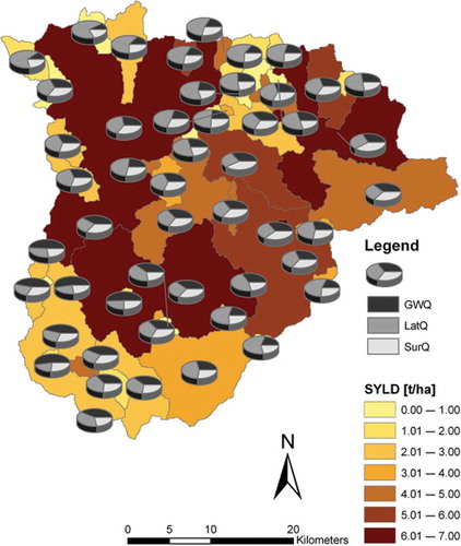
Our results show not only that the streamflow at the gauge is an important variable for analysing the water balance of a catchment, but also that the spatial patterns within the entire catchment are different. The combination of the main key factors, such as vegetation cover, slope and rainfall intensity, affects the spatial formation of surface runoff and, thus, the other flow components.

The relationship between surface runoff and erosion/sediment yield is well documented. So in a first step, the model set-up has been created to plausibly reflect the streamflow, the runoff components, but also their spatial patterns with sufficient accuracy. In a second step, this database is used for analysing erosion processes and sediment yield.

3.2 Sediment loads

3.2.1 Measured sediment data

During the field campaigns in October 2010 and February/March 2011, water samples were taken and suspended sediment was analysed at the 12 detailed sites (Table 11). The sediment concentrations were low (mean: 0.8 mg L^-1) depending on the low-flow conditions during the field campaigns. These values give an indication about the sediment concentrations during baseflow conditions. These measurement data were considered for model validation: simulated sediment concentrations during low-flow conditions resulted in a mean value of 1.2 mg L^-1 and fit within the range of measured values.

Table 11 Measured total suspended solids (TSS) at 12 detailed sites in two field campaigns in October 2010 and February/March 2011.

SWAT sub-basin	Date	TSS (mg L^-1)	Date	TSS (mg L^-1)
SUB05	19 October 2010	0.80	10 March 2011	0.22
SUB06	11 October 2010	0.40	11 March 2011	0.30
SUB19	26 October 2010	0.73	28 February 2011	0.51
SUB23	21 October 2010	0.95	1 March 2011	0.34
SUB07	9 October 2010	0.53	27 February 2011	0.51
SUB16	12 October 2010	5.40	26 February 2011	0.50
SUB17	16 October 2010	0.60	4 March 2011	0.41
SUB15	8 October 2010	0.55	9 March 2011	0.35
SUB18	10 October 2010	0.50	25 February 2011	0.73
SUB25	18 October 2010	1.67	14 March 2011	0.81
SUB43	17 October 2010	0.87	12 March 2011	0.34
SUB45	20 October 2010	0.20	13 March 2011	0.34
SUB18*	14 October 2010*	47.53
SUB25*	14 October 2010*	121.80

*Note: Two additional samples were taken after a heavy rain event.

Observations in the field show that after a heavy rain event the values increase strongly. Such an event happened on 14 October 2010, and the values increased to 47.53 (site SUB18) and 121.80 mg L^-1 (site SUB25), from values of 0.50 and 1.67 mg L^-1, respectively, four days before and after that event (see Table 11). This shows the high variability and fast response of sediment loads within the river depending on precipitation and streamflow. Even from this single rainfall event, conclusions about the monsoon period can be drawn: repeated rainfall results in very high sediment loads during monsoon periods.

Wang et al. (2013) conducted a suspended sediment monitoring in the Le’an river catchment (Fig. 2), which is part of the Raohe catchment of Poyang Lake basin. They took 17 water samples bi-monthly from June 2010 to July 2011 to analyse the suspended sediment concentration. As this catchment lies adjacent to our study area, both being sub-catchments of the Raohe, with similar climate, topography (13–1596 m a.s.l.), soils and fraction of forestland (71%), a comparison of the two study areas could be done. During the monitoring period, the suspended sediment concentrations ranged from 0.2 to 74.4 mg L^-1, with an average value of 9.99 mg L^-1. The mostly higher concentrations throughout the year can be explained by mining activities in the Le’an catchment.

Bieger (2013) also observed high variabilities of suspended sediment concentrations in a Chinese catchment (Xiangxi River, Hubei Province). Water samples taken during a flood event reached suspended sediment concentrations of up to 700 mg L^-1. Three days after the flood event, the values were orders of magnitude lower again.

3.2.2 Simulated sediment yields with SWAT

After analysing streamflow and water flow components, we analysed the temporal and spatial variability of the sediment yield (t ha^-1), i.e. the sediment from the sub-basin or HRU that is transported into the reach during the time step (Arnold et al. 2011).

3.2.2.1 Daily dynamics of sediment yield

Figure 6 shows the daily dynamics of the simulated sediment yield within the sub-basin at the basin outlet (site SUB45) over 10 years (2001–2010, calibration period). A correlation between high precipitation peaks and high sediment yield can be observed. The highest sediment peaks occur in the years 2002, 2003, 2006 and 2010 with (a) highest peaks and (b) highest annual sums. The maximum was in 2010, at 6.72 t ha^-1; the minimum sediment yield was in 2007, at 1.36 t ha^-1.

Fig. 6 Daily dynamics of the simulated sediment yield within the sub-basin at the basin outlet (SUB45) over 10 years (2001–2010, calibration period), as well as precipitation (CMA 2011). See Fig. 2 for catchment locations.

3.2.2.2 Monthly dynamics of sediment yield

Seasonal dynamics of the simulated sediment yield within the sub-basin at the basin outlet (SUB45) is shown as monthly sums averaged over 10 years (2001–2010, calibration period) in Fig. 7. It is shown that 69.8% of the simulated sediment yield occurs during the monsoon from March to July. This is in good agreement with the streamflow simulations: 71.6% discharge was calculated for the same period.

Fig. 7 Seasonal dynamics of the simulated sediment yield within the sub-basin at the basin outlet (site SUB45): values are the monthly sum of sediment yield averaged over 10 years (2001–2010, calibration period). See Fig. 2 for catchment locations.

In March, April, June and July, between 14.2 and 17.5% of annual sediment yield is simulated. There is one exception in May where only 5.4% of the annual sediment yield is modelled.

Downstream, beyond our study area, at Dufengkeng gauging station, 90.9% of sediment load occurs in the period March–July (1956–2005) (based on Ai 2007). Similar results are valid for Hushan gauging station in the Le’an catchment, both part of the Raohe catchment of the Poyang Lake basin. There, 92.58% of sediment load can be calculated for the months March–July (1956–2005, based on Sun 2010).

3.2.2.3 Spatial distribution of sediment yield between sub-basins

The sediment yield of all 50 sub-basins, represented as annual values averaged over 10 years (2001–2010) is shown in Fig. 5. The range is from 0 to 7 t ha^-1. There is no clear relationship: the lowest values are simulated at the outlet and adjacent sub-basins. Sub-basins near the basin borders do not show the highest values; these occur more frequently in the central part of the catchment. However, for the correlation between surface runoff and sediment yield for all 50 sub-basins, the coefficient of determination was calculated to 0.69.

The spatial variation of the sediment yield of the entire Yangtze basin, based on the sediment monitoring network, was examined by Yan et al. (2011). The range of values for the Poyang Lake sub-basin equals those from our modelling study (Table 6). Although slopes and landforms were considered, the authors emphasize that land use plays a major role in the sediment dynamics within the basins. The average soil erosion calculated by Lu et al. (2011) was higher for the entire Poyang Lake basin than in our sub-basin. They located the highly eroded areas mainly in the headstreams of the other four tributaries (Table 6). Also in the Liao watershed of the Poyang Lake area, soil erosion was much higher compared to our study area, possibly due to the smaller share of forest (59%; Li et al. 2010, Table 6).

Several studies were conducted in the Three Gorges area of Hubei Province (Fig. 2). Using the SWAT model, Bieger et al. (2013) simulated the sediment yield of the Xiangxi Catchment. Compared to our study area, simulated annual sediment yields were lower (Table 6). Also in that area, Shen et al. (2010) used the WEPP (Water Erosion Prediction Project) model to simulate the soil erosion distribution over the Zhangjiachong Watershed (1.62 km²). The main land uses are soil dike terraces, stone dike terraces, paddy fields, and mixed forest. The range of values is the same as in our modelling study, but Shen et al. (2010) did not calculate values up to 7 t ha^-1 as in our study.

The study of Lu et al. (2003) examined long-term sediment load data obtained in the Upper Yangtze basin. While the mean value is in the range of our modelling study, the highest sediment yield was not reached (Table 6), presumably due to the loess soil in the Upper Yangtze basin. A further SWAT study was conducted in the upper Yellow River watershed (Ouyang et al. 2010). The main soil erosion came from agricultural land, while relatively slight soil erosion was found in forests and on grassland in steep mountain areas. Soil erosion was much higher compared to our study area due to different climatic (continental cold and dry climate) and geologic conditions (dominated by Chestnut soils) (Table 6). Also Wu and Chen (2012) simulated a higher range of sediment yield at sub-basin level in a tributary of the Pearl River than in our modelling study (Fig. 2, Table 6). The authors relate the higher soil erosion rates to the high percentage of agricultural land (about 37%). In addition, they state that their results also indicate that erosion is quite sensitive to soil properties and slope.

3.2.2.4 Influence of land use on the spatial distribution of sediment yields

Considering our entire studied basin, the simulated total sediment load was 4.4 t ha^-1 (average annual basin value). However, the distribution of the loading in each sub-basin and HRU was different depending on slope, soil and land use. For the entire basin, the explicitly highest annual sediment loads were simulated for cabbage with 37.48 t ha^-1. Rice (2.23 t ha^-1) had higher loads than forest (0.18 t ha^-1) and tea (0.10 t ha^-1) (Table 12 left). Analysing HRUs with the same soil (ACu3 = Humic Acrisol) but different land uses within two example sub-basins, this relationship can be confirmed (Table 12 right). The small, more mountainous sub-basin SUB19 had slightly higher values as SUB45 at the basin outlet.

Table 12 Simulated sediment yield (SYLD; average annual values, 2001–2010) (left) for the entire basin depending on land use (LU) and (right) in HRUs of two example sub-basins with different land use and same soil (LU-Soil). n is the number of HRUs within the selected sub-basin.

LU	SYLD (t ha^-1)	SUB	LU-Soil	SYLD (t ha^-1)	n
Forest	0.18	19	FRST-ACu3	0.13	5
Tea	0.10		TEAT-ACu3	0.09	5
Cabbage	37.48		CABG-ACu3	32.66	4
Rice	2.23		RICE-ACu3	1.56	1
		45	FRST-ACu3	0.13	5
			TEAT-ACu3	0.08	4
			CABG-ACu3	26.11	4
			RICE-ACu3	1.27	1

Compared to the review of Hill and Peart (1998) about land use and erosion in southern China, the same range of values can be observed. They listed an average erosion rate of 0.05 t ha^-1 year^-1 for forest and woodland; the lowest rate for any given land-use cover. Cultivated slopes experience considerably higher erosion, with mean erosion rates of 62.4 t ha^-1 year^-1. Compared to the values of our modelling study, forest rates were higher (0.18 t ha^-1 year^-1) and for crop land with cabbage (37.5 t ha^-1 year^-1) lower. Hill and Peart (1998) stated that sediment yields from cultivated land are mostly about three orders of magnitude higher than from forest. In our study the ratio is around 1:200 between forest and cabbage cultivation.

El Kateb et al. (2013) observed at erosion plots in Shaanxi Province (Fig. 2) that soil loss was associated with rainfall intensity, vegetation covers and slope gradients; in fact, changes in soil loss were significantly higher than changes in the runoff. Our modelling study reveals 0.09% (SUB19) and 0.03% (SUB45) sediment yield of the total sediment yield (average values 2001–2010) of each sub-basin under forest cover, and 0.07% (SUB19) and 0.02% (SUB45) under tea cultivation. This is not directly comparable to the values from El Kateb et al. (2013; Table 7). But it shows that the differences of our simulated sediments results are much smaller between tea and forest (as already shown in Table 12). Furthermore, El Kateb et al. (2013) found out that soil losses in forests began at much higher runoff values than the other investigated land-use forms (Table 7).

Using the USLE, Zhang et al. (2011a) predicted the spatial distribution of the average annual soil loss in mountainous woodlands in China. The estimated national value (=0.0382 t ha^-1 year^-1) is lower than in our modelling study (0.18 t ha^-1 year^-1).

In the Shangshe catchment in the Anhui province (Fig. 2), field runoff observations were carried out and a new integral equation method used to calculate water and sediment discharge (Zhang et al. 2011b). Annual soil losses (2000–2007) from different land-use types (pine forest, Chinese fir forest, bamboo forest, and tea garden) were calculated. The values of Zhang et al. (2011b) are lower than in our modelling study (Table 7) but comparable as both study sites are located in Anhui province. The study also confirms soil erosion control due to intercepted rainfall, by weakening the kinetic energy of the raindrops, decreasing direct raindrop impact, improving soil structure for infiltration, absorbing surface runoff through litter and a well-developed root system. Furthermore, Zhang et al. (2011b) described a plot where the bush is changed to bare land, causing serious erosion with soil loss rates of up to 350 t ha^-1. When vegetation coverage increased to 70 and 80% through natural regeneration, the amount of soil erosion decreased significantly to around 3 t ha^-1. These values are relevant to our study because such processes are to be assumed in the areas that are clear-cut.

The RRC AP (Regional Resource Centre for Asia and the Pacific) (2001) report for Sri Lanka listed estimates of soil erosion in tea plantations from different literature sources. Considering tea during replanting, weeded tea, mulched and unmulched tea, well and poorly managed tea, the values range between 0.33 and 250 t ha^-1 year^-1. Our modelling study is close to the value of the well managed tea (Table 12). This should be evaluated critically because field observations showed that tea was planted both in a well and in a poorly managed way. Additionally, soil erosion depends on the growing stage of the tea trees and the use of hedgerows in the plots influencing soil stability (Shen et al. 2010, Table 7, Three Gorges Reservoir Area, Fig. 2).

The SWAT model results of Wu and Chen (2012) for the East River Basin showed higher sediment yields compared with our study for agricultural land and for the whole basin, but comparable values for forest (Table 7, Fig. 2).

Huang et al. (2010) conducted field experiments (2002–2007) in the red soil region in Hunan Province (Fig. 2) and compared soil erosion at conventional sloping farmland with three different reforestation types. Our modelling study revealed higher values for mixed forest, but also for sloping, conventional farmland with cabbage (Table 7).

The SWAT modelling study for the Xiangxi Catchment (Three Gorges Area, Fig. 2) determined 48 t ha^-1 of mean annual sediment yields from agricultural areas (Bieger et al. 2012). This is comparable to our SWAT model results for cropland (37.5 t ha^-1).

Long et al. (2006) analysed the relationship between land use and soil erosion in Zhongjiang, a typical agricultural county of Sichuan Province located in areas with severe soil erosion in the upper reaches of the Yangtze River (Fig. 2). Their results showed that the most serious soil erosion occurred on agricultural land with a slope of 10–25°. Both farmland and permanent crops were affected by soil erosion, with almost the same soil erosion for corresponding slope conditions.

A further study investigated the occurrence of soil erosion under coverage of Chinese cabbage. The experimental studies of Lee et al. (2010) in a Korean mountainous area resulted in lower soil loss compared to our model study (Table 7). One reason can be the occurrence of silty clay loam in their plot. Additionally they demonstrated the effect of reducing soil erosion by reduced tillage with or without rye mulching.

Chen et al. (2012) estimated the annual average soil erosion at rice fields on Taiwan (Fig. 2). The sediment yield of our modelling study is within the range of the different managed rice fields (Table 7).

3.2.2.5 Discussion on modelling of spatial sediment distribution

There are two sources of sediment in the SWAT model simulation: loadings from HRUs/sub-basins and channel degradation/deposition. While surface runoff is the primary factor controlling sediment loadings to the stream, there are a few other variables that affect sediment movement into the stream: tillage, the USLE equation support practices factor (USLE_P), the USLE equation cropping practices factor (USLE_C), the USLE equation slope length factor (SLSUBBSN) and the slope in the HRUs (Arnold et al. 2011). So, the performance of the model set-up is depending on several variables. The parameterization of the USLE factors was done as carefully as possible (Section 2.3) but it carries the risk of uncertainty due to the lack of measured sediment values for calibration and validation. A further uncertainty has to be assumed for the implementation of the land management as, on the one hand, data for the large catchment area had to be simplified; and on the other hand, knowledge on agricultural practices is not very detailed, despite interviews with farmers and literature review. An additional uncertainty occurs because no dams and reservoirs were implemented in the model set-up. This results in an uncertainty that affects mainly the retention of the catchment.

In the SWAT model, sediment yield is estimated for each HRU using the empirical MUSLE, which refers to sheet and rill erosion in fields. Sediment routing in the channel is affected either by sediment deposition or by channel degradation. Instream erosion analyses with higher spatial resolutions need the application of model cascades which also allow a further and more detailed consideration of different sediment pathways (Kiesel et al. 2013).

Simulated sediment generation is influenced by the parameterization of the MUSLE factors as well as of the spatial resolution of the SWAT calculation units. The plausibility of simulated sediment yields is limited by the non-linear relationship between sediment yield and HRU area in the MUSLE. FitzHugh and Mackay (2000) showed that sediment generation decreases substantially with decreases in sub-basin size. They account this trend primarily to the sensitivity of the runoff term in the MUSLE equation to HRU area, and also to changes in the statistical distribution of K and C factors throughout the watershed. Looking at HRU scale, Chen and Mackay (2004) calculated a decrease in sediment yield of 25% with a tenfold increase of HRU area, using unchanged USLE factors. They suggest a compensation of this aggregation effect by adjusting USLE factors. In our study, the parameterization of the MUSLE factors was done carefully. But for the steeply sloped areas there is still the potential risk of a representation of the spatial variation of surface runoff and sediment yields in the SWAT model. Bieger et al. (2015) analysed surface runoff and sediment yields at the HRU level in the Chinese Xiangxi catchment. The simulated spatial variability of surface runoff and sediment yields with slope was not consistently plausible. They discovered that neither surface runoff nor sediment yields showed a plausible increase with increasing slope gradients. For surface runoff, they explain this with minor simplifications in some SWAT algorithms that only affect steeply sloping watersheds, e.g. concerning the curve number, and with the strong indirect impact of lateral flow on surface runoff.

In addition, further research questions show the need and importance of spatial sediment data. Results from hydrological models have been used to study aquatic ecosystems in ecohydrological studies (Schmalz et al. 2012). Previous studies in the study catchment with a preliminary ecohydrological model resulted in the successful transference of data to a species distribution model (Kuemmerlen et al. 2012). As the flow regime and sediment loads and their dynamics play a significant role in shaping the biotic community in streams, the availability of modelled data allows them to be included in ecological models where a high temporal and spatial resolution is required (Allan et al. 1997, Jähnig et al. 2012, Kuemmerlen et al. 2014).

4 CONCLUSION AND OUTLOOK

The study analyses assessment of the spatial distribution of surface runoff and sediment yield in a data-scarce Chinese river basin. As in many other areas in China, streamflow, but not sediment data, is measured continuously. In addition, there are no studies about soil erosion and sediment entry into the rivers.

Our study presents an approach for dealing with such data scarcity in order to derive the spatial distribution of surface runoff and sediment yield. The method developed herein used field observations, measured data and literature research to fix in advance as many parameters as possible during parameterization of water flow and sediment variables of the process-based, ecohydrological model SWAT. For this study, it was more important to represent the field observations and the processes in the catchment than perform an auto-calibration with a possibly better model performance. A semi-calibration was conducted: only streamflow was calibrated and validated with long-term measured data, whereas the modelled sediment yield data were checked separately. After calculating streamflow and suspended sediment at the basin outlet as well as surface runoff and sediment yield for the sub-basins with SWAT, we validated and checked the credibility of our simulated results using published literature on land use and associated land management. Several studies were already conducted in China analysing erosion processes and sediment yield. Some of these used experimental fields or plot studies, others catchment-scale and modelling studies. They were compared to our model results for validation purposes. Because there are no measured long-term sediment data, we needed this validation of our model results derived from other studies. We used their investigated relationships between land use and sediment yield and transferred the findings and parameter ranges onto our results.

Our analyses, as well as those of previous studies, show that vegetation cover and land management are key factors affecting surface runoff and erosion. Our modelling results show that the highest amounts of surface runoff and sediment yield occur on agricultural land, particularly on cropland with cabbage cultivation. In contrast, forest shows only very slight erosion. Additionally, flow components and sediment yield are related to topographical characteristics such as mountainous or flat areas. Besides a temporal variability due to the monsoon climate, the spatial variability caused by different land use, slope and soil results in different flow component and erosion patterns between the studied sub-basins.

The advantage of this approach is that, once the model is set up: (a) the parameterization can be changed easily with a shorter calibration procedure than usual, if new field or literature data are available and need to be be fixed; and (b) the validation can be extended to further factors, such as slopes or soils. Transferring the presented parameterization to other catchments is only useful if the basin conditions, especially slope, soil and land-use conditions, are the same. However, the entire approach can be applied in any data-scarce region and shows a procedure for dealing with regions in which continuous data are missing. Landscape planning or water management need an area-wide database which is provided by this procedure.

Further steps are needed to improve this approach and to transfer it to other study areas. Future studies should implement a comprehensive analysis on further key factors such as soils, slopes and climate distribution, because our study concentrated on the relationship and impact of land use and agricultural management on the spatial distribution of sediment yields.

In addition, this approach can help to identify areas with high erosion potential and can be used to plan erosion control measures. If the current state is known, model scenarios can follow up to evaluate proposed measures and reduce sediment discharge in the future. The possible impact of land-use and climate change, and the resilience of the catchment as a unit can also be analysed using this model set-up.

Disclosure statement

No potential conflict of interest was reported by the author(s).

Acknowledgements

Our thanks go to Prof. Dr Jiang Tong, China Meteorological Administration, Beijing, for his friendly support. Additionally, we like to thank Song Song, Alexander Strehmel, Yang Shun Yi, Wang Xing Zhong, Sun Xiaoling and Dong Xiaoyu for their help during the field campaigns and/or lab analyses.

Additional information

Funding

The DFG (German Research Foundation) project “Integrated modelling of the response of aquatic ecosystems to land use and climate change in the Poyang Lake region, China” is part of the NSFC/DFG joint funding programme “Land Use and Water Resources Management under Changing Environmental Conditions”. We thank the DFG for financial support (F0 301/14-1, JA 1827/2-1).

REFERENCES

- Abbaspour, K.C., 2007. User manual for SWAT-CUP, SWAT calibration and uncertainty analysis programs. Eawag, Duebendorf: Swiss Federal Institute of Aquatic Science and Technology.
- AELF, 2011. Information about china cabbage [online]. Deggendorf: Amt für Ernährung, Landwirtschaft und Forsten Deggendorf. Available from: http://www.aelf-dg.bayern.de/index.php [Accessed 29 July 2011].
- Ai, Q., 2007. Analysis on the changes of sediment of Changjiang basin. JiangXi Energy, 1, 28–30.
- Allan, D., Erickson, D., and Fay, J., 1997. The influence of catchment land use on stream integrity across multiple spatial scales. Freshwater Biology, 37 (1), 149–161. doi:10.1046/j.1365-2427.1997.d01-546.x
- Anhui Statistical Bureau, 2010. Anhui statistical yearbook 2010. Beijing: China Statistics Press. English and Chinese.
- Arnold, J.G. and Allen, P.M., 1999. Automated methods for estimating baseflow and groundwater recharge from streamflow records. Journal of the American Water Resources Association, 35 (2), 411–424. doi:10.1111/j.1752-1688.1999.tb03599.x
- Arnold, J.G., et al., 1995. Automated base flow separation and recession analysis techniques. Ground Water, 33 (6), 1010–1018. doi:10.1111/j.1745-6584.1995.tb00046.x
- Arnold, J.G., et al., 1998. Large area hydrologic modeling and assessment Part I: model development. Journal of the American Water Resources Association, 34 (1), 73–89. doi:10.1111/j.1752-1688.1998.tb05961.x
- Arnold, J.G., et al., 2011. Soil and Water Assessment Tool – Input/Output File Documentation – Version 2009. Grassland, TX, Soil and Water Research Laboratory – Agricultural Research Service. Blackland Research Center – Texas AgriLife Research. Texas Water Resources Institute TR-365.
- Berry, L., 2003. Land degradation in China: its extent and impact. In: L. Berry, J. Olson, and D. Campbell, eds. Assessing the extent, cost and impact of land degradation at the national level. Findings and lessons learned from seven pilot case studies[online]. Commissioned by Global Mechanism with support from the World Bank. Available from: http://www.researchgate.net/publication/272682048_Assessing_The_Extent_Cost_And_Impact_Of_Land_Degradation_At_The_National_Level_Findings_And_Lessons_Learned_From_Seven_Pilot_Case_Studies [Accessed 24 February 2015].
- Bieger, K., 2013. Assessing the impact of land use change on hydrology and sediment yield in the Xiangxi Catchment (China) using SWAT [online]. Dissertation, Christian-Albrechts-Universität zu Kiel. Available from: http://eldiss.uni-kiel.de/macau/receive/dissertation_diss_00011201 [Accessed 15 July 2013].
- Bieger, K., Hörmann, G., and Fohrer, N., 2012. Simulation of streamflow and sediment with the soil and water assessment tool in a data scarce catchment in the Three Gorges Region, China. Journal of Environmental Quality. doi:10.2134/jeq2011.0383.
- Bieger, K., Hörmann, G., and Fohrer, N., 2013. The impact of land use change in the Xiangxi Catchment (China) on water balance and sediment transport. Regional Environmental Change, 15 (3), 485–498. doi:10.1007/s10113-013-0429-3.
- Bieger, K., Hörmann, G., and Fohrer, N., 2015. Detailed spatial analysis of SWAT-simulated surface runoff and sediment yield in a mountainous watershed in China. Hydrological Sciences Journal. doi:10.1080/02626667.2014.965172.
- Chen, E. and Mackay, D.S., 2004. Effects of distribution-based parameter aggregation on a spatially distributed agricultural nonpoint source pollution model. Journal of Hydrology, 295, 211–224. doi:10.1016/j.jhydrol.2004.03.029
- Chen, J., 2007. Rapid urbanization in China: a real challenge to soil protection and food security. Catena, 69, 1–15. doi:10.1016/j.catena.2006.04.019
- Chen, S.-K., Liu, C.-W., and Chen, Y.-R., 2012. Assessing soil erosion in a terraced paddy field using experimental measurements and universal soil loss equation. Catena, 95, 131–141. doi:10.1016/j.catena.2012.02.013
- Chen, Z., et al., 2001. Yangtze River of China: historical analysis of discharge variability and sediment flux. Geomorphology, 41, 77–91. doi:10.1016/S0169-555X(01)00106-4
- Chow, V.-T., 1959. Open channel hydraulics. New York: McGraw-Hill.
- CMA (Chinese Meteorological Administration), 2011. Daily climate data 1960–2010 from the stations Jingdezhen (58527), Meilin/Tunxi (58531) and Anqing (58424).
- Domrös, M. and Gongbing, P., 1988. The climate of China. Berlin: Springer.
- El Kateb, H., et al., 2013. Soil erosion and surface runoff on different vegetation covers and slope gradients: a field experiment in southern Shaanxi Province, China. Catena, 105, 1–10. doi:10.1016/j.catena.2012.12.012
- FAO, 2006. World reference base for soil resources. Rome: FAO. World Soil Resources Reports no. 103. ISBN 92-5-105511-4.
- FAO/IIASA/ISRIC/ISSCAS/JRC, 2009. Harmonized world soil database (version 1.1). Rome: FAO.
- FitzHugh, T.W. and Mackay, D.S., 2000. Impacts of input parameter spatial aggregation on an agricultural nonpoint source pollution model. Journal of Hydrology, 236, 35–53. doi:10.1016/S0022-1694(00)00276-6
- Gupta, H.V., Sorooshian, S., and Yapo, P.O., 1999. Status of automatic calibration for hydrologic models: comparison with multilevel expert calibration. Journal of Hydrologic Engineering, 4 (2), 135–143. doi:10.1061/(ASCE)1084-0699(1999)4:2(135)
- Hao, F.-H., Chang, Y., and Ning, D.-T., 2004. Assessment of China’s economic loss resulting from the degradation of agricultural land in the end of 20th century. Journal of Environmental Sciences, 16 (2), 199–203.
- Hill, R.D. and Peart, M.R., 1998. Land use, runoff, erosion and their control: a review for southern China. Hydrological Processes, 12, 2029–2042.
- Huang, Z., et al., 2010. Response of runoff and soil loss to reforestation and rainfall type in red soil region of southern China. Journal of Environmental Sciences, 22 (11), 1765–1773. doi:10.1016/S1001-0742(09)60317-X
- ISRIC, 2010. ISRIC data base China: world soil information [online]. Available from: http://www.isric.org/data/soil-and-terrain-database-china [Accessed 13 March 2015].
- Jähnig, S.C., et al., 2012. Modelling of riverine ecosystems by integrating models: conceptual approach, a case study and research agenda. Journal of Biogeography, 39, 2253–2263. doi:10.1111/jbi.12009
- Jarvis, A., et al., 2008. Hole-filled seamless SRTM data V4 [online]. International Centre for Tropical Agriculture (CIAT). Available from: http://srtm.csi.cgiar.org [Accessed 7 July 2010].
- Jiangxi Hydrological Bureau, 2011. Tankou gauging station (province Jiangxi): daily discharge data 1981–2010.
- Jingdezhen Environmental Protection Bureau, 2011. Climate information about Poyang lake area [online]. Available from: www.jdz65.gov.cn [Accessed 12 July 2011].
- Kiesel, J., et al., 2013. Application of a hydrological-hydraulic modelling cascade in lowlands for investigating water and sediment fluxes in catchment, channel and reach. Journal of Hydrology and Hydromechanics, 61 (4), 334–346. doi:10.2478/johh-2013-0042
- Kuemmerlen, M., et al., 2012. Integrierte Modellierung von aquatischen Ökosystemen in China: Arealbestimmung von Makrozoobenthos auf Einzugsgebietsebene. Hydrologie und Wasserbewirtschaftung, 56 (4), 185–192.
- Kuemmerlen, M., et al., 2014. Integrating catchment properties in small scale species distribution models of stream macroinvertebrates. Ecological Modelling, 277, 77–86. doi:10.1016/j.ecolmodel.2014.01.020
- Lal, R., 2007. Anthropogenic influences on world soils and implications to global food security. Advances in Agronomy, 93, 69–93. doi:10.1016/S0065-2113(06)93002-8
- Lattauschke, G., 2006. Chinakohl. Sächsische Landesanstalt für Landwirtschaft Gartenakademie [online]. Available from: http://www.umwelt.sachsen.de/lfl/publikationen/download/2248_1.pdf. [Accessed 29 July 2011].
- Lee, J.T., et al., 2010. Application of reduce tillage with a strip tiller and its effect on soil erosion reduction in highland agriculture. In: 19th world congress of soil science, soil solutions for a changing world, 1–6 August, Brisbane. Available from: http://www.iuss.org/19th%20WCSS/Symposium/pdf/1119.pdf.
- Li, H., et al., 2010. Assessment of soil erosion and sediment yield in Liao watershed, Jiangxi Province, China, Using USLE, GIS, and RS. Journal of Earth Science, 21 (6), 941–953. doi:10.1007/s12583-010-0147-4
- Li, X.-H., Zhang, Q., and Xu, C.-Y., 2012. Suitability of the TRMM satellite rainfalls in driving a distributed hydrological model for water balance computations in Xinjiang catchment, Poyang lake basin. Journal of Hydrology, 426-427, 28–38. doi:10.1016/j.jhydrol.2012.01.013
- Liang, X.Q., et al., 2013. Mitigation of nutrient losses via surface runoff from rice cropping systems with alternate wetting and drying irrigation and site-specific nutrient management practices. Environmental Science and Pollution Research. doi:10.1007/s11356-012-1391-1
- Long, H.L., et al., 2006. Land use and soil erosion in the upper reaches of the Yangtze River: some socio-economic considerations on China’s Grain-For-Green Programme. Land Degradation & Development, 17, 589–603. doi:10.1002/ldr.736
- Lu, J., et al., 2011. Soil erosion changes based on GIS/RS and USLE in Poyang Lake basin. Transactions of the CSAE, 27 (2), 337–345 (in Chinese).
- Lu, J., Liu, Y., and Chen, Y., 2004. Soil fertility degradation in eroded hilly red soils of China. In: M.J. Wilson, Z. He, and X. Yang, eds., The red soils of China: their nature, management and utilization. Dordrecht: Kluwer.
- Lu, X.X., Ashmore, P., and Wang, J., 2003. Sediment yield mapping in a large river basin: the Upper Yangtze, China. Environmental Modelling and Software, 18, 339–353. doi:10.1016/S1364-8152(02)00107-X
- Moriasi, D.N., et al., 2007. Model evaluation guidelines for systematic quantification of accuracy in watershed simulations. Transactions of the ASABE, 50, 885–900. doi:10.13031/2013.23153
- Nash, J.E. and Sutcliffe, J.V., 1970. River flow forecasting through conceptual models, Part I—A discussion of principles. Journal of Hydrology, 10, 282–290. doi:10.1016/0022-1694(70)90255-6
- Neitsch, S.L., et al., 2010. Soil and Water Assessment Tool – Input/Output File Documentation – Version 2009. Grassland, TX, Soil and Water Research Laboratory, Agricultural Research Service. Blackland Research Center, Texas AgriLife Research. Texas Water Resources Institute TR-365.
- Neitsch, S.L., et al., 2011. Soil and Water Assessment Tool – Theoretical Documentation – Version 2009. Grassland, TX, Soil and Water Research Laboratory, Agricultural Research Service. Blackland Research Center, Texas AgriLife Research. Texas Water Resources Institute TR-406.
- Ouyang, W., et al., 2010. Soil erosion dynamics response to landscape pattern. Science of the Total Environment, 408, 1358–1366. doi:10.1016/j.scitotenv.2009.10.062
- Overton, D.E., 1966. Muskingum flood routing of upland streamflow. Journal of Hydrology, 4, 185–200. doi:10.1016/0022-1694(66)90079-5
- Pan, X. and Shi, Q., 2002. Low yields of double-crop rice in Jiangxi Province—causes and countermeasures study. Rice Circle, 4, 2 p. (in Chinese).
- RRC AP (Regional Resource Centre for Asia and the Pacific), 2001. State of the Environment Report Sri Lanka 2001. Part III Priority Issues [online]. Available from: http://www.rrcap.ait.asia/pub/soe/srilanka_land.pdf [Accessed 2 August 2013]
- Ruan, J., Guan, Y.L., and Wu, X., 2002. Status of Mg availability and the effects of Mg application in tea fields of Red Soil area in China. Scientia Agricultura Sinica, 35 (7), 815–820. (In Chinese with English abstract).
- Schmalz, B., et al., 2012. Integrierte Modellierung von aquatischen Ökosystemen in China: Ökohydrologie und Hydraulik. Hydrologie und Wasserbewirtschaftung, 56 (4), 169–184.
- Schönbrodt, S., et al., 2010. Assessing the USLE crop and management factor C for soil erosion modeling in a large mountainous watershed in Central China. Journal of Earth Science, 21 (6), 835–845. doi:10.1007/s12583-010-0135-8
- Shen, Z., et al., 2010. Analysis and modeling of soil conservation measures in the Three Gorges Reservoir Area in China. Catena, 81, 104–112. doi:10.1016/j.catena.2010.01.009
- Song, S., 2011. Interviews with Chinese farmers in the Poyang area in February and March 2011. Personal communication.
- Sun, P., 2010. Spatio-temporal patterns of sediment and runoff changes in the Poyang lake basin and underlying causes. Acta Geographica Sinica, 7, 828–839.
- Wang, Z., et al., 2013. The spatiotemporal variations of suspended sediment concentration in Le’an river catchment of Poyang lake basin. Advanced Materials Research, 610-613, 1099–1102. doi:10.4028/www.scientific.net/AMR.610-613.1099., Trans Tech Publications, Switzerland.
- Williams, J.R., 1969. Flood routing with variable travel time or variable storage coefficients. Transactions of the ASAE, 12 (1), 100–103. doi:10.13031/2013.38772
- Williams, J.R., 1975. Sediment routing for agricultural watersheds. Journal of the American Water Resources Association, 11, 965–974. doi:10.1111/j.1752-1688.1975.tb01817.x
- Wu, X.-Y., et al., 2011. Nitrogen loss in surface runoff from Chinese cabbage fields. Physics and Chemistry of the Earth, Parts A/B/C, 36, 401–406. doi:10.1016/j.pce.2010.11.004
- Wu, Y. and Chen, J., 2012. Modeling of soil erosion and sediment transport in the East River Basin in southern China. Science of the Total Environment, 441, 159–168. doi:10.1016/j.scitotenv.2012.09.057
- Yan, Y., Wang, S., and Chen, J., 2011. Spatial patterns of scale effect on specific sediment yield in the Yangtze River basin. Geomorphology, 130, 29–39. doi:10.1016/j.geomorph.2011.02.024
- Yang, A., et al., 2002. Soil erosion characteristics and control measures in China. In: J. Jiao ed. 12th ISCO Conference Beijing 2002, 26–31 May, Beijing, 463–469. Available from: http://tucson.ars.ag.gov/isco/isco12/info.html
- Yang, G., et al., 2007. Sediment rating parameters and their implications: Yangtze River, China. Geomorphology, 85, 166–175. doi:10.1016/j.geomorph.2006.03.016
- Ye, L. and Van Ranst, E., 2009. Production scenarios and the effect of soil degradation on long-term food security in China. Global Environmental Change, 19, 464–481. doi:10.1016/j.gloenvcha.2009.06.002
- Ye, X., Zhang, Q., and Viney, N.R., 2011. The effect of soil data resolution on hydrological processes modelling in a large humid watershed. Hydrological Processes, 25, 130–140. doi:10.1002/hyp.7823
- Yule, G.U., 1899. An investigation into the causes of changes in Pauperism in England, Chiefly during the last two intercensal decades (Part I.). Journal of the Royal Statistical Society, 62, 249–295. doi:10.2307/2979889
- Zhang, J. and Lin, Z., 1992. Climate of China. New York: John Wiley and Sons, 376 p.
- Zhang, Q., et al., 2006. Sediment and runoff changes in the Yangtze River basin during past 50 years. Journal of Hydrology, 331, 511–523. doi:10.1016/j.jhydrol.2006.05.036
- Zhang, C., et al., 2011a. Assessment of soil erosion under woodlands using USLE in China. Frontiers of Earth Science, 5 (2), 150–161. doi:10.1007/s11707-011-0158-1
- Zhang, J.C., De Angelis, D.L., and Zhuang, J.Y., eds., 2011b. Calculation of water and sediment discharge using an integral calculus method. In: Theory and practice of soil loss control in eastern China. New York: Springer, 31–46.