The influence of parametric uncertainty on the relationships between HBV model parameters and climatic characteristics

Abstract

An HBV rainfall–runoff model was applied to test the influence of climatic characteristics on model parameter values. The methodology consisted of the calibration and cross-validation of the HBV model on a series of 5-year periods for four selected catchments (Axe, Kamp, Wieprz and Wimmera). The model parameters were optimized using the SCEM-UA method which allowed for their uncertainty also to be assessed. Nine climatic indices were selected for the analysis of their influence on model parameters, and divided into water-related and temperature-related indices. This allowed the dependence of HBV model parameters on climate characteristics to be explored following their response to climate change conditioned on the catchment’s physical characteristics. The Pearson correlation coefficient and weighted Pearson correlation coefficient were used to test the dependence. Most parameters showed a statistically significant dependence on several climatic indices in all catchments. The study shows that the results of the correlation analysis with and without parametric uncertainty taken into account differ significantly.

Résumé

Le modèle pluie-débit HBV a été appliqué pour tester l’influence des conditions climatiques sur les valeurs des paramètres du modèle. La méthodologie consiste à caler et valider le modèle HBV sur des périodes de cinq ans pour quatre bassins (Axe, Kamp, Wieprz and Wimmera). Les paramètres du modèle ont été optimisés grâce à la méthode SCEM-UA qui permet d’estimer l’incertitude. Neuf indices climatiques ont été sélectionnés pour analyser leur influence sur les paramètres du modèle, et on été répartis entre indices liés à l’eau et indices liés à la température. Cela a permis d’explorer la dépendance des paramètres de HBV aux caractéristiques climatiques en observant leur réponse au changement climatique selon les caractéristiques physiques du bassin. Le coefficient de corrélation de Pearson et le coefficient de corrélation de Pearson pondéré ont été utilisés pour tester la dépendance des paramètres du modèle aux indices climatiques. La plupart des paramètres a montré une dépendance statistiquement significative à plusieurs indices climatiques pour tous les bassins. L’étude montre que les résultats de l’analyse de la corrélation avec et sans prise en compte de l’incertitude paramétrique diffère significativement.

Key words:

• hydrological modelling
• HBV
• calibration
• validation
• non-stationarity of model parameters
• climate change

Mots clefs:

• HBV
• calage
• validation
• non-stationnarité des paramètres des modèles
• changement climatique

1 INTRODUCTION

Climate projections published by the Intergovernmental Panel on Climate Change in their Fifth Assessment Report (IPCC 2013) indicate an increase in the variability of precipitation, which will in turn lead to larger seasonal variations in runoff in many areas. According to the information provided (Christensen et al. 2013) the effect of climate change on hydrological process will be spatially varied, leading to more frequent occurrence of extreme hydrological conditions (floods and droughts). Projected increases in temperature will also have consequences for hydrological regimes, such as a reduction in winter snow storage, a larger volume of winter precipitation falling as rainfall, and increases in potential evapotranspiration. All these expected changes indicate possible changes in catchment processes, and in particular, the hydrological cycle. The hydrological impacts of climate change may be assessed using hydrological models calibrated on available historical data and run using predicted future climatic forcing. This approach assumes that catchment processes are stationary. Many scientists have realized that this assumption contradicts the main goal of the research undertaken, i.e. the prediction of changes in hydrological regimes in a changing climate (e.g. Li et al. 2012). In addition, rainfall–runoff models applied for the estimation of future hydrological changes are usually calibrated using particular performance criteria, such as the Nash-Sutcliffe coefficient (Nash and Sutcliffe 1970). That type of criterion favours model parameters that give good model performance for average to high flow values (Gupta et al. 2009), but might not be suitable for simulating future low and high extreme flow events. A discussion of different aspects of model calibration and model reliability is given by Seibert (2003), who used a differential split-sample test on four different catchments and included additional groundwater level data for calibration. His results showed that model simulations obtained outside the parameter calibration range should be treated with caution. The transferability of hydrological model parameters under varying climatic conditions was investigated by Vaze et al. (2010) and Li et al. (2012) for Australian catchments. Both studies found that model parameters depend on climatic characteristics and that their temporal transferability depends on both climatic and physical catchment conditions. The division of time periods into dry and wet weather conditions allowed for the illustration of the dependence of model parameters on climate.

Singh et al. (2011) studied 294 USA catchments. They conditioned (calibrated) catchment model parameters on climatic characteristics, such as runoff ratio (the long-term ratio of streamflow to precipitation) and baseflow index (the long-term ratio of baseflow to total streamflow). The results indicated that the catchment response to climate variability is stronger when taking into account the dependence of model parameters on climatic characteristics, especially for high and low flow conditions.

Previously, the generally advised length of the calibration period exceeded several years to capture the variability of climatic conditions (e.g. Sorooshian and Gupta 1983). That approach assumed that climatic processes are stationary and therefore the model parameters are constant. However, when a change of parameters is expected due to a changing climate, the calibration time horizon should be shorter. Merz et al. (2011) analysed the change of parameters of rainfall–runoff models calibrated to six consecutive 5-year periods between 1976 and 2006 for 273 catchments in Austria. The results of that study indicated statistically-significant temporal trends for HBV parameters related to snow and soil moisture. The tendency and slope were similar for different regions of Austria indicating a rather general tendency. The trends found in parameter values were attributed to changes in climatic conditions. The analysis indicated a large variability in the correlation between model parameters and climatic indices for the analysed catchments, which may be attributed to differences in the hydrological processes in catchments and parameter identifiability problems.

The present paper extends the work of Merz et al. (2011) in two ways: by the extension of the study area to catchments located in various climatic zones and taking into account model parameter uncertainty. The parametric uncertainty is taken into account by using the Weighted Pearson Correlation Coefficient (WPCC) to analyse the relationships between the HBV model parameters estimated by the SCEM-UA optimization method, developed by Vrugt et al. (2003), and climatic indices.

The research done so far shows that the problem is complex and depends both on climatic and catchment characteristics. The novelty of the present research lies in looking at the problem of parameter nonstationarity from a different perspective, i.e. looking at the physical interpretation of possible changes. Specifically, the goal of the paper is to investigate the dependence of the parameters of the conceptual model HBV (Bergström 1995) on climate indices, for a number of catchments varying in size and water availability, taking into account the physical interpretation of the parameters. This paper is part of a larger project aiming at the analysis of the nonstationarity of hydrological model parameters under varying conditions (Thirel et al. 2015). In the framework of this project, a common hydro-meteorological database with data from 14 catchments was provided. The project participants tested the application of hydrological models under changing conditions at various temporal scales. We focus on the influence of varying climatic conditions whilst assuming a stable land use. The paper’s goal was carried out by: (a) calibration of a conceptual rainfall–runoff model (HBV) using a 5-year moving window and cross-validation of the model parameters; (b) analysis of the temporal variability of the HBV model parameters and climatic indices; and (c) analysis of the dependence of model parameters on climatic indices taking into account parametric uncertainty.

Section 2 presents the study catchments and describes the physical characteristics of the catchments. Section 3 presents the methodology including the choice of climatic indices, a description of the hydrologic model HBV, simplification of the model structure using the sensitivity analysis, methods used for the model calibration and validation, and the methods applied to study the correlation between parameters and climatic indices. Section 4 describes the results of the study including the temporal variability of climatic indices, a summary of the calibration and validation results and temporal variability of HBV model parameters, followed by a discussion of the dependence of model parameters on climatic indices. Conclusions are presented in Section 5.

2 STUDY CATCHMENTS

In this paper we analysed three catchments selected from the database provided in the framework of the IAHS Workshop Testing simulation and forecasting models in nonstationary conditions (held in Göteborg, Sweden, July 2013), and an additional catchment, Wieprz, located in Poland. A detailed description of the catchments from the workshop database is provided by Thirel et al. (2015). The chosen catchments are characterized by stable land-use conditions, the availability of input data (precipitation, air temperature, potential evapotranspiration) and their suitability for the HBV modelling.

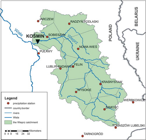
The Wieprz catchment is located in eastern Poland, the River Wieprz being a tributary of the River Vistula. The catchment area (approx. 10 231 km²) is located entirely within the administrative boundaries of Lublin province. The catchment elevation ranges from the 115 m a.s.l. at the gauging station to about 390 m a.s.l. for the highest hills. According to the Corine Landcover data for the year 2000, it is covered by agricultural areas (77%), forest and semi-natural areas (19%), artificial surface (3%) and water bodies (1%). Comparison of Corine Landcover data from the years 1990, 2000 and 2006 indicates relatively stable land-use conditions in this catchment.

In this study we use flow observations from the Kośmin gauging station. The rainfall and temperature data are based on observations from the Puławy, Sobieszyn, Lublin, Tarnogród, Zamość, and Tomaszów Lubelski meteorological stations. Figure 1 shows a map of the Wieprz catchment together with the location of the hydro-meteorological stations.

Fig. 1 Map of the Wieprz catchment together with the location of hydro-meteorological stations.

As is evident from Table 1, the catchments differ in size and geographic location, implying that the climatic conditions are also different.

Table 1 The catchments selected for study.

Catchment	Country	Catchment area (km^2)	References
Axe Creek at Longlea	Australia	237	Potter and Chiew (2011) Vaze et al. (2011)
River Kamp at Zwettl	Austria	622	Blöschl et al. (2008) Komma et al. (2007) Reszler et al. (2008)
River Wieprz at Kosmin	Poland	10 231	Romanowicz et al. (2013)
River Wimmera at Glenorchy Weir Tail	Australia	2000	Potter and Chiew (2011) Vaze et al. (2011)

3 METHODOLOGY

3.1 Climatic indices

There are many different indices that can be used to describe the variability of climatic conditions influencing hydrological model parameters (e.g. Van Werkhoven et al. 2008, Merz et al. 2011). The most relevant variables for the modelling of hydrological processes are precipitation, air temperature and potential evapotranspiration (PET). From a systems theory point of view, the model should be stimulated by strong and highly variable input for the model parameters to be identified (e.g. Schweppe 1973). For this reason, we analyse the mean of climatic characteristics over the time window (five years) and the variability of climatic characteristics measured by their standard deviation. For each time window of 5 years we determined the following climatic indices:

• mean P: mean precipitation;

• std P: standard deviation of daily precipitation;

• NW: number of wet days estimated from catchment average precipitation;

• mean PW: mean wet day precipitation;

• std PW: standard deviation of wet day precipitation;

• mean PET: mean daily PET;

• std PET: standard deviation of daily PET;

• mean T: mean daily air temperature; and

• std T: standard deviation of daily air temperature.

Altogether we have nine indices that describe climatic conditions and examine herein their variability within the chosen observation period. As some of these indices are correlated with each other, their joint impact on the model performance should be assessed with care. Further, we study the degree of correlation between climatic indices and HBV parameters using statistical methods (the Pearson correlation coefficient and its weighted version). The nine chosen indices can be roughly divided into two groups: precipitation-related and temperature-related. The first group includes mean P, std P, NW, mean PW and std PW. The number of wet days (days with precipitation >0.1 mm/d) was calculated based on the catchment average precipitation. These values depend on the catchment size and the number of precipitation stations. The second group includes indices based on direct observations of temperature (mean T, std T), and those derived from temperature, based on PET (mean PET, std PET). As mentioned, the indices within groups may be correlated. In particular, there is a strong correlation between indices related directly to temperature and those that are temperature-derived, i.e. PET. Nevertheless, each of the indices carries different information on climatic conditions and its relationship to the HBV model parameters might be different.

3.2 Hydrological model

The rainfall–runoff model applied in this paper is the lumped conceptual HBV model (Bergström 1995, Lindström 1997, Lindström et al. 1997, Booij 2005, Booij and Krol 2010). It has often been used to study the influence of climate change on water resources (Bergström et al. 2001, Andréasson et al. 2004, Graham et al. 2007, Akhtar et al. 2008, Olsson and Lindström 2008, Van Pelt et al. 2009, Arheimer et al. 2011, Cloke et al. 2013, Demirel et al. 2013). The model has a physically-based structure that includes four conceptual storage reservoirs describing snowmelt, soil moisture, and runoff components of the rainfall–runoff processes in the catchment (Fig. 2). In this study the model was run on a daily basis. Due to the different sources of data, PET was calculated using different methods:

• Axe and Wimmera catchments—Morton’s wet environment evapotranspiration algorithm (Potter and Chiew 2011);

• Kamp catchment—modified Blaney-Criddle method (Parajka et al. 2007); and

• Wieprz catchment—Hamon method based on air temperature (Hamon 1961).

Fig. 2 Structure of the HBV model applied in this study.

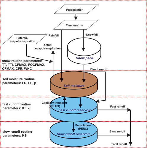
The lumped HBV model is a simplified representation of spatially varying rainfall–runoff processes in a catchment. Therefore, model parameters have only a very crude resemblance to their physical counterparts. The structure of the HBV model used is presented in Fig. 2. The model has fourteen parameters. These are FC: maximum soil moisture storage (mm), β: nonlinear runoff parameter, LP: limit for potential evapotranspiration, α: nonlinear response parameter, KF: upper storage coefficient (1/d), KS: lower storage coefficient (1/d), PERC: percolation rate (mm/d), CFLUX: maximum capillary rate (mm/d), TT: threshold temperature (°C), TTI: temperature threshold interval length (°C), CFMAX: degree-day factor (mm/°Cd), FOCFMAX: CFMAX (degree-day factor) corrected for forests (mm/°Cd), CFR: refreezing factor of water released from melting snow (-), and WHC: water holding capacity of snow (mm/mm).

The precipitation, PET and temperature are external driving forces. Parameters TT, TTI, CFMAX, FOCFMAX, CFR and WHC are related to snow processes. The FC, LP and β parameters are related to the soil moisture processes in the catchment (unsaturated zone). CFLUX represents the capillary transport between the fast runoff reservoir and the soil moisture reservoir. The fast runoff is described by the KF and α parameters. PERC describes the transport between the fast and slow runoff reservoirs (percolation). The slow runoff reservoir is represented by the KS parameter.

3.3 Model simplification

The selected version of the HBV model includes 14 parameters and could suffer from equifinality problems (Beven 2006). To simplify the model, a sensitivity analysis using the Morris method was applied (Morris 1991). In this method the sensitivity is estimated on the basis of a number of local changes at different points of the possible range of model parameters, called elementary effects. The global results are obtained by regional exploration of the input space. The results of this method are presented in the form of two measures: μ* and δ. The first measure represents the overall influence of a factor (in this case an HBV model parameter) on the output. This is a revised version of the original measure μ proposed by Morris (1991). This new version introduced by Campolongo et al. (2007) is computed from the mean of the absolute values of the elementary effects, which allows the problem of effects of an opposite sign to be solved. The second measure, δ, estimates the ensemble of the factor’s higher-order effects (i.e. nonlinearity or interaction with other parameters). These two measures allow the classification of the HBV model parameters into two groups, taking into account their effect on the analysed model output (here, the sum of squared errors, SSE). The first group consists of parameters with a significant influence on an objective function. Other parameters without a significant impact on the value of an objective function are in the second group. The results of the sensitivity analysis for the four catchments over their entire observation periods are presented in Table 2. A value of 1 indicates a significant influence on the objective function value, while a value of 0 indicates a lack of significant influence. The FC parameter (maximum soil moisture storage) has the highest influence on the objective function value in all four catchments. Two other parameters (LP and α) are significant in all the catchments as well. The parameters KS, CFLUX, TTI, FOCFMAX and CRF do not have a significant influence on the model output and, therefore, in all cases the HBV model can be simplified by assuming these parameters as constant. The parameters related to snow are not important for the two Australian catchments (Axe and Wimmera).

Table 2 Results of HBV model parameter classification according to the sensitivity analysis using the Morris method. Shaded values (1) indicate a significant influence on the sum of squared errors (SSE), while 0 indicates a lack of significant influence.

	FC	β	LP	α	KF	KS	PERC	CFLUX	TT	TTI	CFMAX	FOCFMAX	CFR	WHC
Axe	1	1	1	1	1	0	1	0	0	0	0	0	0	0
Kamp	1	0	1	1	1	0	0	0	1	0	1	0	0	0
Wieprz	1	1	1	1	1	0	1	0	1	0	0	0	0	0
Wimmera	1	1	1	1	1	0	1	0	0	0	0	0	0	0

In the further analysis it was assumed that only parameters with a significant influence on the model output are subject to model calibration and validation.

3.4 Model calibration and validation

Model calibration is carried out using the SCEM-UA algorithm (Shuffled Complex Evolution Metropolis, Vrugt et al. 2003). This method combines controlled random search, competitive evolution and complex shuffling together with the Monte Carlo Markov Chain (MCMC) algorithm for the estimation of posterior parameter distributions. A detailed description of the SCEM-UE method is presented by Vrugt et al. (2003). The settings used for the calibration run are based on the recommendation of Vrugt et al. (2006) for complex problems (the number of complexes/sequences is 5, population size is 250, maximum number of iterations is 50 000). The MCMC is carried out using an informal likelihood measure, i.e. the sum of squared errors (denoted as SSE). The best fit is obtained for the lowest values of SSE.

The model parameters were drawn from uniform distributions within predefined upper and lower parameter boundaries (Table 3) based on studies by Seibert (1999, 2003), Booij and Krol (2010), Abebe et al. (2010), and Deckers et al. (2010). The HBV model was calibrated using available daily precipitation, temperature, PET and runoff observations for each catchment. A 5-year moving window was applied changing on an annual basis, i.e. the window is moved year-by-year between two subsequent periods, and therefore the sub-periods overlap. Due to the different lengths of the datasets, the number of periods for each catchment differs. The calibrated models were validated on the other sub-periods with different climatic conditions (the generalized split-sample test, Coron et al. 2012).

Table 3 Applied prior parameter boundaries.

Parameter	Unit	Min value	Max value
FC	mm	10	1000
β	-	0.01	6
LP	-	0.1	1
α	-	0.1	1
KF	1/d	0.0005	0.3
KS	1/d	0.0005	0.3
PERC	mm/d	0.001	6
CFLUX	mm/d	0	6
TT	°C	−3	3
TTI	°C	0	7
CFMAX	mm/°Cd	0	20
FOCFMAX	-	0.1	1
CFR	-	0	1
WHC	mm/mm	0	0.8

3.5 Dependence of hydrologic model parameters on climatic variables

The most popular measures of correlation are Kendall’s tau, Spearman’s rho, and Pearson’s r. The first two are based on ranks and measure monotonic relationships. They are insensitive to effects of outliers. The more commonly-used Pearson’s r is a measure of linear correlation, one specific type of monotonic correlation.

The Pearson correlation coefficient (PCC; Wilcox 2005), was used to assess the strength of the relationships between model parameters and climatic indices. The PCC is a measure of linear dependence between two variables x and y defined as:

(1)

where and are the averages of two variables x and y respectively, and n is the number of observations.

The value of PCC ranges from −1 to 1. A value of 0 indicates no correlation, whilst values of −1 or 1 indicate, respectively, a perfect negative or positive correlation. The PCC is sensitive to outliers and to the shape of the function describing the dependence (curvature). The significance of the PCC was assessed at the 0.05 level. The basic assumptions of the PCC approach are random sampling and independence of the observation series of each studied variable. Additionally, the two variables under study should have a joint bivariate normal distribution.

The application of the SCEM-UA method for parameter optimization also provides parametric uncertainty. The estimated uncertainty of calibrated parameters was included in the analysis of dependence of model parameters on climatic indices. A weighted version of the Pearson correlation coefficient was calculated, following Pozzi et al. (2012), in the form:

(2)

The weight structure was constructed by converting standard errors of parameter estimates into inverse-variance weights. We use the following equation:

(3)

where x_i is an estimated standard deviation of a parameter for each 5-year period i. In the next step these weights were standardized to 1 for each parameter separately:

(4)

In this way we could include information on the uncertainty of the HBV model parameters. Pearson weighted correlation coefficients are very similar to and characterized by the same properties as the PCCs.

4 RESULTS AND DISCUSSION

This section presents the results of the calibration and validation of model parameters performed for the selected catchments, and the relationships between climatic indices and the model parameters optimized for the moving 5-year sub-periods.

As we were investigating the dependence of HBV model parameters on climatic indices, their time-variability was analysed first, followed by the calibration and validation results, temporal variability of HBV model parameters, and then discussion of the relationships between HBV model parameters and climatic indices.

4.1 Temporal variability of climatic indices

The climatic indices vary in time and space. Their variability has both natural and anthropogenic origins that are difficult to separate. The catchments under study have relatively stable land-use conditions (Thirel et al. 2015) and, therefore, we have assumed that they are mainly influenced by climatic variability. It should be noted that changes in climatic conditions will be also reflected in changes of catchment characteristics. However, that type of feedback has much slower dynamics and may be visible only over a long time period. We expect that changes in the catchment morphology and land use related to climate change occur in tens of years rather than on an annual basis. An example of the temporal variability over 5-year periods of nine indices for the Axe catchment is shown in Fig. 3.

Fig. 3 Variability of climatic indices for the Axe catchment. The panels present the temporal variability of climatic indices for a 5-year moving window. The three upper panels present the mean and standard deviation of daily precipitation and the mean number of wet days. The second row of panels presents the mean and standard deviation of precipitation during wet days and the mean of PET. The third row presents the standard deviation of PET and the mean and standard deviation of daily air temperature.

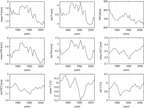
The three upper panels in Fig. 3 present the mean and standard deviation of daily precipitation and the mean number of wet days; the middle row presents the mean and standard deviation of precipitation during wet days and the mean of PET; and the bottom row presents the standard deviation of PET and the mean and standard deviation of daily air temperature.

As some of the indices are interrelated, their temporal variability is similar. In particular, there is a similarity between panels in the first row corresponding to precipitation, and between panels in the third row related to PET and air temperature. The results for the Axe catchment shown in Fig. 3 are characterized by a decline in the mean and standard deviation of precipitation and the number of wet days (first row), a lack of statistically-significant changes, assessed by the modified Mann-Kendall test (Hamed and Rao 1998), in the mean and standard deviation of precipitation during these days (second row), and a decrease of mean temperature (third row).

Similar analyses were carried out for the three other catchments, Kamp, Wieprz and Wimmera. The variability of climatic conditions in these catchments is presented in the Supplementary material.

4.2 HBV model calibration and validation

A summary of the calibration results is given in Table 4. The number of sub-periods varies from 24 for the Wieprz catchment to 38 for the Wimmera catchment. The Kling-Gupta efficiency (KGE) values (Gupta et al. 2009) illustrate the performance of the models during the calibration and validation stages. A sum of squared errors was applied as an objective function during the calibration stage, but derived from it, the KGE measure is more suitable for the comparison between the catchments. We also present results of the KGE decomposition into the linear correlation coefficient(r), a measure of relative variability in the simulated and observed time series (α), and the ratio between the mean simulated and observed values (β):

Table 4 Summary of the data length, number of sub-periods, and calibration and validation results of the HBV model for the four catchments. The values show the minimum, median and maximum values of the Kling-Gupta efficiency criterion and its decomposition into r: the linear correlation coefficient, α: a measure of relative variability in the simulated and observed time series, and β: the ratio between the mean simulated and observed values for the calibration and validation in a 5-year moving window.

		Axe	Kamp	Wieprz	Wimmera
Start of period		1 Jan. 1973	1 Jan. 1976	1 Nov. 1965	2 Jan. 1965
End of period		13 Dec. 2011	30 Dec. 2008	31 Dec. 1995	31 Aug. 2009
No. of sub-periods		33	28	24	38
Calibration
KGE	Min	−1.795	0.632	0.149	0.473
	median	0.507	0.832	0.567	0.769
	Max	0.711	0.897	0.909	0.868
r	Min	0.173	0.740	0.237	0.687
	median	0.785	0.856	0.671	0.900
	Max	0.859	0.929	0.922	0.931
α	Min	0.304	0.727	0.458	0.662
	median	0.803	0.924	0.753	0.863
	Max	0.855	1.007	0.972	0.960
β	Min	1.102	0.920	0.866	0.862
	median	1.407	0.967	0.931	1.143
	Max	3.577	1.013	0.978	1.391
Validation
KGE	Min	−14.917	−0.105	−0.678	−5.117
	Median	0.498	0.713	0.369	0.650
	max	0.759	0.911	0.893	0.899
r	Min	0.186	0.525	−0.415	0.455
	Median	0.742	0.786	0.574	0.859
	max	0.848	0.915	0.911	0.921
α	Min	0.157	0.462	0.187	0.360
	Median	0.799	0.942	0.641	0.940
	max	2.286	2.076	1.924	3.941
β	Min	0.333	0.800	0.561	0.492
	Median	1.230	0.967	0.943	1.185
	max	16.895	1.173	1.490	6.768

(5)

(6)

where subscripts s and o denote simulated and observed time series.

This decomposition allows for the detection of the main sources of problems during calibration. Good calibration results are required to derive potentially good parameter values and their robustness is assessed in the validation stage. In the ideal case, the three components of decomposed KGE are r = 1, α = 1 and β = 1. The results of decomposition show that the α values in the calibration period are always below 1, i.e. the variability is systematically underestimated (Gupta et al. 2009). This could be overcome when optimizing on KGE. The minimum KGE values for the calibration vary from −1.795 for the Axe catchment to 0.632 for the Kamp catchment. The poor results of the HBV model calibration are not due to problems with the optimization method, because in all cases (for all catchments and all sub-periods) convergence was reached. We tested whether the obtained values of an objective function strongly depend on climatic conditions. Our analysis indicates that KGE values are correlated with most of the analysed climatic characteristics. These correlations are statistically significant at the 0.05 level of confidence. The highest Pearson correlation values are estimated for mean precipitation. Figure 4 presents the relationships between mean precipitation and KGE values for the Axe, Kamp, Wieprz and Wimmera catchments. The worst calibration results are obtained for cases of very low mean precipitation in all four catchments. That outcome indicates that poor calibration and poor model performance are related to the low mean precipitation prevailing in those periods. It also indicates that it is more complex to model rainfall–runoff transformations under dry conditions.

Fig. 4 Scatterplots showing the relationship between mean precipitation and the KGE values obtained at the calibration stage for the Axe, Kamp, Wieprz and Wimmera catchments.

As a result of the SCEM-UA optimization method, the posterior distributions of the analysed parameters were estimated. The derived posteriors for most parameters exhibit an approximately normal distribution.

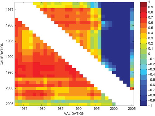
The second step was the validation of the derived models. For each calibration sub-period the optimized parameter set (corresponding to median parameter values from the posteriors) was used to perform all possible validations on the other sub-periods. The results of the validation depend on the catchment and the period (see the Table 4). The results of the model validation for the Axe catchment are shown in Fig. 5. The y-axis shows the start of the period for which the model is calibrated and the x-axis shows the start of the validation period. The obtained values of KGE range from −14.917 to 0.759. Figure 5 is set in a colour scale (−1 to 1), therefore all the KGE values below −1 are dark blue. We excluded the four neighbouring periods from the analysis due to data overlap. The worst results are obtained for the model calibrated on the period 1973–1978 and validated on the period 2004–2009. A comparison of climatic indices in these two periods indicates significant changes in precipitation (28.7% decrease of mean precipitation, 15.8% decrease of std P and decrease of number of wet days from 815 to 632 days). The differences in the other climatic indices are smaller than 10%.

Fig. 5 Validation results for the Axe catchment (values of KGE). Each row represents the KGE values for the validation of the model calibrated on the column year described by the x-axis. The obtained values of KGE range from −14 to 1, and are represented in colour. from blue (−14) to red (1). The figure is set in the colour scale (−1 to 1) and therefore all KGE values below −1 are dark blue.

The results for the three remaining catchments (Kamp, Wieprz and Wimmera) are presented in the Supplementary material.

The validation results illustrate typical patterns for the analysed catchments. All the analysed catchments are characterized by the existence of two periods with opposite (good and poor) results in the validation stage. Referring to climatic variability for the Axe catchment (Fig. 5) we note that the models calibrated on dry periods give poor performance during the wet periods. These results confirm the findings of Vaze et al. (2010), Merz et al. (2011) and Coron et al. (2012).

4.3 Temporal variability of HBV model parameters

The posterior distributions of the HBV model parameters are used to estimate the median and standard deviation of the obtained parameters for each catchment and each 5-year period.

The temporal variability of the HBV model parameters and its uncertainty for the Axe catchment are shown in Fig. 6. The results for the remaining three catchments (Kamp, Wieprz and Wimmera) are presented in the Supplementary material.

Fig. 6 Temporal variability of HBV model parameters for the Axe catchment. The dots represent the median values and whiskers represent 95% confidence limits.

Each panel in Fig. 6 presents the median and 95% confidence limits of six model parameters (FC, β, LP, α, KF and PERC) obtained for a 5-year moving window. It is worth noting that the median parameter values vary over wide ranges. The estimated confidence limits of the HBV model parameters are also varying with time. For the Axe catchment the widest confidence limits were estimated for the most recent periods with relatively dry climatic conditions.

4.4 Dependence of model parameters on climatic indices

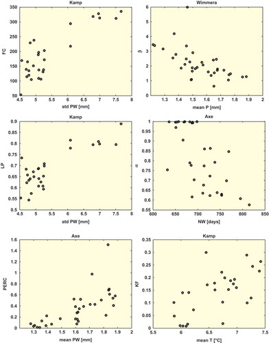
In the next step we estimated the dependence of the HBV model parameters on climatic indices using the Pearson correlation coefficient (PCC) and the weighted PCC (WPCC). An example of scatterplots with statistically significant relationships between the estimated HBV parameters and climatic characteristics for selected catchments (the Axe, Kamp and Wimmera) are shown in Fig. 7.

Fig. 7 An example of scatterplots showing statistically-significant relationship between the HBV model parameters and climatic indices for selected catchments.

The FC parameter has a significant influence on objective function values in all analysed catchments. The dependence of the median of the FC parameter on climatic indices is presented in Fig. 8. The derived PCCs are significant at the 0.05 level for three catchments: Axe, Kamp and Wimmera. The Wieprz catchment shows no statistically-significant correlation between the FC parameter and climatic indices.

Fig. 8 Statistically-significant Pearson correlation coefficient (PCC) between the FC parameter and climatic indices.

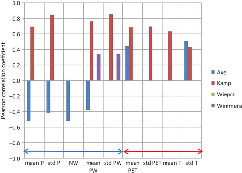
In order to take into account uncertainty of model parameters, the weighted Pearson correlation coefficient (WPCC) was calculated. The resulting WPCC values for the FC parameter are shown in the upper left panel of Fig. 9. The correlation between FC and water-dependent indices is statistically significant for two catchments (Kamp and Wieprz). In both cases the WPCCs take positive values except for NW for the Wieprz catchment.

Fig. 9 Statistically significant weighted Pearson correlation coefficient (WPCC) between parameters: FC, β, LP, α, KF, PERC, TT and CFMAX and climatic indices.

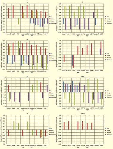
The values of WPCC for temperature-related climatic indices permit a classification of catchments into two groups. In the first group (Axe and Wimmera catchments) the values of WPCC are negative, which means that the FC parameter decreases when air temperature increases in these catchments. For the second group, the Kamp and Wieprz catchments, the WPCCs are positive and the FC parameter increases with an increase of air temperature (i.e. the soil moisture capacity increases). The Kamp and Wieprz catchments are located in the central part of Europe (Austria and Poland, respectively) and have similar climatic conditions. Therefore, we infer that these differences in the sign of WPCC values are most likely due to differences in climatic conditions. These results confirm the findings of Merz et al. (2011), where a positive Spearman rank correlation coefficient was found between the FC parameter and mean annual precipitation, temperature and evapotranspiration.

The FC parameter is a soil-related property (type, porosity, depth) and its values may also vary in response to the variability of climatic conditions (Merz et al. 2011). A higher temperature or observed PET will lead to a larger soil moisture storage capacity and smaller soil moisture deficit. The opposite tendency is visible with water-dependent indices; the more intense or longer precipitation, the lower the soil moisture deficit. Such a relationship is visible only in catchments without snow cover (Axe and Wimmera). In catchments located in cold climates the process of snow accumulation causes significant delays in the transition between precipitation and flow, resulting in the positive correlation between the FC parameter and water related indices. Such a situation can be seen in the Kamp and Wieprz catchments in Central Europe.

A comparison of the PCCs and WPCCs calculated for the FC parameter is presented in the upper left panel of Fig. 10. For the Kamp catchment PCCs and WPCCs take almost the same values. This results from very small uncertainty of the FC parameter. A comparison of the PCCs and WPCCs for the Wieprz catchment indicates that the calculated PCC values are not statistically significant, whilst the correlation estimated for the series with their uncertainty taken into account is statistically significant.

Fig. 10 A comparison of PCCs and WPCCs estimated for the FC, β, LP, α, KF, PERC, TT and CFMAX parameters in the Axe, Kamp, Wieprz and Wimmera catchments.

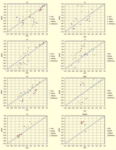
Taking into account the uncertainty of the HBV parameters can increase their estimated correlation with climatic indices as seen, for example, for the Axe and Wimmera catchments.

Similar analysis was performed for all other sensitive parameters of the HBV model: β, LP, α, KF, PERC, TT and CFMAX. The results of the analyses of the dependence of these parameters on climatic characteristics with parametric uncertainty taken into account are presented in Fig. 9. A comparison of estimated PCCs and WPCCs is shown in the remaining seven panels of Fig. 10. The results confirm the large influence of parametric uncertainty on the correlation between those parameters and climatic indices, varying with the catchment.

4.5 Summary of estimated dependencies

The results of dependence of the correlation analysis taking into account parametric uncertainty are summarized in Table 5.

Table 5 Number of catchments with statistically significant WPCC (positive or negative) vs number of cases, illustrating the correlation of the HBV parameter with climatic indices.

	FC	β	LP	α	KF	PERC	TT	CFMAX
Mean P	1/4	3/3	3/4	1/4	3/4	3/3	1/2	1/1
Std P	1/4	2/3	3/4	0/4	1/4	3/3	1/2	1/1
NW	1/4	2/3	2/4	2/4	1/4	3/3	1/2	0/1
Mean PW	2/4	3/3	4/4	1/4	0/4	2/3	1/2	1/1
Std PW	1/4	2/3	3/4	1/4	1/4	2/3	1/2	1/1
Mean PET	4/4	1/3	3/4	1/4	1/4	2/3	1/2	1/1
Std PET	4/4	1/3	3/4	1/4	1/4	2/3	1/2	1/1
Mean T	3/4	2/3	3/4	0/4	2/4	2/3	2/2	0/1
Std T	3/4	1/3	3/4	2/4	1/4	3/3	1/2	0/1

The WPCC analysis has a qualitative value, as only the first-order dependencies are estimated. However, we can draw some general conclusions from Table 5. The highest number of catchments with statistically significant WPCC is estimated for six cases: (a) FC parameter with mean PET and std PET, (b) β parameter with mean P and mean PW, (c) LP parameter with mean PW, (d) PERC parameter with mean P, std P, number of wet days and std T, (e) TT parameter with mean T, and (f) CFMAX parameter with mean P, std P, mean PW, std PW, mean PET and std PET.

Generalization of these relationships is impossible due to the very small sample and the large variability in the geographical and climatic conditions in the catchments. However, some patterns in the HBV parameter behaviour related to changes of climatic conditions can be discerned.

The FC parameter shows the most consistent dependency on temperature-related indices (mean PET, std PET, mean T and std T), having a significant correlation for most of the catchments. The correlation between FC and water-related indices occurs less frequently than the temperature-related indices. The parameter β shows a consistent dependence on water-related indices with less frequent correlation with temperature-related indices. Less frequent correlations are found for the α and KF parameters.

Considering the results from the perspective of the indices (rows in Table 5), the mean P shows the largest influence on the parameters (β, LP, KF, PERC, TT and CFMAX). The second most influential index is the mean PW, with frequent correlations with FC, β, LP, PERC, TT and CFMAX. For the temperature-related indices, correlation is most frequent for the mean PET and the standard deviation of PET.

5 CONCLUSIONS

This work was stimulated by a project aiming at the analysis of the nonstationarity of hydrological model parameters under varying conditions (Thirel et al. 2015). In the framework of that project, a common hydrometeorological database with data from 14 catchments was provided and the project participants tested the application of hydrological models under changing conditions for various time periods. This study is limited to four catchments, with the most stable land-use conditions, availability of input data and suitable for modelling with HBV.

The dependence of HBV model parameters on climatic indices was assessed using a 5-year moving window calibration by the SCEM-UA optimization method, carried out for four catchments in Europe and Australia. The robustness of the calibration was tested using cross-validation. The validation results illustrate a typical pattern for the analysed catchments. All four catchments are characterized by the existence of periods with good and weak results in the validation stage, which coincide with temporal variability of climatic indices.

The Pearson correlation coefficient (PCC) and its weighted version (WPCC) were used to test the dependence of model parameters on climatic indices. The WPCC allows for an analysis of the influence of HBV model parametric uncertainty on the derived correlations. The HBV model parametric uncertainty significantly influences the estimated correlations. In the case of large parameter uncertainty, the estimated PCCs are biased.

Most parameters show a statistically significant dependence on several climatic indices for all catchments but it is difficult to distinguish any specific patterns of dependence. Both the indices and HBV model parameters are correlated (Romanowicz et al. 2013). Therefore, the PCC and WPCC correlation analyses have only a qualitative value. However, we can draw some general conclusions. The FC parameter shows the most consistent dependence on temperature-related indices (mean PET, std PET, mean T and std T), having a significant correlation for all the analysed catchments. The correlation between FC and water-related indices is less strong in comparison with temperature-related indices. Parameter β shows a consistent dependence on water-related indices with less frequent correlation with temperature-related indices. The α and KF parameters show weak correlations with climatic indices.

The analysis indicates that mean P shows the largest influence on the HBV model parameters (β, LP, KF, PERC, TT and CFMAX). The second most influential climate index is mean PW, showing frequent correlations with FC, β, LP, PERC, TT and CFMAX. Among the temperature-related indices, mean PET and std PET show the largest correlation with the HBV model parameters.

Disclosure statement

No potential conflict of interest was reported by the author(s).

Supplementary material

Supplementary material for this article can be accessed at: http://dx.doi.org/10.1080/02626667.2014.967694.

Acknowledgement

The authors thank the reviewers (Thibault Mathevet, Harald Kling and Guillaume Thirel) for their constructive comments that helped to improve quality of the paper and to clarify the text.

Additional information

Funding

This work was partly financed by the project “Stochastic flood forecasting system (River Vistula reach from Zawichost to Warsaw)”, Institute of Geophysics, Polish Academy of Sciences, NSC contract no. 2011/01/B/ST10/06866.

REFERENCES

- Abebe, N.A., Ogden, F.L., and Pradhan, N.R., 2010. Sensitivity and uncertainty analysis of the conceptual HBV rainfall–runoff model: implications for parameter estimation. Journal of Hydrology, 389, 301–310. doi:10.1016/j.jhydrol.2010.06.007
- Akhtar, M., Ahmad, N., and Booij, M.J., 2008. The impact of climate change on the water resources of Hindukush-Karakorum-Himalaya region under different glacier coverage scenarios. Journal of Hydrology, 355, 148–163. doi:10.1016/j.jhydrol.2008.03.015
- Andréasson, J., et al., 2004. Hydrological change—climate change impact simulations for Sweden. Ambio, 33 (4), 228–234.
- Arheimer, B., Lindström, G., and Olsson, J., 2011. A systematic review of sensitivities in the Swedish flood-forecasting system. Atmospheric Research, 100, 275–284. doi:10.1016/j.atmosres.2010.09.013
- Bergström, S., 1995. The HBV model. In: V.P. Singh, ed. Computer models of watershed hydrology. Highlands Ranch, CO: Water Resources Publications, 443–476.
- Bergström, S., et al., 2001. Climate change impacts on runoff in Sweden—assessments by global climate models, dynamical downscaling and hydrological modelling. Climate Research, 16 (2), 101–112. doi:10.3354/cr016101
- Beven, K., 2006. A manifesto for the equifinality thesis. Journal of Hydrology, 320 (1–2), 18–36. doi:10.1016/j.jhydrol.2005.07.007
- Blöschl, G., Reszler, C., and Komma, J., 2008. A spatially distributed flash flood forecasting model. Environmental Modelling & Software, 23 (4), 464–478. doi:10.1016/j.envsoft.2007.06.010
- Booij, M.J., 2005. Impact of climate change on river flooding assessed with different spatial model resolutions. Journal of Hydrology, 303, 176–198. doi:10.1016/j.jhydrol.2004.07.013
- Booij, M.J. and Krol, M.S., 2010. Balance between calibration objectives in a conceptual hydrological model. Hydrological Sciences Journal, 55, 1017–1032. doi:10.1080/02626667.2010.505892
- Campolongo, F., Cariboni, J., and Saltelli, A., 2007. An effective screening design for sensitivity analysis of large models. Environmental Modelling and Software, 22, 1509–1518. doi:10.1016/j.envsoft.2006.10.004
- Christensen, J.H., et al., 2013. Climate phenomena and their relevance for future regional climate change supplementary material. In: T.F. Stocker, et al., eds. Climate change 2013: the physical science basis [online]. Contribution of Working Group I to the Fifth Assessment Report of the Intergovernmental Panel on Climate Change. Available from: http://www.climatechange2013.org and http://www.ipcc.ch [Accessed 29 April 2015].
- Cloke, H.L., et al., 2013. Modelling climate impact on floods with ensemble climate projections. Quarterly Journal of the Royal Meteorological Society, 139, 282–297. doi:10.1002/qj.1998
- Coron, L., et al., 2012. Crash testing hydrological models in contrasted climate conditions: an experiment on 216 Australian catchments. Water Resources Research, 48, W05552. doi:10.1029/2011WR011721
- Deckers, D.L.E.H., et al., 2010. Catchment variability and parameter estimation in multi-objective regionalisation of a rainfall-runoff model. Water Resources Management, 24, 3961–3985. doi:10.1007/s11269-010-9642-8
- Demirel, M.C., Booij, M.J., and Hoekstra, A.Y., 2013. Impacts of climate change on the seasonality of low flows in 134 catchments in the River Rhine basin using an ensemble of bias-corrected regional climate simulations. Hydrology and Earth System Sciences, 17, 4241–4257. doi:10.5194/hess-17-4241-2013
- Graham, L.P., Andréasson, J., and Carlsson, B., 2007. Assessing climate change impacts on hydrology from an ensemble of regional climate models, model scales and linking methods—a case study on the Lule River basin. Climatic Change, 81 (S1), 293–307. doi:10.1007/s10584-006-9215-2
- Gupta, H.V., et al., 2009. Decomposition of the mean squared error and NSE performance criteria: implications for improving hydrological modelling. Journal of Hydrology, 377, 80–91. doi:10.1016/j.jhydrol.2009.08.003
- Hamed, K.H. and Rao, A.R., 1998. A modified Mann-Kendall trend test for autocorrelated data. Journal of Hydrology, 204, 182–196. doi:10.1016/S0022-1694(97)00125-X
- Hamon, W.R., 1961. Estimation potential evapotranspiration. Journal of the Hydraulics Division, Proceedings of the ASCE, 87 (HY3), 107–120.
- IPCC (Intergovernmental Panel on Climate change), 2013. Climate change 2013: The physical science basis [online]. Contribution of Working Group I to the Fifth Assessment Report of the Intergovernmental Panel on Climate Change. Cambridge: Cambridge University Press. Available from: http://www.ipcc.ch/ [Accessed 29 April 2015].
- Komma, J., et al., 2007. Ensemble prediction of floods—catchment non-linearity and forecast probabilities. Natural Hazards and Earth System Sciences, 7, 431–444. doi:10.5194/nhess-7-431-2007
- Li, C.Z., et al., 2012. The transferability of hydrological models under nonstationary climatic conditions. Hydrology and Earth System Sciences, 16, 1239–1254. doi:10.5194/hess-16-1239-2012
- Lindström, G., 1997. A simple automatic calibration routine for the HBV model. Nordic Hydrology, 28 (3), 153–168.
- Lindström, G., et al., 1997. Development and test of the distributed HBV-96 hydrological model. Journal of Hydrology, 201 (1–4), 272–288. doi:10.1016/S0022-1694(97)00041-3
- Merz, R., Parajka, J., and Blöschl, G., 2011. Time stability of catchment model parameters: implications for climate impact analyses. Water Resources Research, 47, W02531. doi:10.1029/2010WR009505
- Morris, M.D., 1991. Factorial sampling plans for preliminary computational experiments. Technometrics, 33, 161–174. doi:10.1080/00401706.1991.10484804
- Nash, J.E. and Sutcliffe, J.V., 1970. River flow forecasting through conceptual models. Part I—a discussion of principles. Journal of Hydrology, 10 (3), 282–290. doi:10.1016/0022-1694(70)90255-6
- Olsson, J. and Lindström, G., 2008. Evaluation and calibration of operational hydrological ensemble forecasts in Sweden. Journal of Hydrology, 350, 14–24. doi:10.1016/j.jhydrol.2007.11.010
- Parajka, J., Blöschl, G., and Merz, R., 2007. Regional calibration of catchment models: potential for ungauged catchments. Water Resources Research, 43, W06406. doi:10.1029/2006WR005271.
- Potter, N.J. and Chiew, F.H.S., 2011. An investigation into changes in climate characteristics causing the recent very low runoff in the southern Murray-Darling Basin using rainfall-runoff models. Water Resources Research, 47, W00G10. doi:10.1029/2010WR010333
- Pozzi, F., Di Matteo, T., and Aste, T., 2012. Exponential smoothing weighted correlations. European Physical Journal B, 85 (6), Article 175. doi:10.1140/epjb/e2012-20697-x
- Reszler, C., Blöschl, G., and Komma, J., 2008. Identifying runoff routing parameters for operational flood forecasting in small to medium sized catchments. Hydrological Sciences Journal, 53 (1), 112–129. doi:10.1623/hysj.53.1.112
- Romanowicz, R.J., Osuch, M., and Grabowiecka, M., 2013. On the choice of calibration periods and objective functions: a practical guide to model parameter identification. Acta Geophysica, 61 (6), 1477–1503. doi:10.2478/s11600-013-0157-6
- Schweppe, F.C., 1973. Uncertain dynamic systems. Upper Saddle River, NJ: Prentice-Hall.
- Seibert, J., 1999. Regionalisation of parameters for a conceptual rainfall-runoff model. Agricultural and Forest Meteorology, 98–99, 279–293. doi:10.1016/S0168-1923(99)00105-7
- Seibert, J., 2003. Reliability of model predictions outside calibration conditions. Nordic Hydrology, 34, 477–492.
- Singh, R., et al., 2011. A trading-space-for-time approach to probabilistic continuous streamflow predictions in a changing climate—accounting for changing watershed behavior. Hydrology and Earth System Sciences, 15, 3591–3603. doi:10.5194/hess-15-3591-2011
- Sorooshian, S. and Gupta, V.K., 1983. Automatic calibration of conceptual rainfall-runoff models: the question of parameter observability and uniqueness. Water Resources Research, 19 (1), 260–268. doi:10.1029/WR019i001p00260
- Thirel, G., et al., 2015. Hydrology under change: an evaluation protocol to investigate how hydrological models deal with changing catchments. Hydrological Sciences Journal, 60 (7–8), doi:10.1080/02626667.2014.967248
- Van Pelt, S.C., et al., 2009. Discharge simulations performed with a hydrological model using bias corrected regional climate model input. Hydrology and Earth System Sciences, 13, 2387–2397. doi:10.5194/hess-13-2387-2009
- Van Werkhoven, K., et al., 2008. Characterization of watershed model behavior across a hydroclimatic gradient. Water Resources Research, 44, W01429.
- Vaze, J., et al., 2011. Rainfall-runoff modelling across southeast Australia: datasets, models and results. Australian Journal of Water Resources, 14, 101–116.
- Vaze, J., et al., 2010. Climate nonstationarity—validity of calibrated rainfall-runoff models for use in climate change studies. Journal of Hydrology, 394, 447–457. doi:10.1016/j.jhydrol.2010.09.018
- Vrugt, J.A., et al., 2003. A shuffled complex evolution metropolis algorithm for optimization and uncertainty assessment of hydrologic model parameters. Water Resources Research, 39 (8), 1201. doi:10.1029/2002WR001642
- Vrugt, J.A., et al., 2006. Application of stochastic parameter optimization to the sacramento soil moisture accounting model. Journal of Hydrology, 325 (1–4), 288–307. doi:10.1016/j.jhydrol.2005.10.041
- Wilcox, R.R., 2005. Introduction to robust estimation and hypothesis testing. New York: Academic Press.