Hydrological modelling of temporally-varying catchments: facets of change and the value of information

Abstract

River basins are by definition temporally-varying systems: changes are apparent at every temporal scale, in terms of changing meteorological inputs and catchment characteristics due to inherently uncertain natural processes and anthropogenic interventions. In an operational context, the ultimate goal of hydrological modelling is predicting responses of the basin under conditions that are similar or different to those observed in the past. Since water management studies require that anthropogenic effects are considered known and a long hypothetical period is simulated, the combined use of stochastic models, for generating the inputs, and deterministic models that also represent the human interventions in modified basins, is found to be a powerful approach for providing realistic and statistically consistent simulations (in terms of product moments and correlations, at multiple time scales, and long-term persistence). The proposed framework is investigated on the Ferson Creek basin (USA) that exhibits significantly growing urbanization during the last 30 years. Alternative deterministic modelling options include a lumped water balance model with one time-varying parameter and a semi-distributed scheme based on the concept of hydrological response units. Model inputs and errors are respectively represented through linear and nonlinear stochastic models. The resulting nonlinear stochastic framework maximizes the exploitation of the existing information by taking advantage of the calibration protocol used in this issue.

Résumé

Les bassins versants sont par définition des systèmes temporellement variables: des changements apparaissent à toutes les échelles de temps, en termes de forçages météorologiques ou de modifications des caractéristiques des bassins, respectivement dus à des processus naturels aléatoires ou à des interventions humaines. Dans un contexte opérationnel, le but ultime de la modélisation hydrologique est la prévision des réponses du bassin sous des conditions similaires ou différentes de celles observées dans le passé. Puisque les études sur la gestion de l’eau requièrent que les influences anthropiques soient considérées comme connues et qu’une longue période hypothétique soit simulée, l’utilisation combinée de modèles stochastiques, pour générer les forçages, et de modèles déterministes qui représentent l’intervention humaine sur la modification des bassins, s’est révélée performante pour fournir des simulations réalistes et statistiquement cohérentes (en termes de moments et de corrélations, selon de multiples échelles, ainsi qu’en termes de persistance à long terme). Ce cadre de travail a été mis en œuvre sur le bassin de Ferson Creek (USA) qui présente une urbanisation significativement croissante durant les 30 dernières années. Des options alternatives de modélisation déterministe ont été adoptées, incluant un modèle global de bilan en eau avec un paramètre variable au cours du temps et un schéma semi-distribué basé sur le concept des unités de réponse hydrologique. Les forçages et erreurs du modèle sont respectivement représentés par des modèles stochastiques linéaires et non-linéaires. La structure stochastique non-linéaire résultante maximise l’exploitation de l’information existante, en profitant du protocole de calage utilisé dans ce numéro spécial.

Key words:

• modified basins
• hydroclimatic variability
• model and parameter uncertainty
• statistical consistency
• Hurst-Kolmogorov dynamics
• hydrological response units
• error model
• stochastic simulation
• hybrid calibration
• nonlinear stochastic modelling

Mots clefs:

• bassins modifiés
• variabilité hydro-climatique
• incertitude du modèle des paramètres
• cohérence statistique
• dynamique de Hurst-Kolmogorov
• unités de réponse hydrologique
• erreur de modèlisation
• simulation stochastique
• calage hybride
• modélisation stochastique non-linéaire

1 INTRODUCTION

Change is intrinsic in natural systems. In hydrological systems particularly, change is present at all temporal scales, and is reflected in both the short- and long-term variability of the observed states and fluxes (Koutsoyiannis 2013). Actually, this variability is manifested not exclusively in the system processes (i.e. input, output and state variables) but also in its properties (i.e. physical characteristics), which are changing over time. In this context, catchments should always be handled as temporally-variable systems. In fact, according to the new concept introduced within the “Panta Rhei” initiative, river basins are considered as the “changing interface between environment and society” (Montanari et al. 2013). This accounts for both systematic and non-systematic changes, respectively referring to stationary stochastic processes and deterministic time evolution. In general, systematic changes are prone to some kind of deterministic mathematical description, in as far as they are recognizable and relatively easy to interpret. For instance, major anthropogenic interventions by means of large-scale hydraulic structures (e.g. dams) obviously result in permanent modifications of the hydrological regime of a river basin. For this reason, such catchments are usually referred to as human-modified, and they can be comprehensively represented through effective coupling of hydrological and water management models (Nalbantis et al. 2011). Systematic changes may also be observable in the land-cover characteristics of the catchment, due to deforestation, urbanization or change of agricultural practices. However, an explanation of the overall changing behaviour of the catchment, which would allow the prediction of its responses in the long run, is still far from feasible.

Usually, catchments are modelled through nonlinear deterministic approaches, aiming to establish simplified cause–effect relationships between the varying inputs (e.g. precipitation, temperature) and the associated responses. In this context, the model parameters, representing catchment properties in an abstract sense, are considered as time invariant quantities. Under this premise, the observed variability of the simulated fluxes is expected to be explained by the variability of the hydrological inputs, to a large extent. Yet, in several cases, the deterministic models show unexpectedly poor performance, mainly because they underestimate the observed variability of the system responses. Such failure is typically attributed to data errors, improper parameterizations or non-robust calibrations (see Andréassian et al. 2010, Kuczera et al. 2010).

In fact, the improper representation of uncertainty is an intrinsic drawback of deterministic hydrological models, since these are not equipped with tools enabling the preservation of the associated statistical characteristics of the historical data (Efstratiadis 2011). In general, as the result of their simplified structure (e.g. representation of complex regulating mechanisms through linear reservoirs), models provide smoother responses than real-world systems. This structural deficiency will here be referred to as the model uncertainty, which is quantified in terms of error measures between the observed and simulated fluxes (e.g. the Nash-Sutcliffe efficiency, NSE). Modelling is generally aimed to ensure the minimum model uncertainty, through the most parsimonious parameterization. This task is not straightforward, given that more complex schemes tend to provide smaller errors in calibration, due to over-fitting. However, a large number of parameters, if they are poorly constrained by the available information, can result in considerable variability and associated parameter uncertainty (Hrachowitz et al. 2013). In order to simultaneously reduce model and parameter uncertainty, it is essential to maximize the information embedded in calibration, e.g. through using multicriteria approaches (Efstratiadis and Koutsoyiannis 2010), as well as ensuring transposability of models in time, by optimizing their performance across different periods and under different hydroclimatic conditions (Andréassian et al. 2009). In this vein, Thirel et al. (2015) proposed a parameter estimation protocol for catchments under changing conditions, which accounts for multiple criteria and aims to provide ‘stable’ calibrations.

An alternative approach to simulate temporally-varying catchments is through stochastic simulation, typically based on linear stochastic processes. Here linearity refers to the mathematical representation of processes in terms of linear relationships (correlations) between variables in space and time. In contrast to the deterministic models, which are often designed to reproduce the expected value of the involved processes, stochastic models are by nature built to reproduce the essential statistical characteristics (at least those of a second order) of the observed processes, in an attempt to capture their total variability, as this is reflected in the related observations. We note that in stochastic theory, change is not synonymous with non-stationarity, which has been widely used in recent years to denote all irregular variations of hydrometeorological processes (e.g. trends). Quoting Koutsoyiannis (2011), stochastic models hypothesizing stationarity but in parallel admitting a scaling behaviour (the so-called Hurst-Kolmogorov dynamics) can adequately describe “even prominent changes, at a multitude of time scales”. Hence, stochastic models handle change from a macroscopic (i.e. statistical) point of view, without accounting for its individual components (and causes). However, in the case of systematic and feasible-to-quantify changes that are embedded in the historical data, while not representative of future conditions, stochastic approaches that do not explicitly consider catchment dynamics will most likely lead to overestimation of uncertainty. Therefore, stochastic modelling of this type of catchment response, based on historical data under temporally-varying conditions, may result in erroneous decisions, due to misleading statistical information in these data.

It becomes evident that the incorporation of stochastic components in deterministic models can significantly improve the estimation of uncertainty in temporally-varying catchments. In this context, residual error components are embedded in some hydrological models, which enable, among others, the specification of confidence intervals of the simulated responses (yet, in this case, the models are no longer purely deterministic). Uncertainty estimations are also improved when deterministic models are combined with stochastic generators of meteorological inputs. Such approaches have been mainly reported in continuous flood simulation applications, in which what is asked is to estimate extreme probabilistic quantities (e.g. Franchini et al. 2000, Kuchment and Gelfan 2002, Blazkova and Beven 2004, Fiorentino et al. 2007, Gelfan 2010). Deterministic hydrological models fed by stochastic inputs are also used in the context of water management studies (e.g. Nalbantis et al. 2011). Yet, none of the above approaches can guarantee full exploitation of the statistical information contained in the historical data, combined with knowledge about recent or expected modifications of the basin characteristics.

In this paper we propose an integrated stochastic-deterministic modelling framework for distinguishing between uncertainty due to systematic changes and uncertainty attributed to other causes, including non-systematic facets of change. Within this framework, change is considered as the apparent effect of varying meteorological inputs on catchments with time-varying characteristics. Part of this change is assumed to be known and is explicitly accounted for in simulations. By coupling the two classical modelling approaches we wish to take advantage of the physical consistency of deterministic hydrological models and the statistical consistency of the linear stochastic models. The result of this coupling is in effect a stochastic model, but not a linear one. The nonlinearity of the combined approach, induced by the deterministic model, allows for a more faithful representation of the catchment behaviour and provides a better basis to exploit the available information, while the stochastic output is an advantage over the single output of the deterministic approach. The proposed framework is applicable for long-term simulations accepting stationarity of input processes and steady-state basin properties, and is in harmony with the recently proposed theoretical scheme by Montanari and Koutsoyiannis (2012); see also Sikorska et al. (2014), although the latter is more suitable for short-term predictions, based on synthetically generated ensembles.

The methodology is tested in an urbanized catchment in the USA (Ferson Creek), for which we initially employ three alternative deterministic modelling schemes. Their calibration is based on a hybrid (i.e. manual and automatic) calibration procedure. In order to check the acceptability of each model, we follow the protocol of Thirel et al. (2015), which assists the detection of robust parameter sets. The most appropriate of the deterministic modelling schemes is then coupled with two stochastic models, one for the generation of model inputs and the other for the model errors, thus formulating a nonlinear stochastic scheme. This scheme is employed in stochastic simulation mode, considering three different sources of uncertainty: (a) hydroclimatic uncertainty, by means of variability of input processes (precipitation, temperature); (b) model uncertainty, by means of variability of model residuals; and (c) changes induced by urbanization, by means of scenarios for steady-state urban development. Within this approach, two kinds of ‘hard-type’ information are explicitly accounted for, namely systematic hydrological observations and sparse data of urban development, for a 32-year period. In addition, hydrological experience holds a key role in all aspects of the proposed framework, which can be viewed as ‘soft-type’ information.

2 THE NONLINEAR STOCHASTIC MODELLING FRAMEWORK

2.1 Questions to be answered

As stressed in the Introduction, we focus on model use for solving water management problems. Such problems include the planning, design and operation of man-made components of hydrosystems. By restricting our scope to medium-term problems, we fix the future time horizon to a few years ahead. Daily flow availability at that time will be estimated, which correctly reflects meteorological variability. Although the basin under study will be temporally-varying in historical time, such variability is undesirable when studying future basin responses. What is sought is the response of the basin under a future steady state of its properties. Scenarios of the basin state will provide a rational basis for predicting the basin response (i.e. daily runoff) under upper, mean and lower urban development states.

Herein, we set out to find the optimal modelling scheme by means of preserving the statistical behaviour (at multiple scales, from daily to over-annual) of the basin response under steady basin state, i.e. statistics reflecting the effect of meteorological input only. The modelling scheme is summarized in the following equation:

(1)

where y_t is the output vector at time t; DM(.,.) is the deterministic model with input vector x_t at time t and parameters θ; ٠ is an arithmetic operator (e.g. summation or multiplication); and ε_t is an error term. The input vector x_t will be generated through a linear stochastic modelling scheme described in Section 2.5, and the error term ε_t will be generated by the stochastic model described in 2.6.

The following questions arise:

1. How can the advantages of linear stochastic and nonlinear deterministic models be jointly exploited?

2. How can we effectively parameterize the deterministic model for the kind of change selected (i.e. growing urbanization)?

3. How can we ensure a satisfactory compromise between model and parameter uncertainty?

4. What is the gain of a nonlinear stochastic approach over a linear stochastic one?

5. What is the effect of ignoring the error (model uncertainty) of the deterministic model?

To answer the above questions, a number of deterministic models (DM of equation (1)) have been devised, or simply used, and are described next. The way the models are employed to address the above questions is presented in Section 2.7.

2.2 Lumped deterministic model without consideration of urbanization (DM0)

The hydrological processes are modelled through a lumped conceptual scheme that uses 11 parameters. The basin is vertically subdivided into three storage elements or tanks that represent the snowpack, soil water and groundwater (Fig. 1). Model inputs are daily precipitation, P, and mean daily temperature, T. Fluxes are expressed in units of water depth (i.e. mm) per unit time, while storages are water depths. The time interval of simulations is denoted as Δt (in the specific case, Δt = 1 d).

Fig. 1 Sketch of the conceptual model DM0, illustrating the modelled processes and associated parameters.

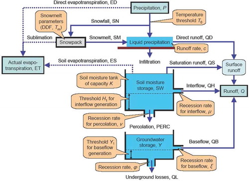
First, precipitation is considered as snowfall, SN, if T is below a certain threshold, T₀ (°C). In this case, potential evapotranspiration (PET) is considered as sublimation and has no further influence on soil water. In the opposite case, precipitation is considered to be liquid and fulfils, by priority, the potential evapotranspiration. The latter is estimated according to the empirical formula by Oudin et al. (2005):

(2)

where R_a is the extra-terrestrial radiation, which is a function of latitude and time within the year; λ is the latent heat of vaporization, with a typical value of 2460 kJ/kg; k₁ (°C) is a scale parameter; and k₂ (°C) is a parameter related to the threshold for air temperature, i.e. the minimum value of air temperature for which evapotranspiration is not zero. In the model we employ the generally recommended values k₁ = 100°C and k₂ = 5°C.

Snowfall and sublimation allow us to update the water equivalent of the snowpack tank via the snowpack water balance. Then, the snowmelt, SM, is estimated through the degree-day method as:

(3)

where DDF is the degree-day factor (mm/d/°C) and T_m is a temperature threshold (°C) above which snowmelt occurs.

A time-varying fraction of the liquid precipitation or snowmelt is assumed to contribute to direct runoff, QD, as:

(4)

where c is a dimensionless parameter, SW is the soil water storage and K (mm) is the associated capacity of the soil water tank. According to the above relationship, the runoff rate increases as the soil tank tends to saturation.

The remainder enters the soil water storage tank if there is enough empty space in it. Otherwise, saturation excess runoff, QS, is produced and is obtained as:

(5)

The soil water tank loses water through actual evapotranspiration, ES, as:

(6)

where, PET is potential evapotranspiration and H₁ is a threshold (mm).

The second loss is interflow, QH, which is a fraction, μ, of the soil water above the same threshold H₁ as above. The quantity μ acts as a recession parameter. Analytically:

(7)

Soil water is lost through percolation to groundwater, which is determined as the fraction, ν, of soil water storage (also acting as a recession parameter), i.e.:

(8)

The quantity PERC enters the groundwater storage tank that loses water through baseflow and lateral outflow to the downstream groundwater system. Baseflow, QB, is calculated as:

(9)

where ξ is a recession parameter, Y is the current groundwater storage and Y₁ is a threshold value. Similarly, underground losses are obtained as:

(10)

where φ is a recession parameter. All recession parameters (μ, ν, ξ, φ) are expressed in inverse time units (d⁻¹).

The total runoff Q is obtained by summing the four runoff components:

(11)

Finally, the water balance equations are used for the three tanks of the model.

2.3 Lumped deterministic model with consideration of urbanization (DM1)

All hydrological processes are represented in a manner identical to that of model DM0, with the exception of direct runoff. The latter is hypothesized to exclusively represent runoff from the urban impervious area, which, in turn, is assumed to linearly depend on the fraction of the urban area, f_U. The percentage of area of the rural impervious surface is assumed negligible, which is realistic in most watersheds of the temperate zone of the Earth, such as that used in our tests.

The above assumptions are mathematically expressed by considering parameter c of equation (4) as a constant fraction, θ, of the urban area fraction f_U. Analytically:

(12)

where f_U is given in the form of input time series.

2.4 Semi-distributed deterministic hydrological model (DM2)

The growing urbanization is taken into account by considering two hydrological response units (HRUs). The concept dates back to Flügel (1995), who proposed it to characterize homogeneous areas with similar geomorphologic and hydrodynamic properties. This is commonly defined as a spatial element of pre-determined geometry, following exactly the logic of the schematization of the basin. Recognizing that this leads to models with unnecessarily large number of parameters, Efstratiadis et al. (2008), in proposing their model known as Hydrogeios, defined the HRU as a partition of the basin corresponding to a specific class combination of basin properties, such as soil permeability, land cover, or terrain slope, not necessarily comprised of contiguous geographical areas.

In this model, the urbanization effect is assumed to be predominant with regard to spatial differences in the hydrological response within the studied basin. Due to the large urban fraction and its rapid growth, this assumption is expected to be realistic. Also, the contiguity of time-varying urban areas cannot be ascertained. Obviously, this led us to adopt the concept of two HRUs: the first (HRU 1) represents the time-varying (growing) urban area, while the second (HRU 2) corresponds to rural areas that are also time-varying (shrinking). At each HRU we implement the model DM0 up to equation (8), assuming common parameters for snow accumulation and snowmelt (DDF, T₀, T_m), as is logical, but different parameterization for the overland and soil processes. In particular, in urban areas the generation of direct runoff is considered as a constant fraction, c, of the sum of the available precipitation and snowmelt:

(13)

while in rural areas, QD is expressed as a nonlinear function of the actual soil moisture storage (equation 4). Similar to the process representation in rural areas, the remainding quantity, i.e. P + SM – QD, enters a soil moisture accumulation tank that lies underneath the urban area. Next, the other two components of surface runoff (i.e. overland flow due to saturation, QS, and interflow, QH), the actual evapotranspiration through the soil, ES, and the deep percolation, PERC, are estimated through equations (5)–(8), in which we assign different values for the storage (K, H₁) and recession (μ, ν) parameters.

In order to preserve parsimony, for the groundwater processes we follow a lumped approach, by employing equations (9)–(11) to a common groundwater tank. The latter is fed by a weighted sum of the percolations generated by the two distinct HRUs, as:

(14)

where PERC₁ and PERC₂ are the percolation depths from the urbanized (HRU 1) and rural areas (HRU 2), respectively.

The total runoff of the basin is calculated as:

(15)

where Q₁ and Q₂ are the surface runoff depth from the urbanized and rural areas, respectively, and QB is the baseflow depth, which is generated by the groundwater tank. Each of components Q₁ and Q₂ is equal to the sum of QD + QS + QH of the respective HRU.

This version of the model has 16 parameters. The five extra parameters with respect to those of DM0 and DM1 are associated with the hydrological processes in the urban HRU.

2.5 Linear stochastic modelling scheme for time series generation (LSM)

Stochastic simulation using synthetic data that represent non-deterministic inputs to a water resource system (e.g. precipitation, runoff, temperature) is a powerful technique that allows one to account for uncertainty of the related processes. The key concept is to provide a long time series of synthetic data, thus allowing the underlying simulation model of the system to be run for a long time horizon, in order to estimate its performance by statistical means (e.g. reliability, safe yield, risk), with satisfactory accuracy. This is of high importance, since the usually short length of historical data series is inadequate for estimation of the desired probabilistic performance indices. This option can be offered by synthetic data, whose statistics up to a certain order (usually the third order) are statistically equivalent to those of the observed data. Such consistency is ensured when the essential statistical properties of the historical time series are reproduced in the synthetic ones as closely as possible. According to the classical study by Matalas and Wallis (1976), these include the marginal statistics up to third order (mean, standard deviation, skewness) and the joint second-order statistics (autocorrelations and lag-zero cross-correlations). The preservation of the statistical characteristics should be ensured not only for the time scale of the parent historical data (i.e. the time resolution of simulation), but also for coarser scales. We emphasize that the preservation of the statistical characteristics merely at the finer temporal scale may result in significant underestimation of the uncertainty metrics (e.g. variance) at the coarser scales, including the long-term persistence (Hurst-Kolmogorov dynamics), which is a dominant facet of uncertainty at all temporal scales (Koutsoyiannis 2011). Typically, this problem (also referred to as ‘overdispersion’; see Katz and Parlange 1998) is tackled by disaggregation techniques, which allow proper representation of the different statistical behaviour of the simulated hydrometeorological processes across different temporal scales.

As explained in Section 2.7, in the context of our simulations we aim to generate daily time series of 1000-year length for three processes of interest, namely precipitation, temperature and runoff. In this vein, we use the enhanced version of the Castalia software, which is fully described in Efstratiadis et al. (2014). Castalia implements a three-level linear multivariate stochastic simulation scheme that preserves the aforementioned essential statistics at the daily, monthly and annual time scales. Moreover, it reproduces the long-term persistence (LTP) at the annual and over-annual scales, the periodicity at the monthly scale, and the intermittency at the daily scale, in terms of preserving the so-called ‘probability dry’ of the process of interest (‘probability dry’ is often used to denote the probability that the value of a hydrological process within a time interval is zero). Models are linear in the sense that only linear combinations of random variables appear in the model equations. The generation procedure is employed from the annual to monthly and then to the daily time scale, through subsequent disaggregation approaches, as follows:

First, the annual time series are generated through a symmetric moving average (SMA) scheme introduced by Koutsoyiannis (2000). SMA implements the generalized autocovariance function:

(16)

where γ_j is the autocovariance of the annual stochastic process for lag j; γ₀ is the variance; and κ, β are shape and scale parameters, respectively, that are related to the persistence of the simulated process. By adjusting the values of κ and β, one can take a wide range of feasible autocovariance structures, which enables the representation of processes from the ARMA-type to highly persistent ones. In order to reproduce LTP, the recommended (and default) value of the scale parameter is β = 2, while the shape parameter κ is conditioned by the observed lag-1 autocorrelation, ρ₁, defined as γ₁/γ₀.

For the monthly time scale, auxiliary time series are initially provided by a multivariate first-order autoregression scheme, PAR(1), the parameters of which are periodic (monthly) functions of time (Koutsoyiannis 1999). Next, a disaggregation approach is employed to establish statistical consistency between the monthly and annual temporal scales, using a linear adjusting procedure (Koutsoyiannis 2001).

The general approach for generating synthetic daily data resembles the case of monthly data, since auxiliary time series are initially produced through a PAR(1) model, and these are then adjusted to the known monthly values. However, the computational procedure is more complicated, given that, apart from the essential statistical characteristics that, similarly to monthly simulations, are periodic functions of time, it is also necessary to reproduce intermittency, i.e. the proportions of intervals with zero (or near-zero) values of the modelled variables. Thus, in the disaggregation context, we employ a proportional adjusting scheme, combined with hybrid rules for the preservation of intermittency, proposed by Koutsoyiannis et al. (2003).

2.6 Stochastic model for errors of deterministic hydrological models (EM)

In everyday practice, model errors of deterministic hydrological models are usually neglected and fluxes predicted or forecast via deterministic models are directly employed in water resources management studies. As mentioned in the Introduction (Section 1), the implementation of simplified storage–discharge relationships smoothes the flux signal (e.g. Suweis et al. 2010); this in turn creates biases in critical water management quantities that are estimated through models (e.g. the reservoir storage capacity required for fixed target release and reliability level). By defining model errors, e_t, as the differences between the observed and simulated fluxes, all sources of uncertainty are assumed to be embedded in them. For an ideal hydrological model, the following properties of error are desirable (e.g. Sorooshian and Dracup 1980): (a) the error is uncorrelated with the simulated runoff; (b) the error is uncorrelated with itself (zero autocorrelation); and (c) the error is an i.i.d. random variable, i.e. without periodicity or other kind of time variation in its statistical properties.

In this paper it is assumed that the third requirement is fulfilled and is only checked a posteriori on stochastic residual time series. Preliminary tests showed that requirements (a) and (b) are not fulfilled. To overcome this problem, we defined the transformed runoff:

(17)

where ε is a scale parameter, introduced to avoid zero flow values, that was set to 1% of the mean daily observed runoff (in this study, ε = 0.01 mm). The rationale of this transformation, which is related to the definition of entropy for non-negative variables and non-Euclidean measures, is explained in Koutsoyiannis (2014). Accordingly, the error process, w_t, non-dimensioned by ε, is:

(18)

where Q_t and Q_sim,t are the ‘true’ and simulated runoff at time t, respectively. The transformed errors are decorrelated from flows, while to obtain actual errors it suffices to use the inverse transformation.

The error processes, w_t, are still autocorrelated and a first-order autoregressive model, or AR(1), is used to model them. Low-order stationary autoregressive models are reported to have commonly been used as error models in the past (e.g. Nalbantis 2000). The model is applied in the form:

(19)

where w_t is the transformed error process defined by equation (18), with mean μ, standard deviation σ, skewness γ, and lag-1 autocorrelation coefficient ρ; φ₁ is the first-order autoregression coefficient; and z_t is a random process with mean μ_z, standard deviation σ_z, skewness coefficient γ_z, and zero autocorrelation. The statistical characteristics of the random process z_t are given by:

(20)

(21)

(22)

The parameters of the AR(1) model are estimated as follows:

• the residuals of the deterministic model (DM0, DM1 or DM2, where applicable) are obtained from equation (18), where the true runoff is replaced by the observed value;

• the essential statistics of these residuals are estimated, i.e. mean, , standard deviation, , skewness coefficient, , and lag-1 autocorrelation coefficient, ;

• the statistics of the random process are obtained through equations (19), (20) and (21), by replacing μ, σ, γ and ρ with their estimates, i.e. , , and , respectively.

The three-parameter gamma distribution is considered to represent the random process z_t. Its parameters (shape, scale and location) are estimated using the method of moments, as functions of , and .

Let Q_sim, t be a runoff process estimated through a deterministic modelling approach, without accounting for the error induced due to model uncertainty. Inverting equation (18) allows the calculation of the ‘true’ runoff, Q, in simulation mode as:

(23)

which is equivalent to considering an untransformed error:

(24)

Multiplicative errors of runoff similar to those of equation (24) are not new in hydrological research studies, but have also been used in the past (e.g. by Nalbantis et al. 1995).

2.7 Proposed modelling framework and the testing experiment

In Section 2.1 five research questions were posed. Responses to those questions required the formulation of a nonlinear stochastic modelling framework. The necessary steps to employ this framework to respond to the above questions form our testing experiment, which is described next.

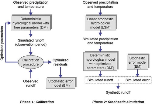
To respond to Question 1 we set up the combined deterministic-stochastic framework of Fig. 2. Two alternative deterministic models are used, namely DM1 and DM2 (described in Sections 2.3 and 2.4, respectively). These models have the advantage of exploiting information on the known systematic change of the test basin, i.e. urbanization. As explained in the Introduction, modelling the errors of deterministic models cannot be avoided for a wide spectrum of applications. For this reason, a stochastic error model (EM) for the errors of deterministic models was constructed, as described in Section 2.6. As also mentioned in our Introduction, the stochastic approach has the advantage of allowing the accurate estimation of probabilistic metrics or indices often required in water resources studies. This led us to add a second phase in our testing experiment, where the proposed modelling framework is fed with synthetically generated input data series to produce long series of model responses under a scenario of a constant level of urbanization. The tool to achieve this is the linear stochastic model (LSM) of Section 2.5. Within this phase, the error model is also used to generate model error sequences to be added to simulated responses from the deterministic models. The success or failure of the proposed modelling framework is evaluated based on the plausibility of model predictions in terms of statistics of the basin response at coarse time scales (monthly and annual).

Fig. 2 Outline of the nonlinear stochastic framework for hydrological modelling.

Question 2, referring to the effectiveness of deterministic model parameterization, is simple to address: It suffices to compare the performance of models DM1 and DM2 with each other and with the model that ignores urbanization, i.e. DM0.

Question 3 is mainly addressed at the calibration stage, which requires a strong hydrological background; therein, we seek a deterministic model with the least number of parameters such that the magnitude of the unexplained part of basin response variability reaches an acceptable level. A good equilibrium between model and parameter uncertainty is established by calibrating a number of deterministic models on observed data, until a model with fairly stable model performance is found. Performance stability (and, to a lesser degree, parameter stability) is checked using the protocol proposed by Thirel et al. (2015); the latter is based on the subdivision of the observation period into subsequent non-overlapping sub-periods and checking the differences of model performance (by means of nine evaluation criteria, which are specified in the protocol) between sub-periods.

Question 4 requires the comparison of the proposed modelling framework with a linear stochastic approach; the latter is easily implemented by including the basin response in the multivariate stochastic model LSM of Section 2.5. Multivariate simulations (i.e. simultaneous generation of synthetic inputs and responses) are essential, in order to preserve their observed cross-correlations.

Question 5 can be answered by simply comparing the long-term statistics of the basin response and, particularly, the variability metrics, under stochastic simulation, as these are obtained by the proposed framework (deterministic and error model) and the deterministic model alone.

3 STUDY BASIN AND DATA

The study basin is the Ferson Creek at St Charles, Chicago, USA, with a drainage area of 134 km² (a sub-catchment of the Lower Fox River basin). The basin is located on the urban fringe of the Chicago Metropolitan area in Kane County, the fifth fastest growing county in Illinois (CMAP 2011). Indeed, the basin has undergone a rapid urbanization, as the fraction of urbanized area increased from 21.6% in 1980 to 63.8% in 2010. The study basin is briefly described by Thirel et al. (2015; a more complete description is provided in the Supplementary material to that paper).

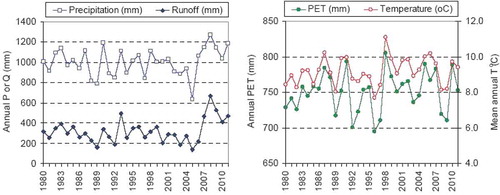
The available hydrological data include: (a) daily precipitation, P, and air temperature, T, provided by DayMet and aggregated using the USGS Geo Data Portal (Blodgett et al. 2011, Thornton et al. 2012); (b) daily potential evapotranspiration, PET, computed from temperature, using the empirical equation (2); and (c) daily discharge rate, provided by USGS and expressed in terms of equivalent depths, Q. All data series refer to a period of 32 calendar years, i.e. from 1 January 1980 to 31 December 2011. The annual urban fraction from 1980 to 2010 is also given as external information, which is extrapolated until the end of 2011. The annual values of P, T, PET and Q are plotted in Fig. 3. Interestingly, the anticipated effects of the substantially increasing urbanization cannot be recognized in the graphical representation of annual runoff (e.g. in terms of a positive trend). In fact, the signal of annual runoff generally follows the precipitation, which is reasonable since the two variables are highly correlated (r = 0.807 on an annual basis, and 0.505 on a daily basis).

Fig. 3 Plots of historical series: annual runoff and precipitation (left), and PET and temperature (right).

4 RESULTS

4.1 Evaluation of deterministic models

The first step of the proposed framework was the selection of the most suitable out of the three deterministic modelling schemes (DM0, DM1 and DM2), as explained in Section 2.7. The three models were calibrated and evaluated on the basis of both objective and subjective criteria, making use of the protocol established by Thirel et al. (2015). In general, the protocol dictated that five sub-periods are taken from the complete period, with calibration and evaluation on each of them. This is adapted to our methodology, in which, for each model, we employed the following procedure:

Initially, we attempted to calibrate the model parameters (11 for DM0 and DM1, and 16 for DM2) for the complete data period (32 years), by formulating the associated global optimization problem, adopting as objective the maximization of the model efficiency (NSE). No warming-up was accounted for, since the effect of errors in initial conditions has been practically eliminated through manual adjustment of initial storages in the three conceptual tanks. To cope with parameter uncertainty, we followed a hybrid (i.e. partially automatic and partially manual) calibration approach that aims to combine the computational power of modern optimization algorithms with the hydrological experience, thus resulting in robust and realistic parameter values (Rozos et al. 2004, Efstratiadis and Koutsoyiannis 2010, Nalbantis et al. 2011). In particular, the optimizations were carried out using the evolutionary annealing-simplex algorithm by Efstratiadis and Koutsoyiannis (2002, see also Rozos et al. 2004). For each model, we ran several optimizations of 5000 trials each, starting from different initial solution populations and also assuming different combinations of control variables as well as different parameter bounds. This approach helped to avoid local maxima and guide optimization towards solutions that are both optimal, in terms of NSE values, and consistent, in terms of hydrological behaviour. Signals of hydrological consistency were: (a) the representation of low flows; (b) the regularity of simulated state variables (snow accumulation, soil moisture storage, groundwater storage); and (c) the plausibility of optimized parameters. The reproduction of low flows was evaluated through a modified version of the NSE (NSE_LF), where the inverse transformed flows 1/(Q + ε) are used, instead of Q and ε is a small constant that allows avoidance of division by zero flows (Thirel et al. 2015). Similar to equation (17), this is defined as 1% of mean daily runoff. The regularity of the state variables was examined through graphical inspection so as to reject calibrations resulting in unreasonable long-term trends or abnormal patterns of the internal variables of the model (Efstratiadis et al. 2008, Nalbantis et al. 2011). Finally, the physical consistency of the extracted parameter values was empirically evaluated, based on our experience.

After detecting the optimal parameter values for each scheme, we calculated the nine evaluation criteria (Nash-Sutcliffe efficiency and decomposition, Nash-Sutcliffe efficiency on low flows, bias, frequency of low flows, linear correlation coefficient, relative variability in the simulated and observed discharges, bias normalized by the standard deviation of the observed discharges, modified Kling-Gupta efficiency, variation coefficient ratio) for the complete data period (1980–2011), as well as the five sub-periods, as requested by Thirel et al. (2015). The duration of each sub-period is about 2340 days or 77 months (11 688 days, in total; exact definitions of sub-periods are given in Table 1). Next, we repeated the aforementioned hybrid calibration procedure for each sub-period separately and validated for the rest of the periods/sub-periods. Hence, we extracted nine tables (i.e. one for each criterion) of size 6 × 6, where the diagonal elements indicate the criteria values in calibration and the off-diagonal ones the criteria in validation. In addition, we extracted the optimized parameter values across all periods/sub-periods. This exhaustive amount of information helped us assess the model performance stability and evaluate its predictive capacity

Table 1 NSE values across different data periods, for modelling scheme DM0. Diagonal elements indicate calibrated values, while off-diagonal elements indicate values obtained in validation (similar for Tables 2–6).

	P0	P1	P2	P3	P4	P5
Complete period P0	0.690	0.633	0.356	0.720	0.671	0.745
Sub-period P1	0.637	0.658	0.376	0.704	0.614	0.632
Sub-period P2	0.537	0.503	0.603	0.556	0.544	0.509
Sub-period P3	0.498	0.323	0.053	0.781	0.635	0.417
Sub-period P4	0.533	0.347	0.206	0.664	0.732	0.497
Sub-period P5	0.652	0.487	0.098	0.678	0.638	0.782

P0 (full period): 1/1/1980–31/12/2011; P1: 1/1/1980–31/5/1986; P2: 1/6/1986–31/10/1992; P3: 1/11/1992–31/12/1998; P4: 1/1/1999–31/8/2005; P5: 1/9/2005–31/12/2011.

Tables 1–3 show the NSE values for the three deterministic models, while Tables 4–6 give the corresponding NSE_LF values. We recall that all models were optimized against NSE, whilst NSE_LF has been used as an auxiliary criterion within the hybrid calibration procedure. As shown, DM0 and DM1 exhibit practically similar performances, both in calibration and validation. Like DM0, model DM1 has 11 parameters, and its unique difference from DM0 is the assumption of a time-varying direct runoff rate (parameter c), linearly depending on the urban area fraction (equation (12)). The introduction of this information did not improve the model uncertainty, which indicates that a more complex parameterization is required. This is offered by model DM2, which has five additional parameters for representing the surface hydrological processes. As shown in Table 3, all optimized NSE values (diagonal elements) are increased by 5–10%, while their improvement in validation (off-diagonal elements) is even higher. With respect to low flows, there is also a significant improvement of the NSE_LF scores, although the score values themselves are marginally only satisfactory. A very important advantage of model DM2 over DM0 and DM1 is its limited variability of score values across the different data periods. For instance, when DM2 is calibrated against the observed runoff of the first sub-period (P1), the NSE values across the five data periods range from 0.440 (P2) to 0.755 (P1, optimized value). In the case of models DM0 and DM1, the corresponding ranges are 0.376–0.658 and 0.341–0.658, respectively. Using the full sample of NSE scores across all different calibration and evaluation sub-periods (i.e. 5 × 5 = 25 values, in total), the corresponding coefficients of variation of NSE are 0.378 for model DM0, 0.359 for model DM1 and only 0.204 for model DM2. This indicates that model DM2 exhibits higher ‘stability’ than DM0 and DM1, since it ensures the minimum variability of NSE values (similar conclusions are drawn for the rest of the performance scores). Therefore, the model remains robust even when calibrated against a small portion of the available hydrological and urbanization information. Likewise, the 16 parameters of scheme DM2 remain quite stable, as shown in Table 7.

Table 2 NSE values across different data periods, for modelling scheme DM1.

	P0	P1	P2	P3	P4	P5
Complete period P0	0.689	0.578	0.422	0.711	0.684	0.751
Sub-period P1	0.581	0.658	0.341	0.699	0.490	0.546
Sub-period P2	0.556	0.490	0.587	0.546	0.550	0.567
Sub-period P3	0.640	0.581	0.247	0.760	0.636	0.649
Sub-period P4	0.505	0.136	0.295	0.625	0.740	0.509
Sub-period P5	0.641	0.470	0.025	0.670	0.631	0.781

Table 3 NSE values across different data periods, for modelling scheme DM2.

	P0	P1	P2	P3	P4	P5
Complete period P0	0.746	0.697	0.582	0.769	0.777	0.757
Sub-period P1	0.608	0.755	0.440	0.780	0.552	0.494
Sub-period P2	0.687	0.625	0.682	0.707	0.737	0.670
Sub-period P3	0.671	0.727	0.508	0.818	0.655	0.592
Sub-period P4	0.736	0.673	0.604	0.744	0.790	0.748
Sub-period P5	0.694	0.548	0.238	0.701	0.732	0.794

Table 4 NSE_LF values across different data periods, for modelling scheme DM0.

	P0	P1	P2	P3	P4	P5
Complete period P0	0.016	0.299	−0.028	0.050	−0.028	0.069
Sub-period P1	0.015	0.251	−0.031	0.036	−0.029	0.077
Sub-period P2	0.122	0.174	0.069	0.163	0.047	0.282
Sub-period P3	0.006	0.309	−0.035	0.058	−0.034	0.038
Sub-period P4	0.042	0.281	0.004	0.123	0.000	0.079
Sub-period P4	−0.029	−0.058	−0.068	−0.046	−0.066	0.005

Table 5 NSE_LF values across different data periods, for modelling scheme DM1.

	P0	P1	P2	P3	P4	P5
Complete period P0	−0.006	0.207	−0.047	0.028	−0.045	0.031
Sub-period P1	0.018	0.242	−0.034	0.037	−0.023	0.091
Sub-period P2	0.020	−15.480	0.025	0.139	0.014	0.195
Sub-period P3	0.027	0.366	−0.017	0.083	−0.017	0.077
Sub-period P4	−0.971	−289.764	0.042	−0.076	0.037	0.037
Sub-period P4	−0.047	−4.790	−0.070	−0.050	−0.067	0.005

Table 6 NSE_LF values across different data periods, for modelling scheme DM2.

	P0	P1	P2	P3	P4	P5
Complete period P0	0.145	0.543	0.038	0.124	0.189	0.186
Sub-period P1	0.014	0.312	−0.031	0.033	−0.011	0.035
Sub-period P2	0.210	0.633	0.392	0.169	0.076	−0.048
Sub-period P3	0.073	0.494	0.001	0.112	0.073	0.105
Sub-period P4	0.132	−11.201	0.050	0.131	0.158	0.390
Sub-period P4	0.253	−0.097	0.339	0.166	0.124	0.242

Table 7 Optimized parameter values for model DM2 across different periods.

	P0	P1	P2	P3	P4	P5
Snow processes
Degree-day factor, DDF (mm °C^‒1 d^‒1)	6.00	6.00	3.83	3.85	6.00	5.96
Max. temp. for snowfall, T0 (°C)	−1.77	0.00	−0.89	−0.65	−1.84	−3.21
Min. temp. for melting, Tm (°C)	−0.15	0.41	−0.16	−0.22	−0.09	0.06
Surface processes—Rural HRU
Direct runoff fraction, c	0.030	0.010	0.011	0.020	0.028	0.029
Soil capacity, K (mm)	573.1	557.7	392.4	587.5	483.1	433.7
Interflow threshold, H1 (mm)	499.3	506.3	336.6	530.5	430.7	225.7
Recession rate for interflow, μ (d^−1)	0.056	0.088	0.022	0.054	0.037	0.058
Recession rate for percolation, ν (d^−1)	0.001	0.002	0.002	0.002	0.001	0.001
Surface processes—Urban HRU
Direct runoff coefficient, c	0.030	0.030	0.041	0.105	0.023	0.033
Soil capacity, K (mm)	171.1	204.7	293.0	92.2	319.6	399.5
Interflow threshold, H1 (mm)	138.9	93.7	179.9	92.1	238.3	329.9
Recession rate for interflow, μ (d^−1)	0.407	0.529	0.333	0.534	0.375	0.457
Recession rate for percolation, ν (d^−1)	0.005	0.009	0.004	0.008	0.003	0.003
Groundwater processes
Baseflow threshold, Υ1 (mm)	20.1	20.6	27.4	23.6	24.3	30.0
Recession rate for baseflow, ξ (d^−1)	0.486	0.500	0.475	0.653	0.218	0.500
Recession rate for losses, φ (d^−1)	0.013	0.011	0.013	0.013	0.010	0.008

The above investigation reveals the obvious superiority of configuration DM2, based on the HRU concept, which ensures conciliation between model and parameter uncertainty. In all the following analyses, we used this scheme, with parameters optimized over the complete period (Table 7, column P0). The full range of model scores for this version of DM2 (hereafter referred to as DM2_P0) is given in Table 8, while the model fitting to the observed runoff, for the first and last sub-period of relatively low and high urbanization, respectively, are illustrated in Fig. 4.

Fig. 4 Comparison of simulated and observed runoff for sub-periods P1 (left) and P5 (right), for modelling scheme DM2_P0.

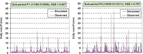
Table 8 Non-dimensional evaluation criteria for model version DM2_P0 across all periods (for their definitions, please refer to Thirel et al. 2015).

Criterion	P0	P1	P2	P3	P4	P5
NSE	0.746	0.697	0.582	0.769	0.777	0.757
NSELF	0.145	0.543	0.038	0.124	0.189	0.186
Bias (or βKGE)	0.971	0.902	1.110	0.951	1.076	0.897
FreqLF (sim.)	0.003	0.000	0.000	0.000	0.012	0.012
FreqLF (obs.)	0.021	0.000	0.044	0.002	0.038	0.018
r	0.864	0.840	0.802	0.884	0.887	0.873
aNSE	0.877	0.774	1.037	0.778	0.980	0.904
bNSE	−0.016	−0.065	0.076	−0.027	0.041	−0.054
KGE	0.831	0.765	0.764	0.779	0.837	0.836
γKGE	0.904	0.859	0.934	0.819	0.910	1.007

4.2 Investigation of model residuals and construction of stochastic error model (model EM)

In the proposed framework, the statistical behaviour of the model errors is a critical issue, and should be properly represented in the stochastic error model. Table 9 shows the statistical characteristics of the model residuals (i.e. differences between observed and simulated runoff), as well as those of the transformed residuals, which are estimated by equation (18). In contrast to the initial residuals, which are correlated with the observed runoff (r = 0.480), the transformed ones are less correlated (r = –0.235). However, the transformation through equation (18) results in a significant increase of the lag-1 autocorrelation coefficient, from ρ = 0.487 to 0.779. Moreover, the skewness coefficient is decreased, from γ = 5.595 to 1.170.

Table 9 Statistical characteristics of model residuals e_t, transformed, through equation (18), residuals w_t, and simulated errors.

	Residuals, et	Transformed residuals, wt	Synthetic errors, wt
Mean (mm)	0.026	0.099	0.099
Standard deviation (mm)	0.807	0.637	0.638
Skewness coefficient	5.595	1.170	1.178
Lag-1 autocorrelation	0.487	0.782	0.779
Cross-correlations with Q	0.480	−0.235	0.000

The elimination of the cross-correlation allows for using the simple error model (19), with φ₁ = 0.779, which reproduces the strong autocorrelation structure of the transformed errors. The radical decrease of the skewness coefficient is also very important, given that the reproduction of such high values of γ by stochastic models is practically unachievable (Koutsoyiannis 1999).

4.3 Generation of synthetic hydrological data through linear stochastic approaches (model LSM)

The next step was the generation of 1000 years of daily synthetic data for precipitation, temperature and runoff, through the three-level multivariate disaggregation scheme that has been implemented in Castalia. The generation of synthetic precipitation and temperature, the latter being used for estimating PET through equation (2), was essential for running model DM2_P0 in a stochastic simulation context. On the other hand, the generation of synthetic runoff was only made for comparison reasons, since the statistical characteristics of the historical data (i.e. the observed runoff at the basin outlet) are not representative of the future conditions of the basin, which in most studies (and herein) are handled as stationary. Stationarity is an essential hypothesis of linear stochastic models that run in steady-state simulation and are not conditioned to any ‘external’ information (in this specific case, urbanization).

The consistency of the synthetic data is evaluated by comparing the statistical properties of simulated time series against the historical ones. For convenience, evaluations are made on the grounds of the aggregated (i.e. monthly and annual) data. In particular, in Table 10 the annual mean, standard deviation, skewness coefficient and lag-1 autocorrelation for each variable are compared. The same characteristics are illustrated, by means of monthly diagrams, for the monthly time series (Figs 5–7). In Fig. 8 the monthly cross-correlations of precipitation and runoff are also plotted. As shown, the stochastic modelling scheme preserves with satisfactory accuracy all desirable statistical properties, including the major measures of variability (standard deviations and coefficients of skewness). The preservation of the statistical characteristics of historical data, which are representative of the hydrological behaviour of the real-world processes, also stands for the daily time scale. An example is given in Fig. 9, where we plot the daily time series of the three variables of interest (precipitation, runoff, PET), for the first two years of simulation. Their patterns are realistic, which indicates that the mathematical framework of Castalia, implementing linear stochastic models and simple transformations within disaggregation procedures, provides synthetic data that resemble the actual processes.

Fig. 5 Comparison of monthly statistical characteristics of observed and simulated precipitation, through the Castalia stochastic generator.

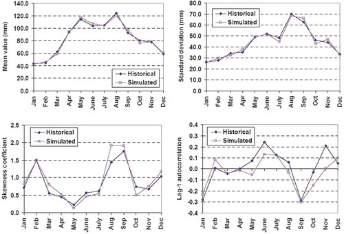
Fig. 6 Comparison of monthly statistical characteristics of observed and simulated temperature, through the Castalia stochastic generator.

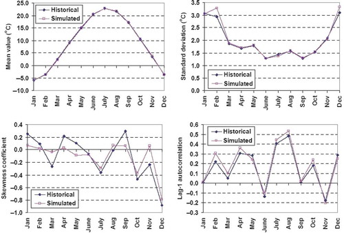
Fig. 7 Comparison of monthly statistical characteristics of observed and simulated runoff, through the Castalia stochastic generator.

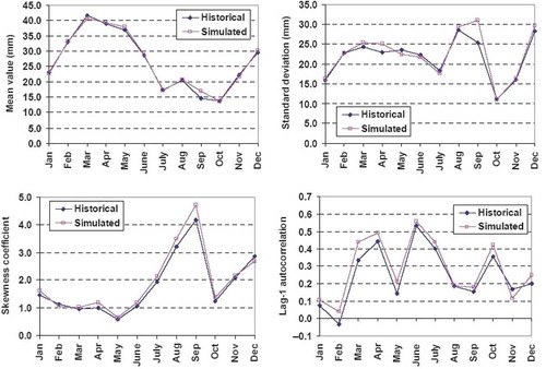
Fig. 8 Monthly and annual cross-correlations between observed precipitation (P) and runoff (Q), synthetic precipitation and synthetic runoff, generated through Castalia (model LSM), and synthetic precipitation and simulated runoff generated through model DM2_P0, for 66% urbanization fraction.

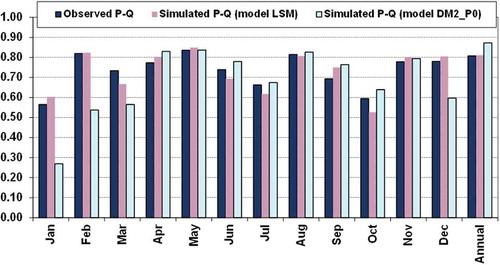
Fig. 9 Plots of daily synthetic precipitation, runoff and PET for the first two of 1000 years of simulation. Precipitation and runoff are generated through Castalia, as well as temperature data, which were then used for calculating PET.

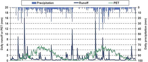
Table 10 Comparison of annual statistical characteristics for simulated variables through Castalia stochastic generator; the historical values are given in the first row while the simulated ones are found in the second row. Hurst coefficients cannot be estimated for historical samples, due to the limited length of the latter.

	Mean (mm or °C)	Standard deviation (mm or °C)	Skewness coefficient	Lag-1 auto-correlation	Hurst coeff.
Precipitation	1002.1	138.1	−0.415	0.041	–
	1004.9	137.4	−0.486	0.101	0.621
Temperature	9.17	0.77	0.206	0.173	–
	9.15	0.78	0.051	0.208	0.645
Runoff	320.1	115.5	1.038	0.398	–
	322.9	118.5	0.936	0.415	0.796

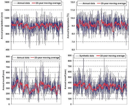
As highlighted above, although the statistical characteristics of the observed runoff are accurately reproduced in the simulated data, the latter are not usable in the context of a water planning or management study. In fact, these statistics reflect the effects of the changing (i.e. systematically increasing) urbanization during the calibration period and, therefore, may result in significant overestimation of the basin response variability with respect to a case in which the urbanization is known or fixed (e.g. because it reached saturation). In the lack of observations under steady-state conditions of the basin, the (probably) unique yet convincing evidence of this overestimation is the performance of the simulated series. As shown in Fig. 10 (lower left diagram), we detect an unrealistic (i.e. too sharp) fluctuation of runoff at the over-annual scales, which is quantified in terms of a Hurst coefficient as great as H = 0.80. The long-term persistence of runoff differs substantially from that of its driving processes, i.e. precipitation and temperature, which exhibit a reasonable scaling behaviour, as indicated by the associated Hurst coefficient values (H = 0.62 and 0.65, respectively).

Fig. 10 Plots of 1000 years of annual and 20-year moving average data for synthetic precipitation (upper left); mean temperature (upper right); synthetically generated runoff (lower left); and final runoff (lower right), generated through the combined use of deterministic and stochastic models, for the 66% urbanization scenario.

4.4 Runoff simulations using model DM2_P0 with synthetic inputs

Given that the direct stochastic approach failed to provide realistic simulations, we proceeded to use the deterministic model DM2_P0, which was fed with the already available synthetic time series of precipitation and temperature. We ran the model in steady-state mode, assuming three urban development scenarios. The first scenario refers to the current urban development, i.e. for the 1000-year simulation horizon we set a constant urban fraction of 66%. In the other two scenarios we assumed fractions of 40% and 80%, which can be considered as reasonable lower and upper limits of urban development. We note that the 40% fraction is representative of the average urban development conditions during the 32-year period of observations. These scenarios will be referred to as S66, S40 and S80 in the following.

Table 11 summarizes the statistical characteristics of the simulated runoff, which are compared with the statistics of the observed data. Comparisons are made at the annual scale, but similar conclusions stand for finer scales. By comparing the mean annual runoff values, it is shown that the river basin, even for the upper urban development scenario (S80), produces lower runoff than during the period of observations, which is not reasonable. This happens because the output of the deterministic model used for the rainfall–runoff transformation is not unbiased. In fact, there is a bias of 3% (0.026 mm d⁻¹; cf. Table 9), which is reflected in the underestimations of the mean values of the simulated runoff series. Even worse, the variability measures (standard deviation and, particularly, skewness) as well as the lag-1 autocorrelations are significantly underestimated. As discussed in the Introduction, this is a known drawback of deterministic hydrological models, i.e. the fact that they cannot explain the total variability of the observed fluxes of a river basin. However, in everyday practice, this issue is usually neglected, which leads to predictions that underrate uncertainty. On the other hand, it is important to recall once again that the statistical characteristics of the observed runoff are not fully comparable with those of the simulated runoff, due to the impacts of changing conditions during the period of observations. Thus, the variability metrics of the observed runoff should only be considered as upper limits of the associated statistics in steady-state conditions.

Table 11 Comparison of annual statistical characteristics of observed and simulated runoff. Runoff is generated by running deterministic model DM2_P0 with synthetic precipitation and temperature.

	Mean (mm)	Standard deviation (mm)	Skewness coefficient	Lag-1 auto-correlation	Hurst coeff.
Observed	320.1	115.5	1.038	0.398	–
Simulated S66	305.9	98.0	0.297	0.252	0.667
Simulated S40	286.9	92.4	0.304	0.303	0.681
Simulated S80	316.2	101.6	0.293	0.220	0.657

4.5 Runoff simulations using model DM2_P0 with synthetic inputs and considering a stochastic error term

In order to properly represent the total variability of runoff, we should account for the statistical properties of the remaining uncertainty of the deterministic model DM2_P0. In this context, the final step of the proposed framework was the introduction of a stochastic error term to the simulated runoff, thus providing fully consistent synthetic runoff data. This step was not straightforward and required an iterative procedure, as follows:

First, we produced 1000 years of synthetic w_t (~365 250 values, in total), employing equation (19), in which the random variables z_t were produced by a three-parametric gamma generator. By examining the statistical characteristics of the simulated w_t for different simulation lengths we found that the 1000 years were absolutely necessary for reproducing the theoretical statistics of Table 9 (particularly, the coefficient of skewness, γ = 1.170) with high accuracy. The w_t values were next transformed back to error terms, e_t, by considering the synthetic runoff values, Q_sim,t, obtained through the combined use of models LSM and DM2_P0, and then applying equation (23).

However, due to the nonlinearity of equations (23) and (24), the preservation of the statistical characteristics of the parent residual terms, which are shown in Table 9, is not guaranteed, although the statistics of the simulated w_t values are explicitly preserved in the theoretical model (Table 9). This approach was repeated for the three sets of simulated runoff, which refer to the three urban development scenarios.

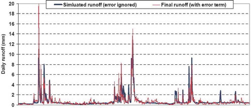
After obtaining a sequence of e_t value, we added them to the corresponding Q_sim,t, to obtain the final data of synthetic runoff. An example of the difference between the daily runoff series, considering the error term or not, is illustrated in Fig. 11. As shown, during the low flow periods the introduction of the error term results in slight fluctuations. Conversely, the daily peaks may change considerably, as expected, due to heteroscedasticity. Actually, the uncertainty of any deterministic hydrological model in the region of high flows is much higher than in the case of normal and low flows, and this uncertainty should also be reflected in the simulated data.

Fig. 11 Comparison of daily synthetic runoff data for the first two years of simulation obtained through model DM2_P0 fed with synthetic inputs, by considering or not the error term. Simulations refer to the 66% urbanization scenario.

Table 12 gives the statistical characteristics of the final runoff data, which are contrasted to the statistics of the observed runoff. By considering the error term, the mean values for all urban development scenarios are increased with respect to the values given in Table 11 and, similarly, the variability metrics (standard deviation and skewness) are increased, as required. However, the lag-1 autocorrelations and the Hurst coefficients are not affected by adding up the error term, which is strongly desirable. Similar conclusions arise for the monthly time scale, for which we provide detailed statistical comparisons for the three scenarios, in Figs 12–14.

Fig. 12 Comparison of monthly statistical characteristics of simulated runoff, with and without considering the error term, assuming 40% urbanization fraction.

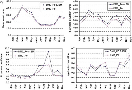
Fig. 13 Comparison of monthly statistical characteristics of simulated runoff, with and without considering the error term, assuming 66% urbanization fraction.

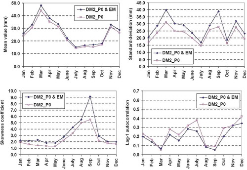
Fig. 14 Comparison of monthly statistical characteristics of simulated runoff, with and without considering the error term, assuming 80% urbanization fraction.

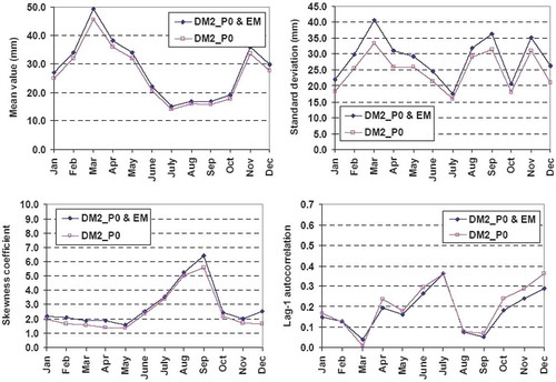
Table 12 Comparison of annual statistical characteristics of observed and simulated runoff. Runoff is generated by running deterministic model DM2_P0 with synthetic precipitation and temperature, and then adding a stochastic error term.

	Mean (mm)	Standard deviation (mm)	Skewness coefficient	Lag-1 auto-correlation	Hurst coeff.
Observed	320.1	115.5	1.038	0.398	–
Simulated S66	328.8	115.2	0.567	0.242	0.664
Simulated S40	307.5	106.2	0.461	0.246	0.672
Simulated S80	338.6	114.9	0.446	0.167	0.629

Following the proposed framework, we anticipate that the final synthetic data do ensure both physical and statistical consistency. As explained above, this consistency cannot be strictly evaluated, due to the temporally-varying conditions in the study catchment during the period of observations. It is important to note that the effects of urbanization on runoff generation are not so impressive. The mean annual runoff under steady-state conditions, as estimated through stochastic simulation, increases by only 10% (i.e. from 307.5 to 338.6 mm) for an increase of urbanization fraction from 40% to 80%. This conclusion is in line with the historical data, given that no remarkable trend of runoff has been indicated during three decades of substantial increase of urbanized areas. Apparently, in the specific catchment, urbanization refers to a rather mild development (e.g. residential areas), which does not significantly change the average response of the basin. Anyway, the limited impacts of urbanization, at least at the mean annual scale, should not be surprising, since similar conclusions have been extracted in several modelling studies worldwide (e.g. Du et al. 2012).

5 CONCLUSIONS AND DISCUSSION

The research results presented in this paper mainly address five research questions (see Section 2.1) dealing with hydrological modelling of catchments with temporally-varying characteristics. The focus was on systematic changes in catchment properties, and we used urbanization as our working example of such changes. A number of conclusions are drawn, listed below, in line with the five questions originally posed.

1. A modelling framework was set up by combining stochastic and deterministic models in an attempt to exploit the advantages of the two approaches. Our ultimate goal was to provide synthetically generated runoff predictions with consistent statistical characteristics for use in water resources studies. The proposed modelling framework involved two phases: (a) calibrating a deterministic hydrological model through a hybrid (manual/automatic) procedure, which exploits the capability of the parameter estimation protocol by Thirel et al. (2015) (a stochastic model for model errors was also calibrated in this phase); and (b) using a linear stochastic model to generate inputs fed to the deterministic model that yields simulated responses of the basin under study; errors are added to these responses, which are synthetically generated via the error model.

2. An essential part of the proposed modelling framework is the use of a deterministic hydrological model; in our work this was effectively parameterized to account for the kind of change selected (i.e. growing urbanization). Two parameterizations were tested: a lumped model with 11 parameters, one of which is related to the known urban area fraction, and a 16-parameter model which involves two hydrological response units (HRUs), representing urban and rural areas of time-varying surface area. In our tests, we found no essential increase in performance of the lumped model over its counterpart without consideration of urbanization. Contrary to this, the HRU-based approach allowed a gain in NSE of 5–10%; the gain in terms of low-flow efficiency was even higher. Through calibration on part of the available data, we obtained a model that is robust in terms of performance and parameter values.

3. The final parameterization of the deterministic model resulted as a compromise between model and parameter uncertainty, i.e. the minimum required parameterization that allows an acceptable model performance where the latter is dictated by experience. Passing from an 11-parameter model to a 16-parameter one was judged to be necessary. The protocol of Thirel et al. (2015) was critical for enhancing model robustness within a frame of hybrid calibration.

4. It was shown that a linear stochastic approach can result in unrealistic variability of the basin responses, which is reflected in a large discrepancy between the Hurst coefficient of inputs (around 0.65) and the response (0.80); conversely, our nonlinear stochastic modelling framework brings the variability of these responses down to a value that is justified by the variability of the input. This indicated a higher credibility over the linear stochastic approach.

5. With regard to the known drawback of deterministic hydrological models, i.e. the fact that these underrate the total variability of the observed responses of a river basin, our research results confirmed that using an appropriate error model can tackle the problem effectively. The best deterministic model resulted in a bias in the mean runoff of 3%, while higher downward bias appeared in the variability measures (standard deviation and skewness) as well as the lag-1 autocorrelations. In our case a stochastic error model of the autoregressive family was designed, based on log-transformed residuals.

The testing experiment also revealed the benefits of information across all steps of the modelling procedure. Obviously, the observed hydrological data were an essential yet not unique component of this information. The hydrological experience also played a key role, since the evaluation of models was also based on subjective criteria and empirical judgment. By this it is meant that we exploited knowledge of the model structure in a series of successive sessions of parameter optimization, with manual adjustment of the parameter space boundary between these sessions. We also highlighted that the available information of urbanization growth allowed the formulation of a nonlinear stochastic model for representing the runoff. In the absence of such information, the use of a linear stochastic model, considering the statistical characteristics of the observed runoff, would be mandatory. However, the apparent lack of information about the future conditions of the basin was handled by running steady-state scenarios of time-invariant urban development. Under this premise, probable future changes of the basin mechanisms are effectively represented by stochastic approaches hypothesizing stationarity.

In closing, we wish to reiterate the fact that the hydrological models used in this work are viewed as tools or methods that assist in a wide spectrum of applications in water resources management, where decisions are taken under high uncertainty. One form of such uncertainty is due to the kind of change that we treated in this study, i.e. growing urbanization. The results of this work let us believe that the proposed framework can be an effective way to account for any systematic changes in water resources systems. We also note that the choice of the simulation setting also depends on the extent of such changes. For instance, it appears that, in the studied catchment, urbanization is related to mild changes in land cover, which are not reflected in pronounced changes in the average response of the basin. Therefore, even a linear stochastic model in a stationary setting would provide quite realistic results, although with overestimated variability. In any case, since the actual variability of the basin’s responses is impossible to know, catchment models should definitely handle these responses as stochastic processes.

Disclosure statement

No potential conflict of interest was reported by the author(s).

Acknowledgements

We wish to thank Guillaume Thirel and Vazken Andréassian for their kind invitation to submit our work to this special issue. We also wish to thank the two anonymous reviewers, as well as the Guest Editor, Dr Thirel, for their constructive comments and suggestions.

REFERENCES

- Andréassian, V., et al., 2009. HESS Opinions “Crash tests for a standardized evaluation of hydrological models”. Hydrology and Earth System Sciences, 13, 1757–1764. doi:10.5194/hess-13-1757-2009
- Andréassian, V., et al., 2010. Editorial—The Court of Miracles of Hydrology: can failure stories contribute to hydrological science? Hydrological Sciences Journal, 55 (6), 849–856. doi:10.1080/02626667.2010.506050
- Blazkova, S. and Beven, K.J., 2004. Flood frequency estimation by continuous simulation of subcatchment rainfalls and discharges with the aim of improving dam safety assessment in a large basin in the Czech Republic. Journal of Hydrology, 292, 153–172. doi:10.1016/j.jhydrol.2003.12.025
- Blodgett, D.L., et al., 2011, Description and testing of the Geo Data Portal: Data integration framework and Web processing services for environmental science collaboration. US Geological Survey Open-File Report 2011–1157, 9, available only at http://pubs.usgs.gov/of/2011/1157/
- CMAP (Chicago Metropolitan Agency for Planning), 2011. Ferson-Otter Creek Watershed Plan available at: http://foxriverecosystem.org/ferson_otter.htm
- Du, J., et al., 2012. Assessing the effects of urbanization on annual runoff and flood events using an integrated hydrological modeling system for Qinhuai River basin, China. Journal of Hydrology, 464–465, 127–139. doi:10.1016/j.jhydrol.2012.06.057
- Efstratiadis, A. and Koutsoyiannis, D., 2002. An evolutionary annealing-simplex algorithm for global optimisation of water resource systems. Proceedings of the Fifth International Conference on Hydroinformatics. Cardiff: International Water Association, 1423–1428.
- Efstratiadis, A., et al., 2008. HYDROGEIOS: a semi-distributed GIS-based hydrological model for modified river basins. Hydrology and Earth System Sciences, 12, 989–1006. doi:10.5194/hess-12-989-2008
- Efstratiadis, A. and Koutsoyiannis, D., 2010. One decade of multi-objective calibration approaches in hydrological modelling: a review. Hydrological Sciences Journal, 55 (1), 58–78. doi:10.1080/02626660903526292
- Efstratiadis, A., 2011. New insights on model evaluation inspired by the stochastic simulation paradigm. European Geosciences Union General Assembly 2011, Vienna. Geophysical Research Abstracts, 13, 1852. European Geosciences Union. Available at: http://itia.ntua.gr/1116/
- Efstratiadis, A., et al., 2014. A multivariate stochastic model for the generation of synthetic time series at multiple time scales reproducing long-term persistence. Environmental Modelling and Software, 62, 139–152. doi:10.1016/j.envsoft.2014.08.017
- Fiorentino, M., Salvatore, M., and Iacobellis, V., 2007. Peak runoff contributing area as hydrological signature of the probability distribution of floods. Advances in Water Resources, 30, 2123–2144. doi:10.1016/j.advwatres.2006.11.017
- Flügel, W.-A., 1995. Delineating hydrological response units by geographical information system analyses for regional hydrological modelling using PRMS/MMS in the drainage basin of the River Bröl, Germany. Hydrological Processes, 9, 423–436. doi:10.1002/hyp.3360090313
- Franchini, M., Hashemi, A.M., and O’Connell, P.E., 2000. Climatic and basin factors affecting the flood frequency curve: Part II—a full sensitivity analysis based on the continuous simulation approach combined with a factorial experimental design. Hydrology and Earth System Sciences, 4, 483–498. doi:10.5194/hess-4-483-2000
- Gelfan, A.N., 2010. Extreme snowmelt floods: frequency assessment and analysis of genesis on the basis of the dynamic-stochastic approach. Journal of Hydrology, 388, 85–99. doi:10.1016/j.jhydrol.2010.04.031
- Hrachowitz, M., et al., 2013. A decade of predictions in ungauged basins (PUB)—a review. Hydrological Sciences Journal, 58 (6), 1198–1255. doi:10.1080/02626667.2013.803183
- Katz, R.W. and Parlange, M.B., 1998. Overdispersion phenomenon in stochastic modeling of precipitation. Journal of Climate, 11, 591–601. doi:10.1175/1520-0442(1998)011<0591:OPISMO>2.0.CO;2
- Koutsoyiannis, D., 1999. Optimal decomposition of covariance matrices for multivariate stochastic models in hydrology. Water Resources Research, 35 (4), 1219–1229. doi:10.1029/1998WR900093
- Koutsoyiannis, D., 2000. A generalized mathematical framework for stochastic simulation and forecast of hydrologic time series. Water Resources Research, 36 (6), 1519–1533. doi:10.1029/2000WR900044
- Koutsoyiannis, D., 2001. Coupling stochastic models of different time scales. Water Resources Research, 37 (2), 379–391. doi:10.1029/2000WR900200
- Koutsoyiannis, D., 2011. Hurst-Kolmogorov dynamics and uncertainty. Journal of the American Water Resources Association, 47 (3), 481–495, doi:10.1111/j.1752-1688.2011.00543.x
- Koutsoyiannis, D., 2013. Hydrology and change. Hydrological Sciences Journal, 58 (6), 1177–1197. doi:10.1080/02626667.2013.804626
- Koutsoyiannis, D., 2014. Entropy: from thermodynamics to hydrology. Entropy, 16 (3), 1287–1314. doi:10.3390/e16031287
- Koutsoyiannis, D., Onof, C., and Wheater, H.S., 2003. Multivariate rainfall disaggregation at a fine time scale. Water Resources Research, 39 (7), 1173. doi:10.1029/2002WR001600
- Kuchment, L.S. and Gelfan, A.N., 2002. Estimation of extreme flood characteristics using physically based models of runoff generation and stochastic meteorological inputs. Water International, 27, 77–86. doi:10.1080/02508060208686980
- Kuczera, G., et al., 2010. There are no hydrological monsters, just models and observations with large uncertainties! Hydrological Sciences Journal, 55 (6), 980–991. doi:10.1080/02626667.2010.504677
- Matalas, N.C. and Wallis, J.R., 1976. Generation of synthetic flow sequences. In: A.K. Biswas, eds. Systems approach to water management. New York: McGraw-Hill.
- Montanari, A. and Koutsoyiannis, D., 2012. A blueprint for process-based modeling of uncertain hydrological systems. Water Resources Research, 48, W09555. doi:10.1029/2011WR011412
- Montanari, A., et al., 2013. “Panta Rhei”—everything flows: change in hydrology and society—the IAHS scientific decade 2013–2022. Hydrological Sciences Journal, 58 (6), 1256–1275. doi:10.1080/02626667.2013.809088
- Nalbantis, I., 2000. Real-time flood forecasting with the use of inadequate data. Hydrological Sciences Journal, 45 (2), 269–284. doi:10.1080/02626660009492324
- Nalbantis, I., et al., 2011. Holistic versus monomeric strategies for hydrological modelling of human-modified hydrosystems. Hydrology and Earth System Sciences, 15, 743–758. doi:10.5194/hess-15-743-2011
- Nalbantis, I., Obled, C., and Rodriguez, J.Y., 1995. Unit hydrograph and effective precipitation identification. Journal of Hydrology, 168, 127–157. doi:10.1016/0022-1694(94)02625-L
- Oudin, L., et al., 2005. Which potential evapotranspiration input for a lumped rainfall–runoff model? Part 2—towards a simple and efficient potential evapotranspiration model for rainfall–runoff modelling. Journal of Hydrology, 303 (1–4), 290–306. doi:10.1016/j.jhydrol.2004.08.026
- Rozos, E., et al., 2004. Calibration of a semi-distributed model for conjunctive simulation of surface and groundwater flows. Hydrological Sciences Journal, 49 (5), 819–842. doi:10.1623/hysj.49.5.819.55130
- Sikorska, A., Montanari, A., and Koutsoyiannis, D., 2014. Estimating the uncertainty of hydrological predictions through data-driven resampling techniques. Journal of Hydrologic Engineering (ASCE), A4014009. doi:10.1061/(ASCE)HE.1943-5584.0000926
- Sorooshian, S. and Dracup, J.A., 1980. Stochastic parameter estimation procedures for hydrologic rainfall–runoff models: correlated and heteroscedastic error cases. Water Resources Research, 16 (2), 430–442. doi:10.1029/WR016i002p00430
- Suweis, S., et al., 2010. Impact of stochastic fluctuations in storage-discharge relations on streamflow distributions. Water Resources Research, 46 (3), W03517. doi:10.1029/2009WR008038
- Thirel, G., et al., 2015. Hydrology under change: an evaluation protocol to investigate how hydrological models deal with changing catchments. Hydrological Sciences Journal, 60 (7-8). doi:10.1080/02626667.2014.967248
- Thornton, P.E., et al., 2012. Daymet: Daily surface weather on a 1 km grid for North America, 1980–2011. Acquired online (http://daymet.ornl.gov/) on 23/12/2012 from Oak Ridge National Laboratory Distributed Active Archive Center, Oak Ridge, Tennessee, USA. doi:10.3334/ORNLDAAC/Daymet_V2