Simulating streamflow variability and aquatic states in temporary streams using a coupled groundwater-surface water model

Abstract

In order to apply the EU Water Framework Directive for temporary streams, it is important to quantify the space–time development of different aquatic states. We report on research on the development of aquatic states for temporary streams in the Evrotas basin, Greece. The SIMGRO regional hydrological model was used in a GIS framework to generate flow time series for the Evrotas River and all major tributaries. Five flow phases were distinguished: flood conditions, riffles, connected pools, isolated pools and dry bed conditions. Thresholds based on local hydraulic characteristics were identified per stream reach and flow phase, enabling the frequency of flow phases per month and the average frequencies for all streams to be derived. Three historical scenarios within the 20th century, marking periods of major changes in water management, were investigated. Additionally, a climate scenario for the 2050s was analysed. Simulations revealed that low flows are now much lower, mainly because more groundwater is abstracted for irrigation. The consequence is that stretches of the river fall dry during several months, causing the ecological status to deteriorate.

Editor Z.W. Kundzewicz Associate editor X. Chen

Key words:

• aquatic community
• temporary streams
• flow phases
• pools
• river basin
• SIMGRO model
• Greece

1 Introduction

Regions with water stress are a recurring and worldwide phenomenon and their spatial and temporal characteristics vary significantly because of hydro-climatic and river basin conditions. In the countries around the Mediterranean Sea, for example, summers are generally long and dry, and therefore the water resources are intensively exploited during this season. This results in water scarcity, distinct seasonal dry periods and often a non-permanent flow regime (Grindlay et al. 2011). For the main streams in the river basin, the flow regime is temporary. The smaller streams found in the headwaters are generally ephemeral streams; these flow during, and immediately after a precipitation event, meaning a flow exists for a short period. Temporary streams have a non-permanent or intermittent flow regime, usually falling dry for a distinct seasonal period (Uys and O’Keeffe 1997, Moraetis et al. 2010). Therefore, we use the term ‘temporary streams’ in this paper for the major streams in the Mediterranean region.

Despite their importance (Lake 2003, Boulton 2003), temporary streams have received little attention from the hydrological research community. Their hydrological processes and water quality dynamics are still incompletely understood, and therefore there is inadequate basis for developing water management strategies. The duration of dry periods is often extended by the abstractions of surface water and groundwater for drinking water, industry or agriculture. Temporary streams often result in bad water quality and their disconnected reaches are even more critical in terms of their ecological status. The water quantity has great impact on the ecological status of temporary rivers, as it affects the survival of aquatic species and their ability to recolonize tributaries or stretches (Skoulikidis et al. 2011). The ecological status depends on whether the riverbed dries out completely during periods of no flow or whether pools remain, and also on the duration and frequency of these dry spells, which may change from year to year (Munné and Prat 2011).

The Water Framework Directive (WFD) is an initiative aimed at improving water quality throughout the European Union. Although the WFD does not use the term environmental flow explicitly, it requires member states to achieve good ecological status in all water bodies. Temporary streams are not specifically addressed (Acreman and Ferguson 2010, Vardakas et al. 2010). At this stage the implementation, of the WFD and the development of river basin management plans is inadequate for temporary streams and urgently requires new concepts of hydrological and ecological characterization.

Classical methods of assessing streamflow characteristics such as those based on mean monthly discharge have only very limited value for assessing the impact of pressures and measures on ecologically sensitive water bodies for planning effective watershed management. In some areas of Europe, such as the Mediterranean region, where there are many streams, there is a dearth of basic spatial and temporal information on the available volume of water (e.g. Bull and Kirkby 2002). An added complication is that the intermittence of many streams is expected to increase in the future in response to anthropogenic pressure and climate change (Larned et al. 2010). These remarks underline the need to understand and manage the consequences of adverse ecological effects (Boulton 2003).

Generally, hydrological models are classified according to the hydrological subsystem they consider: saturated groundwater models, unsaturated zone models and surface water models. Advances in computer technology and the reduction in computational time have made it possible to integrate the subsystems into hydrological response models. The pioneering work done by Freeze (Freeze and Harlan 1969) on integrated modelling in a physically-based approach deserves to be mentioned. Some models consider the integration of groundwater (saturated and unsaturated zones) and surface water. The SWAT model (Arnold et al. 1998) is developed to predict the impact of land management practices on water, nutrients, sediments and agricultural yields in large complex watersheds with varying soils, land-use and management conditions over long periods of time. In addition, model applications involved the coupling with MODFLOW to simulate the regional groundwater flow (Chen et al. 2007). The hydrological model MIKE SHE (Abbott et al. 1986) has been developed to provide solutions in water resources studies, where problems arising from conjunctive use of water need to be solved. The MIKE SHE model is a physically-based distributed catchment modelling system. The distributed, physically-based CATHY model (Camporese et al. 2010) integrates land surface and subsurface flow processes. The three-dimensional Richards equation is used for variably saturated flow in porous media, whereas a path-based one-dimensional diffusion wave equation is used for hill slope and stream channel flow. The InHM model (Ebel et al. 2009) integrates surface and subsurface flows and transport processes in one framework. The ParFlow model (Kollet and Maxwell 2006) is an open-source watershed flow model. It includes a fully integrated overland flow module, the ability to simulate complex topography, geology and heterogeneity, and coupled land-surface processes. The SIMPRO model (Querner 1986) was a first attempt to link a surface water model with a relatively simple one-dimensional model of both the saturated and unsaturated zones. Regional groundwater flow was not considered in the model. To include regional groundwater flow a simple approach was adopted for the surface water in the regional hydrological model SIMGRO (Querner 1997). The interaction between groundwater and surface water in the model follows the classical approach reported by Ernst (1978) using a head difference and a drainage resistance.

The research carried out in the EC-funded MIRAGE project (Froebrich et al. 2010) resulted in a framework for managing the Mediterranean water bodies dominated by temporary streams. A method has been developed to characterize the actual spatio-temporal distribution of streamflow under different aquatic states at the sub-basin scale (Gallart et al. 2012). The concept of aquatic states is related to flow phases and the development and abundance of the different mesohabitats that determine the structure and composition of the aquatic assemblages (riffles and pools and the existence of connections between them). The classification method is based on flow frequency analysis and uses field observations and discharge measurements. This information is available for points (i.e. gauging stations), and so is often insufficient to describe the actual water availability and ecological status across sub-basins in dry periods. We therefore have used a hydrological model to support the determination of the hydrological constraints to aquatic biota and thus the determination of the ecological status of temporary streams. Our aim was to be able to distinguish the discontinuities between different aquatic states, as these are crucial for the development of aquatic biota (Boulton 2003). In this paper, as well as using observed time series, we applied the SIMGRO regional hydrological model to generate the necessary river flow data to be analysed in terms of ecological status. SIMGRO is incorporated in a GIS, which makes it easier to relate the spatial-temporal characteristics of the different types of aquatic states and to link these to catchment characteristics. We applied the model to the Evrotas basin in Greece, to demonstrate the viability of the method and to investigate the mechanisms underlying it. Some reasons for selecting the Evrotas River basin were the availability of ecological field data and because water resources are under pressure due to the increase in agriculture and irrigation over the past 50 years.

2 Flow characterization and classification

Several classifications of the degree of non-permanence of streams have been developed in the past in order to assess hydrological regimes. Two classifications deserve mentioning. Poff (1996) defined three major classes of non-permanent flow: the harsh intermittent class is more than 90 days per year with no flow; intermittent flashy or intermittent runoff is when more than 10 days per year have no flow; and permanent streams are those with less than 10 days per year with no flow. The flow regime classification devised by Kennard et al. (2010) is more specific. There are 12 classes. Classes 1 to 4 are streams of varying degrees of permanence and classes 5 to 12 are temporary streams. The temporary streams are subdivided into streams that rarely cease to flow, regularly stop flowing and are extremely intermittent. However, the existing classifications rarely consider ecological effects and instead are based on hydrology (Gallart et al. 2012). The factors critical for aquatic life are the duration of the no-discharge period and the presence, size, permanence and physicochemical conditions of individual residual pools. Bonada et al. (2007) proposed a typology of streams based on aquatic communities that are most sensitive to the availability of residual water during the dry season: permanent (P); intermittent-pools (IP); intermittent-dry (ID) and episodic-ephemeral (E). If pools persist, many species can colonise the stream and, at this point, the species richness may be similar to, or higher than in permanent streams (Bonada et al. 2007). If the pools are small and not replenished with water from the underlying alluvium, the pool starts to dry up as the water evaporates, and the fauna are trapped in a shrinking volume of water whose physicochemical characteristics are degrading rapidly. In such extreme conditions, only a few species are able to survive (Lake 2003). At the end of the dry period in summer, the streambed commonly contains a mosaic of pools in different states: large pools of good water quality, containing fish, may coexist with small, highly polluted pools that are devoid of macro fauna. This spatial diversity in pool size and condition throughout a catchment must be adequately described in order to understand the river basin’s ecological status and to implement appropriate management. For instance, water abstraction results in enormous changes not only in the duration of flow periods but also in the number and condition of pools (Datry et al. 2011).

Based on the work of Bonada et al. (2007), Gallart et al. (2012) proposed a classification of the hydrological conditions of temporary rivers based on field observations and discharge measurements that is relevant for ecology. The six aquatic states from the point of view of the aquatic organism are: hyperheic (flood conditions); eurheic (riffles dominant with pools present); oligorheic (scarce riffle areas connecting pools); arheic (isolated pools) and hyporheic or edaphic (dry bed conditions) and shown in Table 1. They describe the range of flow stages from high water levels not exceeding the bank-full situation, to the dry stage with zero flow, and relate them to the existence and relative abundance of the two main mesohabitats present in the temporary streams (pools and riffles) and their interconnectedness. We applied this classification to the flow situations generated by the hydrological model, where specific thresholds separate the different statuses.

Table 1. Basic flow characterization thresholds adopted for classifying the model results for the Evrotas basin (adapted from Gallart et al. 2012).

Aquatic states	Flow phases	Description
Hyperheic	Flood	High flow stages exceeding bank-full and with generalized transport of bed sediment
Eurheic	Riffles	Gradient and morphology give abundant riffles (visible continuous surface flow)
Oligorheic	Connected pools	Abundant pools generally connected by water rivulets
Arheic	Pools	Abundant pools, no flow between them
Hyporheic	Dry stream	Channel is dry but alluvium is wet
Edaphic	Dry alluvium	Channel and alluvium are dry

The flow regime of each stream reach differs, depending on factors like stream width, bed slope, channel roughness and morphology. Therefore, the thresholds between the flow phases should also consider these local aspects. In our research we used hydraulic criteria: the water depth, and the width and bed slope of a stream. The derived thresholds and the flow frequency curve of a stream are used to create an aquatic states frequency graph (ASFG) (see Gallart et al. 2012). Such a graph describes the mean annual prevalence and timing of aquatic states for a stream reach. An example is presented below.

Two factors are important for the viability of an aquatic ecosystem in a temporary river: how long the river falls dry each year and whether the occurrence is seasonal (Lytle and Poff 2004, Datry et al. 2011). These data can be used to estimate the potential for a viable aquatic community (Gallart et al. 2008). If a river falls dry regularly, the aquatic community will adapt and therefore increase its chances of surviving a dry spell (Magalhães et al. 2007). The longer the dry period, the fewer species can survive, and only the resilient ones that have adapted to the circumstances will remain (Lake 2003).

In the Mediterranean region in spring, the flow conditions are very important for the river ecosystem because most aquatic and amphibian species reproduce in this season. If the river is dry for a long time during this period, populations of these species will suffer (Gasith and Resh 1999). It is therefore important that in spring (mid-March until mid-June) a river reach contains flowing water and the aquatic states range from connected pools to flood. This will enable most species to reproduce successfully and allow the development of a community of macro-invertebrates similar to that found in permanent streams (Bonada et al. 2007). This is particularly true for streams whose dry period is recurrent (e.g. the Mediterranean area), in contrast to streams in areas where the drought is not so predictable, as in some parts of Australia (Boulton 2003). Therefore in summary, temporary streams must meet three criteria in order to support a community similar to (or even more diverse than) that found in permanent streams:

1. In spring, the flow must last for more than two months. In the modelling analysis we assumed spring was from March to June.

2. The streambed should not fall fully dry for more than 3 months in total per year.

3. If flow ceases for more than 3 months, residual pools of sufficient water quality must be present throughout that period.

3 Description of the SIMGRO model

The SIMGRO (SIMulation of GROundwater and surface water levels) model is a distributed parameter model that simulates regional transient saturated groundwater flow, unsaturated flow, actual evapotranspiration, sprinkler irrigation, streamflow, groundwater and surface water levels as a response to rainfall, reference evapotranspiration and groundwater abstraction (Fig. 1). The integration of groundwater and surface water in the model enables water to be stored as groundwater or as surface water. This is crucial in order to simulate the behaviour of the river flow response satisfactorily. For a comprehensive description of SIMGRO, including all model parameters and validation, see Querner (1997). Practical applications of the model use have been described elsewhere, for river basins (Querner and Povilaitis 2009) and for hydrological drought analysis (Querner and Van Lanen 2010).

Figure 1. Schematization of water flows in the SIMGRO model. The main feature of this model is the integration of saturated and unsaturated zones and the surface water systems within a sub-catchment (Querner 1997).

To model the hydrology of a region, the system has to be schematized geographically, both horizontally and vertically. The horizontal schematization allows different land uses and soils to be input per node, to make it possible to model spatial differences in evapotranspiration and moisture content in the unsaturated zone. Vertically, two reservoirs, one for the root zone and one for the underlying soil (Fig. 1), represent the unsaturated zone. Evapotranspiration is a function of the crop and the moisture content in the root zone. To calculate the actual evapotranspiration, it is necessary to input the measured values for net precipitation, and the potential evapotranspiration for a reference crop (grass) and woodland. The model derives the potential value for other crops or vegetation types from the values for the reference crop, by converting with known crop factors (Allen et al. 1998). In the SIMGRO model, the irrigation gifts can be assigned automatically, based on the moisture content in the root zone (automatic). Each crop can be assigned a particular threshold value at which irrigation should start. This method is used in situations where farmers use sprinkler irrigation and individually abstract the water from surface water and/or groundwater (Querner et al. 2008).

In SIMGRO, the finite element procedure is applied to represent the flow equation that describes transient groundwater flow in the saturated zone. Various aquifers and aquitards can be considered and SIMGRO permits spatially-distributed parameters to be specified. A transmissivity is allocated to each node to account for the regional hydrogeology. A number of nodes make up a sub-catchment to be considered for the surface water in the model.

The rather complex process of surface runoff is simplified in the SIMGRO model by a reservoir (depression storage). The precipitation is stored in this reservoir with the infiltration occurring at the bottom. The infiltration rate has an upper limit. When the depression reservoir is full, the excess is treated as surface runoff (Querner 1997).

In the model, the surface water system is considered as a network of reservoirs. The inflow of one reservoir may be the discharge of the various streams, ditches and surface runoff. The outflow from one reservoir is the inflow to the next downstream reservoir. The stage depends on surface water storage and on reservoir inflow and discharge. In the model, three types of drainage subsystem are used to simulate the aquifer–surface water interaction and classified to their size. The three subsystems are ditches, tertiary water courses and the major streams. This interaction is simulated for each drainage subsystem using a drainage resistance and the difference in level between groundwater and surface water (Ernst 1978). Details on the use of the drainage resistance concept and parameters are given in Querner (1997). The parameters for the drainage subsystems may vary over the modelled area. Furthermore, snow accumulation and melting has been accounted for in the model, based on the daily average temperature.

The model was used within the GIS environment ArcView. The AlterrAqua (Povilaitis and Querner 2006) user interface served to convert digital geographical information (soil map, land use, watercourses, etc.) into input data for the model. Model results can be visualized and analysed together with specific input parameters. For the flow characterization, calculated discharges were analysed in terms of flow exceedence. Using hydraulic characteristics for each individual stream gives the thresholds (see Section 4.2 on discharge thresholds between aquatic states). The calculated discharges and the derived thresholds were used to estimate the frequency of the flow phases (Table 1) for each month.

4 Modelling the Evrotas basin and scenario analysis

4.1 Study area and model schematization

The Evrotas River basin is situated in the southern Peloponnese, Greece (Fig. 2), and has an area of 2410 km². The main river is about 90 km long (Gamvroudis et al. 2011) and flows south into the Laconian Gulf of the Mediterranean Sea. The Evrotas basin is bordered in the east and west by mountain ridges up to 2400 m a.s.l. The valley bottom is filled with fluvial sediments. Karstic aquifers are responsible for the numerous springs that discharge water into the Evrotas River. The predominant land use is agriculture, mainly olive groves and orange orchards. Only 1% of the area is built up. The remaining area is under natural vegetation (Tzoraki et al. 2011, 2013). The mean annual precipitation during 2000–2008 was 803 mm (Vardakas et al. 2010). Most precipitation occurs during autumn and winter. The summers are dry, with about 5–10% of the yearly rainfall.

Figure 2. The major streams in the Evrotas River basin, Greece.

The mean annual discharge of the Evrotas is 3.3 m³ s^-1 (1974–2008) as measured at the gauge near Vrontamas (for location see Fig. 2). During the 1970s, the average discharge was around 4.9 m³ s^-1 and at present it is 2.0 m³ s^-1 (Skoulikidis et al. 2010). Stretches of the Evrotas now fall dry during several months each year. The tributaries are commonly temporary streams. In recent decades the irrigated area has greatly increased. The irrigation water was originally from surface water; since the 1960s groundwater is also used. In the Evrotas basin there are now more than 3700 wells used by the public and private sectors to extract water for irrigation, industry and domestic consumption. The increased exploitation of the groundwater resources has caused the water table to fall dramatically.

In order to schematize the groundwater system in the Evrotas basin we used a finite element network with 13 424 nodes spaced about 500 m apart. We divided the model area into 544 sub-basins, using the river and its main tributaries for the flow routing. Dominant soil and rock types are alluvium, limestone and schist. Very little is known about the subsurface of the Evrotas basin. For example, no information on pumping tests was available to assess the conductivity. There is also uncertainty about the occurrence and thickness of the layers in the model. However, using geological maps it was possible to deduct some additional information on the geology of the area. For the groundwater system we considered three layers, two aquifers separated by an aquitard, ranging from 50–100 m thickness. The transmissivity of the two aquifers was based on the geological map and previous studies: it varies up to 150 m² d^-1 for both aquifers (Cazemier et al. 2011). A conceptual model for the karst aquifers, such as described by White (2003), is too complex to be included in a regional groundwater model. In order to simulate the rather complex karst systems we increased the aquifer storage at the interface between the saturated and unsaturated zones, based on data for similar situations in the Rhine basin (Bergsma et al. 2010).

Regarding the surface water, detailed information on the cross-section of each stream was lacking, so we therefore assumed three different sections, based on a visual interpretation of photographs. The channel width was set to 3 m for the headwaters, 10 m for the middle reaches and 30 m for the main river (Vernooij et al. 2011). At low flows the active flow section is in the range of 2–6 m, depending on hydraulic conditions (discharge and bed slope).

One of the major factors responsible for the too low flows in the Evrotas is the extraction for irrigation from groundwater and surface water. Unfortunately, little information is available on the irrigation strategies of the farmers. We used information from Allen et al. (1998), Wriedt et al. (2009), MIRAGE (2012) and Papadoulakis (personal communication) to specify irrigation rates for olives, citrus trees and vineyards. The irrigation rates varied per crop and were: olives 3.1, oranges 3.9 and vineyards 7.3 mm d_-1. The irrigation rate for the remaining crops (mainly vegetables, maize and forage crops) was set at 12.3 mm d^-1, because these crops need more water than olives, oranges or grapes (MIRAGE 2012). Using these irrigation intensities for the summer period resulted in the smallest differences between calculated and measured discharges. The yearly irrigation for crops was in the range reported by Tzoraki et al. (2011), 900 mm year^-1, which is almost twice the recommended irrigation level for the basin as recommended in the Greek government’s Good Agricultural Practices guide of 2004 (Greek Ministry of Agriculture 2004). Further details about parameters describing the surface geology and the interaction between groundwater and surface water are given elsewhere (Vernooij et al. 2011, Cazemier et al. 2011).

The model, using a daily time step, was calibrated with discharge data from nine gauging stations, mainly for years within the period 2000–2008 (Cazemier et al. 2011). The calculated and measured discharges correspond reasonably well, especially for the lower flows (flows < Q₅₀). Measurements for this gauge are done manually and were not carried out during periods with high flows. As an example, Fig. 3 shows the comparison for the gauge at Vrontamas, for which frequent discharge measurements were available, particularly for the lower flow conditions. Measured peak flows reported by Tzoraki et al. (2011) agreed reasonably well with peaks calculated by the SIMGRO model. Figure 3(b) shows, for a 2-year period, the calculated and measured low flows. Differences between measure and calculated flows are 0.35 m³ s^-1 (Q < 5 m³ s^-1) and 0.26 m³ s^-1 (Q < 2.5 m³ s^-1). The Nash-Sutcliffe modelling efficiency (Nash and Sutcliffe 1970) is 0.37 for discharges of less than 5 m³ s^-1. Measured discharges in summer are often zero, but the model still calculates a very small flow depending on the weather conditions each summer, but in the order of 0.005–0.01 m³ s^-1. This difference is attributable to the simplified characterization and lack of data of the groundwater system in the model, but maybe also the uncertainty in the extractions of surface water for urban and irrigation use.

Figure 3. Comparison of measured and simulated discharge at the Vrontamas gauge (for location see Fig. 2).

4.2 Determination of discharge thresholds between aquatic states for the Evrotas

The threshold values for the flow characterization were based on required water depth for selected fish species to be able to survive. The Evrotas River basin hosts a number of endemic fish species, three of which occur nowhere else (Vardakas et al. 2010). These are Squaliuskeadicus, Pelasguslaconicus and Tropidophoxinellus spartiaticus. The other species, Anguilla anguilla, Gambusiaholbrooki and Salariafluviatilis, are also found in other Mediterranean catchments. For descriptions of these six species see Cazemier et al. (2011). In the first half of the 20th century the native fish species occurred in most of the stream network. However, they have become extinct in the majority of the tributaries (Skoulikidis et al. 2010). We used fish as an indicator of ecological status because they can be used relatively easily to indicate sufficient minimal water depths. With such an assumption the water quality aspect is not considered. The discharge thresholds were estimated from local hydraulic conditions (flow resistance, bed slope and stream width) and then used in the Manning formula to calculate the corresponding discharges (Chow 1959). This yielded a different discharge threshold for each stream, which defined the aquatic state based on local conditions. The bed slope of the stream was calculated from the elevation data (resolution 15 × 15 m). The channel width is extremely variable from low flow to flood events. In the hydraulic flow analysis, which focused on the lower flow states, the width of the actual flow section was varied in accordance with the stream size and bed slope. The value for the flow resistance of the streambed (Manning’s n) was assumed to be 0.07 s m^-1/3. According to Chow (1959), this value is representative for a natural stream with a bed of cobbles and boulders. This flow resistance was assumed for all streams in the river basin. The thresholds in terms of water depths are given in Table 2. The water depths range between 0.06 m (dry state) to 2.0 m for the flood state. Based on these water depths the thresholds for the discharge of each stream were calculated using the corresponding data on stream width, bed slope and flow resistance in the Manning equation.

Table 2. Flow phases and the range in water depths used to calculate the corresponding discharges on the basis of local hydraulic characteristics. Also shown are the derived discharge thresholds for the gauge at Vrontamas.

	Water depth	Discharge threshold for Vrontamas gauge
Flow phases	(m)	(m^3 s^-1)
Flood	>2.0*	49.2
Riffles	0.17–2.0	0.215
Connected pools	0.08–0.17	0.021
Isolated pools	0.06–0.08	0.011
Dry	<0.06	0.006

* For tributaries of the main stream defined as Q₁₀.

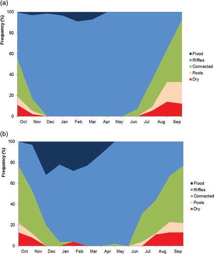
The SIMGRO model was run for a period of 9 years (2000–2008) to generate daily discharges. For each stream reach, defined as the major reaches in each sub-basin, a flow duration curve was calculated and the thresholds for the different aquatic states depending on local conditions were calculated. Data from the Vrontamas gauge (for location see Fig. 2) were used to verify the SIMGRO model results. Average monthly flow data were available from point measurements and manual interpolation. When measured discharges from a gauging station are available, the thresholds from Table 1 were based on visual interpretation of the aquatic states. The aquatic states frequency graph (ASFG) based on measurements (Gamvroudis et al. 2011) compares quite well with the ASFG based on model results. Figure 4(a) shows the ASFG based on SIMGRO model results, and derived from daily discharges. The daily-calculated flows are converted to averages per month. Figure 4(b) shows the ASFG derived from measured average monthly discharges. The differences are small, except between July and September when the model results for the connected state are larger than those based on measured data (Fig. 4(b)). The stream can be dry for as much as 20% of the time, especially between July and November (Fig. 4(a)). Pools occur mainly in autumn. From November to July the riverbed contains flowing water. The flood phase occurs about 5–10% of the time from December to April. The corresponding threshold discharges for the situation at Vrontamas are given in Table 2. These discharges apply to this reach only, since stream width and bed slope vary per stream reach.

Figure 4. Frequency of the considered flow phases for the Vrontamas gauge (a) SIMGRO, (b) derived from measured data.

The ASFG can be presented not only in time, as done in the previous graphs, but also in space. Within the GIS user interface AlterrAqua, the flow analysis and characterization was carried out for all streams in the Evrotas basin. Figure 5 shows a spatial representation of the different aquatic states for all major streams. Based on the average frequencies for the years 2000–2008, it appears that the main stream does not ever dry up completely, though the tributaries often do. The main river has the lowest dry state frequency. For the streams presented in Fig. 5, the duration of the aquatic states is on average 0.9% for floods, 15.1% for riffles, 22.6% for connected streams, 6.7% for pools and 54.7% for a dry streambed. The figure shows how these categories are distributed across the Evrotas basin, with large areas of temporary streams associated with karst recharge areas, and some of the permanent reaches associated with karstic springs. Such information can be used to derive the ecological status for the WFD.

Figure 5. Average frequency of the different flow phases for all major streams in the Evrotas basin, based on results of the SIMGRO model (simulation period 2000–2008).

There is a large amount of uncertainty in the model, mainly due to lack of data on the groundwater characteristics and the water use for irrigation by the farmers. As it is important to know how sensitive the model is to changes in the input data, we carried out a limited sensitivity analysis to investigate the sensitivity of the input data that had been modified most during this research. The parameters changed were transmissivity, crop factors and irrigation (Cazemier et al. 2011). The changes in river flows were small, but it was found that the aquatic states are sensitive to changes in the threshold values. Such changes and the overall uncertainty in the model need to be taken into account when interpreting the low flow characterization and scenarios.

4.3 Scenario analysis for historical situations and climate change

In the Evrotas basin, irrigation canals have been used since antiquity to transport water from the river and springs to irrigate agricultural fields and to provide people with water. The cultivated area has expanded since the mid-20th century as new crops were introduced (such as oranges) that require more irrigation, and therefore groundwater use has increased considerably. As a result, stretches of the Evrotas main channel and significant tributaries that used to maintain permanent flow now fall dry, with tremendous repercussions for the biota.

In order to assess the changes in the hydrological conditions in the Evrotas River basin we defined historical situations and a climate scenario for the near future to be analysed by the SIMGRO model. For the historical scenarios, the meteorological data were kept the same as for the present situation (2000–2008) in order to compare results. The historical scenarios give an indication of the changes in the flow regime during the past century, how flow conditions have changed over time and the consequences for aquatic life. They reveal the changes from the near-natural conditions a century ago to the human impact of the present situation. The future scenario indicates the changes in discharge regime and implementation of ecological measures that might happen because of climate change.

4.3.1 Historical scenarios

The three historical scenarios 1900, 1960 and 1980 defined by Vernooij et al. (2011) were the core years. These are scenarios for periods of 9 years around the three core years. In these scenarios, only the changes in the area of land use, irrigation intensity and the extraction groundwater and surface water were considered. The historical scenarios were constructed using data on changes in land use and irrigation as shown in Table 3. We compared the current situation (2000–2008) with the natural situation, to determine how human impact has affected the ecological status. We assumed that the scenario for the period around the year 1900 is the near-natural situation without major human influence. The small amount of irrigation water use before 1900 was considered to be included in the near-natural situation. The other scenarios (1960s and 1980s) mark periods in which major changes took place. For 1900, it was assumed that the agriculture area was about 30% less than the current situation. It was also assumed that the predominant land cover was deciduous forest and that irrigation from surface water extended only up to 2 km from the main river. The irrigation intensity was assumed about 80% lower than it is today (Table 3). For the 1960s scenario the cultivated area did not change, but it was assumed that there was irrigation from groundwater (phreatic aquifer) at an intensity 60% lower than today. In the 1980s, the use of irrigation water increased and water was extracted mainly from the second aquifer. Since the 1980s, olives and orange trees in this area, as in all countries around the Mediterranean Sea, have been irrigated to increase the yield.

Table 3. Change in cultivated area and irrigation intensity (relative to the present situation) adopted in the historical scenarios (Vernooij et al. 2011).

Period	Change cultiv.	Changes in irrigation	Irrigation intensity
	area (%)		(%)
1900	−30	Irrigation up to 2 km	−80
1960	−30	Irrigation also from groundwater	−60
1980	−20	Larger pumps and deeper abstraction	−40
Present	0	Olives are irrigated	0

4.3.2 Climate change scenario

The scenario defined for modelling the hydrology and ecological status in the Evrotas basin in the future considered climate change in terms of changes in precipitation, temperature and evapotranspiration based on the forecasts made by the IPCC (IPCC 2007). In this paper we present results for the climate scenario A2 for the Evrotas basin. This scenario is the worst-case situation and assumes maximum population growth, limited technological development and a rise in average annual temperature of between 2.0 and 5.4°C. The results for the B1 scenario have been reported elsewhere (Cazemier et al. 2011).

The A2 climate scenario assumes the Evrotas basin will experience a different climate in the future. Supit et al. (2012) provide an interpretation of three different climate model results, being from IPSL-CM4 (France), MICRO3.2 (Japan) and ECHAM5/MPI-OM (Germany). In our study the variables considered were the change in average monthly data from the climate models on precipitation and temperature. The reference evapotranspiration was derived from the climate models using the Penman equation (Supit et al. 2012). We used the delta change approach: the climate model gives per month a change in precipitation and a change in temperature. The monthly changes were used to convert the daily meteorological data for the period 2000–2008, to the 2050s, for precipitation, temperature and the reference evapotranspiration. This approach assumed that temporal and spatial rainfall distribution for the 9 years remain unchanged. The precipitation remains almost equal: on average the precipitation intensity decreases by 4% in summer and 7% in winter. The temperature is on average 2.2°C higher and the reference evaporation increases by 20% in summer and 60% in winter. In the scenario no changes in land use and irrigation intensity were considered

4.4 Results of the scenario analysis

The changes for the historical scenarios were about land use and irrigation amounts. For the climate change scenario, only the meteorological data were changed. Simulations were performed for 9 years, so that the results show the hydrological situations for the historical periods and the 2050s. The change in river flow at Vrontamas when the present situation is compared with 1900 and 1980 is shown in Fig. 6. The higher flows do not change much, but the low flows in summer decrease dramatically from 1900 onwards. Around 1900, the low flows vary between 1.5 and 2.5 m³ s^-1; in the 1980s the low flows vary between 0.7 and 1.5 m³ s^-1; and nowadays the low flows are between 0.0 and 0.3 m³ s^-1.

Figure 6. Simulated discharges at the Vrontamas gauge for 1900, 1980 and the present situation.

The average frequencies of the aquatic states in the historical and future scenarios are shown in Table 4. The values were calculated by averaging the aquatic state frequencies for each stream reach, taking the total stream length into account. The table shows that the largest difference between the frequencies of the aquatic states is between the current situation and the scenario for the 1980s. The percentage of time the stream network is in a flood state has hardly changed. The percentages for the riffles, connected pools and pools states have decreased, especially for riffles and connected pools. In the past, the stream network was in a dry state for a much lower percentage of the year; the most dramatic change was between the 1980s and present: from 37.0% to 54.7%, an increase of 17.7% (Table 4). For the 2050 scenario the average percentage of time that a stretch of river dries up every year increases from 54.7% to 60.4%. The changes due to climate change are less than the changes resulting from human impact.

Table 4. Average duration of aquatic states for the five scenarios for the Evrotas River and all tributaries.

Scenario	Average aquatic state (%)		Connected	Isolated	Dry
	Flood	Riffles	pools	pools
1900	1.0	22.9	33.8	8.5	33.9
1960	1.0	22.4	32.7	8.1	35.7
1980	1.0	22.0	31.8	8.2	37.0
Present	0.9	15.1	22.6	6.7	54.7
2050 (A2)	0.7	12.0	20.3	6.7	60.4

The changes as presented in Table 4 have consequences for the aquatic organism assemblages. Aquatic communities in the Evrotas basin have been experiencing increasingly dry conditions during the past few decades. The species composition will therefore have changed during the past years to more drought-tolerant species, at the cost of drought-sensitive species (Bonada et al. 2007). The drying of a river is a “pulse” disturbance as defined in Lake (2003). This means that the intensity of the impact of the disturbance increases over time, but not suddenly. This allows many invertebrates to adapt, because some (like Coleoptera and Heteroptera) are able to migrate between pools. The main concern is the impact of temporary streams on animals that live in the stream in spring (when a succession of pools and riffles exists). If this part of the water cycle is eliminated or reduced to a period of less than three months, most Reophilous species may disappear and there will be a significant loss of river biodiversity.

An important criterion for good ecological status is the duration of the dry period in spring and maximum periods during an entire year. In spring the criterion is no dry period longer than one month, and for all year round it is a period no longer than 3 months. These criteria were examined for each river reach and the 9 simulation years (2000–2008). The model results show that in some cases there are consecutive years in which both criteria are exceeded. It is unknown how many consecutive years with such long dry periods will result in unacceptable ecological conditions. Therefore, we assumed that river reaches in which the maximum length of both dry periods is exceeded for 5 or more of the 9 years are generally too dry to support viable populations of the fish species described before. In all years it is necessary that isolated pools remain in order for the fish to survive. The percentages of the stream network that exceed this flow conditions criterion are shown in Table 5 for all the scenarios. The situation in 1900 is assumed the benchmark for the near natural situation. It appears that in the scenario for 1900, 38% of the major tributaries already had no viable riverine aquatic assemblage (typical for a riffles state) because the streams were too dry in spring (ephemeral streams). Furthermore, 50% of the stream network had long dry periods throughout the year, which caused the aquatic communities to deteriorate and made it impossible to quantify the ecological state on the basis of the aquatic organisms (Munné and Prat 2011). This being the case, a viable and diverse aquatic ecological community is not expected and therefore the ecological status of these reaches should be assessed using terrestrial rather than aquatic invertebrates. Unfortunately the use of terrestrial invertebrates for measuring ecological status is still in its infancy (Steward et al. 2012). For the comparison of the 1900 and present scenarios, the percentage of river reaches that are too dry in spring increased from 38% to 58%. The percentage of the river network that is too dry all year is 29% higher than in 1900 (79% vs 50%). This agrees with the field observations of Gamvroudis et al. (2011) for the dry year of 2007 that 30% of the main stream had no flow up to June of 2007, and the river desiccation (percentage of the length of the main stream that was dry) reached almost 80% during the dry months (from August to November). The model results for the current scenario and the field observations indicate that 79% of the stream network currently may not be classified as having good ecological status based on the hydrological regime. The dry state of this part of the stream network is the result of human influence (intensified irrigation and abstraction of water for domestic supply). We estimated that for the 2050s, 68% of the length of river and streambed in the basin will be too dry during the spring period (i.e. exceed the “more than 4 out of 9 years” criterion). This is 9% more than the current situation. This percentage indicates the proportion of the stream network in which aquatic communities cannot develop viably in spring. During the year, 80% of the river reaches are too dry. This is not significantly different from the present situation. Thus for the climate scenario, the ecological status of the stream network for the whole year, particularly in summer, will not worsen in terms of the persistence of the aquatic states today, assuming other factors to remain constant, like the change in groundwater extractions.

Table 5. Percentage of river reaches that are too dry in spring and all year round (criteria of more than 4 out of 9 years).

Scenario	Dry periods in spring (1 month)	Dry periods all year (3 months)
	(%)	(%)
1900	38	50
1960	39	54
1980	40	56
Present	58	79
2050	67	80

5 Discussion

A physically-based model was used to simulate regional groundwater and surface water flow in a basin with spatially variable geo-hydrological conditions and land use. A sensitivity analysis revealed small changes in river flows when transmissivities, crop factors or irrigation rates were changed. Due to the size of the model, its spatial resolution and the resulting large number of parameters, the model could not be fully calibrated. However, an attempt has been made to find the best possible fit against the available measurements. Unfortunately, only monthly measured discharge data were available for most of the period. Other input data, such as the hydrogeology or crop characteristics, were also limited. This lack of data makes it hard to assess the reliability of the model. The uncertainty about the input data has consequences for the modelling results and for the findings on the river’s hydrological and ecological status. Although very little data is available on the groundwater it is important to include the groundwater component in the basin model, as otherwise it is impossible to estimate the response of the groundwater abstractions for irrigation to the change in river flow. In addition, it is necessary to have an accurate estimate of the groundwater recharge and of its temporal and spatial variability in order to calculate the interaction between groundwater and surface water. Incorporating both the surface water and the groundwater in the model makes it possible to assess temporary stream conditions in terms of the characteristics and persistence of the aquatic states within a river basin. In addition, the simulations can focus on the impact of change (e.g. in cultivated areas or in groundwater abstractions) on the extent of intermittent flow and thus on the ecological status of the streams. In that respect the SIMGRO model is a powerful tool for modelling the historical, present or future flow regime and for producing maps of the area drained by temporary streams. The study also shows that a hydrological model incorporated within a GIS makes it easier to relate flow regime characteristics to spatially distributed catchment characteristics or associated river flows (Fig. 5). Spatial differentiation into sub-basins can reveal regions with an excessive exploitation of the water resources. Such information can be used to give indications of the ecological status or to assess the effect of changes in, for example, land use or climate.

The threshold values derived for the flow characterization separated the discharge regime into five aquatic states. The thresholds between these aquatic states were calibrated against measured discharges. The aquatic state frequency graph (Fig. 4) allowed the stream regime to be rapidly assessed visually, based on model results. The analysis shows that all the major streams are dry for 33.8% of the year on average, as shown in Fig. 5. We considered thresholds for each stream based on specific site characteristics that were hydraulic criteria: flow resistance, bed slope and stream width. Further improvements are needed to quantify the thresholds for the aquatic states to be used based on a geomorphological classification and different roughness values for each stream reach. In addition, the overall uncertainty in the model needs to be taken into account in the interpretation of the low flow characterization and scenarios. The flow characterization for the current situation showed that a large part of the stream network is too dry to accommodate the development of a biodiverse riverine aquatic community throughout the year. Table 3 and Fig. 5 show that all flow regimes are present in the basin, but the stream flow is seasonal rather than permanent.

The Water Framework legislation requires all water bodies in the EU except those that have been heavily modified to have a good ecological (and therefore hydrological) status by 2015. Temporary streams are not adequately incorporated in the WFD, because the aquatic biology of these water bodies, even if they are pristine, may be different from reference permanent bodies due to the occurrence of dry spells. Besides, it should be taken into account how human impact has influenced the streamflow of the water body and particularly the temporal patterns of the dry periods. In the Evrotas basin, anthropogenic influence has resulted in the discharge in the main stream being too little in spring and/or summer to comply with the WFD.

6 Conclusions and recommendations

The analysis in this paper confirms that, due to the increased use of water for irrigation, the water resources in the Evrotas basin are overexploited. Since 1900, river discharges have fallen, particularly in summer, and parts of the mainstream bed are now temporary. The largest change is in the period between 1980 and the present and is mainly the result of irrigating olives. Comparing the current situation with the natural situation in the year 1900 leads to the conclusion that currently 79% of the stream network is in a poor hydrological and ecological condition due to human influence. This percentage will increase only slightly in response to future climate change. The main problem in the Evrotas basin is the poor ecological status resulting largely from the poor hydrological status. Unless former hydrological conditions can be reinstated, it will be impossible to restore the streams to their 1900 ecological status.

For the stream network in the Evrotas River basin to be sustainable under the WFD, water use must be reduced. Our study shows that the river basin should be brought back to a situation comparable to that of 1980 in terms of water use for irrigation, i.e. before olives were irrigated. Another way to arrive at a sustainable situation is to apply less irrigation water. Farmers currently apply much more water to their crops than is recommended in the Greek government’s Good Agricultural Practices guide of 2004 (Greek Ministry of Agriculture 2004). An effective way of reducing water use would be to get the farmers to follow the recommendations in the guide.

Our scenario analysis using different levels of water requirements for irrigation revealed the conditions for sustainable use of the water resources. The proposed method can therefore help not only to identify near-natural flow conditions in an ideal setting, but also to analyse measures to restore the hydrological system. Such assessment is important for heavily modified water bodies for which river basin management plans must be developed.

Disclosure statement

No potential conflict of interest was reported by the authors.

Funding

The study was carried out within the MIRAGE project, EC Priority Area “Environment (including Climate Change)” [contract number 211732]. This research was also supported by the Dutch Ministry of Economic Affairs, Agriculture and Innovation.

References

- Abbott, M.B., et al., 1986. An introduction to the European Hydrological System — systeme Hydrologique Europeen, “SHE”, 1: history and philosophy of a physically-based, distributed modelling system. Journal of Hydrology, 87, 45–59. doi:10.1016/0022-1694(86)90114-9
- Acreman, M.C. and Ferguson, A.J.D., 2010. Environmental flows and the European water framework directive. Freshwater Biology, 55, 32–48. doi:10.1111/j.1365-2427.2009.02181.x
- Allen, R.G., et al., 1998. Crop evapotranspiration—Guidelines for computing crop water requirements. FAO, Rome, Italy. Paper 56.
- Arnold, J.G., et al., 1998. Large area hydrologic modeling and assessment Part I: model development. Journal of the American Water Resources Association, 34 (1), 73–89. doi:10.1111/j.1752-1688.1998.tb05961.x
- Bergsma, T., Querner, E.P., and Van Lanen, H.A.J., 2010. Studying the Rhine basin with SIMGRO; Impact of climate and land use changes on discharge and hydrological droughts. Wageningen, Alterra, Alterra Report 2082. 45 pp.
- Bonada, N., Rieradevall, M., and Prat, N., 2007. Macroinvertebrate community structure and biological traits related to flow permanence in a Mediterranean river network. Hydrobiologia, 589, 91–106. doi:10.1007/s10750-007-0723-5
- Boulton, A.J., 2003. Parallels and contrasts in the effects of drought on stream macro invertebrate assemblages. Freshwater Biology, 48, 1173–1185.
- Bull, L.J. and Kirkby, M.J., 2002. Dryland river characteristics and concept. In: L.J. Bull and M.J. Kirkby, eds. Dryland rivers: hydrology and geomorphology of semi-arid channels. Chichester, UK: John Wiley & Sons Ltd, 4–15.
- Camporese, M., et al., 2010. Surface-subsurface flow modeling with path-based runoff routing, boundary condition-based coupling, and assimilation of multisource observation data. Water Resources Research, 46, W02512. doi:10.1029/2008WR007536
- Cazemier, M.M., et al., 2011. Hydrological analysis of the Evrotas basin, Greece; Low flow characterization and scenario analysis. Wageningen, Alterra, Alterra report 2249, 57.
- Chen, X., Chen, Y.D., and Zhang, Z., 2007. A numerical modeling system of the hydrological cycle for estimation of water fluxes in the Huaihe River Plain Region, China. Journal of Hydrometeorology, 8, 702–714. doi:10.1175/JHM604.1
- Chow, V.T., 1959. Open channel hydraulics. New York, NY: McGraw Hill.
- Datry, T., Arscott, D.B., and Sabater, S., 2011. Recent perspectives on temporary river ecology. Aquatic Sciences, 73 (4), 453–457. doi:10.1007/s00027-011-0236-1
- Ebel, B.A., et al., 2009. First-order exchange coefficient coupling for simulating surface water–groundwater interactions: parameter sensitivity and consistency with a physics-based approach. Hydrological Processes, 23, 1949–1959. doi:10.1002/hyp.7279, doi:10.1002/hyp.6642
- Ernst, L.F., 1978. Drainage of undulating sandy soils with high groundwater tables. Journal of Hydrology, 39, 1–50. doi:10.1016/0022-1694(78)90111-7
- Freeze, R.A. and Harlan, R.L., 1969. Blueprint for a physically-based, digitally-simulated hydrologic response model. Journal of Hydrology, 9, 237–258. doi:10.1016/0022-1694(69)90020-1
- Froebrich, J., et al., 2010. Visions for water management. International Innovation: Environment Oct. 2010, 82–84. Available from www.iwrm.wur.nl.
- Gallart, F., et al., 2008. Investigating hydrological regimes and processes in a set of catchments with temporary waters in Mediterranean Europe. Hydrological Sciences Journal, 53, 618–628. doi:10.1623/hysj.53.3.618
- Gallart, F., et al., 2012. A novel approach to analysing the regimes of temporary streams in relation to their controls on the composition and structure of aquatic biota. Earth System Sciences, 16, 3165–3182. Available from: www.hydrol-earth-syst-sci.net/16/3165/2012/10.5194/hess-16-3165-2012.
- Gamvroudis, C., et al., 2011. Hydrograph Analysis of Oinountas river basin. In: N. Lambrakis, G. Stournaras, and K. Katsanou, eds. Advances in the research of aquatic environment, environmental earth sciences. Berlin: Springer. ISBN: 978-3-642-19902-8, 171–178. doi:10.1007/978-3-642-19902-8_19
- Gasith, A. and Resh, V.H., 1999. Streams in Mediterranean climate regions: abiotic influences and biotic responses to predictable seasonal events. Annual Review of Ecology and Systematics, 30, 51–81. doi:10.1146/annurev.ecolsys.30.1.51
- Greek Ministry of Agriculture, 2004. Good Agricultural Practices (G.A.P. 40/2004). In agreement to the decision Ε(2003)3139/22-8-2003 of EE.
- Grindlay, A.L., et al., 2011. Implementation of the European Water Framework Directive: integration of hydrological and regional planning at the Segura River Basin, southeast Spain. Land Use Policy, 28 (1), 242–256. doi:10.1016/j.landusepol.2010.06.005
- IPCC, 2007. Climate Change 2007: Synthesis Report. Contribution of Working Groups I, II and III to the Fourth Assessment Report of the Intergovernmental Panel on Climate Change [Core Writing Team: Pachauri, R.K and Reisinger, A. (eds.)]. IPCC, Geneva, Switzerland.
- Kennard, M.J., et al., 2010. Classification of natural flow regimes in Australia to support environmental flow management. Freshwater Biology, 55, 171–193. doi:10.1111/j.1365-2427.2009.02307.x
- Kollet, S.J. and Maxwell, R.M., 2006. Integrated surface–groundwater flow modeling: a free-surface overland flow boundary condition in a parallel groundwater flow model. Advances in Water Resources, 29 (7), 945–958. doi:10.1016/j.advwatres.2005.08.006
- Lake, P.S., 2003. Ecological effects of perturbation by drought in flowing waters. Freshwater Biology, 48, 1161–1172. doi:10.1046/j.1365-2427.2003.01086.x
- Larned, S.T., et al., 2010. Emerging concepts in temporary-river ecology. Freshwater Biology, 55 (4), 717–738. doi:10.1111/j.1365-2427.2009.02322.x
- Lytle, D.A. and Poff, N.L., 2004. Adaptation to natural flow regimes. Trends in Ecology and Evolution, 19, 94–100. doi:10.1016/j.tree.2003.10.002
- Magalhães, M.F., et al., 2007. Effects of multi-year droughts on fish assemblages of seasonally drying Mediterranean streams. Freshwater Biology, 52, 1494–1510. doi:10.1111/j.1365-2427.2007.01781.x
- MIRAGE, 2012. Mediterranean Intermittent River ManAGEment: Periodic report period July 2010–December 2011, Wageningen, Alterra, The Netherlands.
- Moraetis, D., et al., 2010. High-frequency monitoring for the identification of hydrological and bio-geochemical processes in a Mediterranean river basin. Journal of Hydrology, 389, 127–136. doi:10.1016/j.jhydrol.2010.05.037
- Munné, A. and Prat, N., 2011. Effects of Mediterranean climate annual variability on stream biological quality assessment using macro invertebrate communities. Ecological Indicators, 11, 651–662. doi:10.1016/j.ecolind.2010.09.004
- Nash, J.E. and Sutcliffe, J.V., 1970. River flow forecasting through conceptual models. Part I – a discussion of principles. Journal of Hydrology, 10, 282–290. doi:10.1016/0022-1694(70)90255-6
- Poff, N.L., 1996. A hydro geography of unregulated streams in the United States and an examination of scale-dependence in some hydrological descriptors. Freshwater Biology, 36, 71–79. doi:10.1046/j.1365-2427.1996.00073.x
- Povilaitis, A. and Querner, E.P., 2006. Analysis of water management measures in the Dovine River Basin, Lithuania Possibilities to restore a natural water regime. Wageningen, Alterra, Alterra-rapport 1370, 67.
- Querner, E.P., 1986. An integrated surface and groundwater flow model for the design and operation of drainage systems. Int. Conf. on Hydraul. Design in Water Res. Eng.: Land Drainage, Southampton, 101–108.
- Querner, E.P., 1997. Description and application of the combined surface and groundwater flow model MOGROW. Journal of Hydrology, 192, 158–188. doi:10.1016/S0022-1694(96)03107-1
- Querner, E.P., Morábito, J.A., and Tozzi, D., 2008. SIMGRO, a GIS-supported regional hydrologic model in irrigated areas: case study in Mendoza, Argentina. Journal of Irrigation and Drainage Engineering, 134 (1), 43–48. doi:10.1061/(ASCE)0733-9437(2008)134:1(43)
- Querner, E.P. and Povilaitis, A., 2009. Hydrological effects of water management measures in the Dovinė River Basin, Lithuania. Hydrological Sciences Journal, 54 (2), 363–374. doi:10.1623/hysj.54.2.363
- Querner, E.P. and Van Lanen, H.A.J., 2010. Using SIMGRO for drought analysis – as demonstrated for the Taquari Basin, Brazil. In: E. Servat, et al. eds, Global change: facing risks and threats to water resources (Proc. of the Sixth World FRIEND Conference, Fez, Morocco, Oct. 2010). Wallingford, UK: International Association of Hydrological Sciences IAHS Publ. 340, 111–118.
- Skoulikidis, N., et al., 2010. Differences between natural and created desiccation in the management of temporary river basins–the Evrotas River case study. BALWOIS Conf. May 2010. Ohrid, Republic of Macedonia.
- Skoulikidis, N., et al., 2011. Assessing water stress in Mediterranean lotic systems: insights from an artificially intermittent river in Greece. Aquatic Science, 73, 581–597. doi:10.1007/s00027-011-0228-1
- Steward, A.L., et al., 2012. When the river runs dry: human and ecological values of dry riverbeds. Frontiers in Ecology and the Environment, 10 (4), 202–209. doi:10.1890/110136
- Supit, I., et al., 2012. Climate change effects on European agricultural production. Journal of Agricultural and Forest Meteorology. doi:10.1016/j.agrformet.2012.05.005
- Tzoraki, O., et al., 2013. Flood generation and classification of a semi-arid intermittent flow watershed: Evrotas river. International Journal of River Basin Management, 11 (1), 77–92. doi:10.1080/15715124.2013.768623
- Tzoraki, O., et al., 2011. Hydrologic modelling of a complex hydrogeologic basin: Evrotas River Basin. In: N. Lambrakis, G. Stournaras, and K. Katsanou, eds. Advances in the research of aquatic environment; environmental earth sciences. Springer Berlin Heidelberg. ISBN: 978-3-642-19902-8, 179–186. doi:10.1007/978-3-642-19902-8_20
- Uys, M.C. and O’Keeffe, H., 1997. Simple words and fuzzy zones: early directions for temporary river research in South Africa. Environmental Management, 21 (4), 517–531. doi:10.1007/s002679900047
- Vardakas, L., et al., 2010. Assessing the ecological status of the “artificially intermittent” Evrotas River (Greece) according to the Water Framework Directive 2000/60/EC. BALWOIS Conf. May 2010. Ohrid, Republic of Macedonia.
- Vernooij, M., et al., 2011. Flow characterization temporary streams: Using the model SIMGRO for the Evrotas basin, Greece. Alterra, Wageningen, Alterra-report 2126, 60 pp.
- White, W.B., 2003. Conceptual models for karstic aquifers. Speleogenesis and Evolution of Karst Aquifers, 1, 1.
- Wriedt, G., et al., 2009. Estimating irrigation water requirements in Europe. Journal of Hydrology, 373, 527–544. doi:10.1016/j.jhydrol.2009.05.018