Forecasting streamflow by combination of a genetic input selection algorithm and wavelet transforms using ANFIS models

ABSTRACT

In this study, a data-driven streamflow forecasting model is developed, in which appropriate model inputs are selected using a binary genetic algorithm (GA). The process involves using a combination of a GA input selection method and two adaptive neuro-fuzzy inference systems (ANFIS): subtractive (Sub)-ANFIS and fuzzy C-means (FCM)-ANFIS. Moreover, the application of wavelet transforms coupled with these models is tested. Long-term data for the Lighvan and Ajichai basins in Iran are used to develop the models. The results indicate considerable improvements when GA selection and wavelet methods are used in both models. For example, the Nash-Sutcliffe efficiency (NSE) coefficient for Lighvan using FCM-ANFIS is 0.74. However, when GA selection is applied, the NSE is improved to 0.85. Moreover, when the wavelet method is added, the performance of new hybrid models shows noticeable enhancements. The NSE value of wavelet-FCM-ANFIS is improved to 0.97 for Lighvan basin.

Editor D. Koutsoyiannis Associate editor E. Toth

KEYWORDS:

• ANFIS
• wavelet transform
• streamflow forecasting
• genetic algorithm
• input selection

1 Introduction

An accurate forecast of high and low streamflow can provide information for water resources management, policy decision making and city planning. Streamflow forecasting is a difficult task in hydrology because of the wide range of variability in scales of both space and time. However, artificial intelligence (AI) techniques are known to have great capabilities in forecasting nonlinear hydrological time series. There has been a growing interest in using AI methods for a wide variety of engineering problems for the last two decades. These methods employ the available historical time series for simulating the hydrological systems and, in this respect, artificial neural networks (ANN) and adaptive neuro-fuzzy inference systems (ANFIS) have been at the centre of attention for developing data-driven hydrological models.

Many researchers have used neural networks in various hydrological studies (e.g. Zealand et al. 1999, Wang et al. 2006, Sattari et al. 2012, Zounemat-Kermani 2013). ANFIS, which is ANN coupled with a fuzzy system, holds the advantages of both ANN and fuzzy systems and has been used as a substitute for ANN in many applications. Recently, there have been many applications of ANFIS in various water resources problems, such as river flow forecasting (Bea et al. 2007), and evaporation and evapotranspiration estimates (Cobaner 2011, Sanikhani et al. 2012). In most of such studies, ANFIS and ANN methods are compared, and usually ANFIS has been indicated as the superior method. For example, Nayak et al. (2004) compared the application of ANFIS with ANN and autoregressive moving average (ARMA) methods for modelling the streamflow of the Baitarani River in India. According to their results, ANFIS performed better than both ANN and traditional ARMA models. Chang and Chang (2006) applied ANFIS for short-term prediction of the Shihmen Reservoir water level in Taiwan. They used human decision (i.e. current reservoir operation outflow) as input variable and their results showed more improvement than the method without using this parameter. Using various combinations of climate variables, Kişi (2006) investigated the application of ANFIS to model daily pan evaporation, indicating the superiority of ANFIS over neural networks in his application. Bae et al. (2007) developed an ANFIS model based on subtractive clustering for monthly reservoir inflow forecasting using past observed data and future forecasted weather information as inputs. Their results revealed that ANFIS based on subtractive clustering was appropriate for inflow forecasts. Also, Cobaner (2011) estimated reference crop evapotranspiration using two different neuro-fuzzy systems based on grid partition and subtractive clustering. The results of subtractive clustering-based fuzzy inference systems showed slightly better performance than the grid partition-based fuzzy inference systems.

An important issue with most of the data-driven methods, including ANN and ANFIS, is the proper selection of input data, as well as other concerns such as model topology. It is now well known that the proper selection of input variables has a fundamental impact on the performance of data-driven models. A review of the literature in streamflow forecasting fields reveals that researchers usually selected input variables subjectively through their experience, or, in most cases, through a limited trial-and-error method. Neither of these methods is reliable and consistent when dealing with large multivariable problems.

Selecting the optimal subset within available datasets can lead to better description of model output. Zhang and Hu (2005) used a binary particle swarm optimization algorithm to select optimal input variables for a support vector machine (SVM). They applied this method in forecasting a real financial time series and indicated better generalization and higher rate of convergence of the model. Khazaee et al. (2008) presented a genetic-based optimal input selection method to choose input variables for a wavelet neural network prediction model. They applied their proposed model to predict a time series and showed that input selection by genetic algorithm (GA) is better than other selection methods such as correlation analysis or the Gamma test.

There are also some applications of input selection algorithms in the water resources area. For example, Bowden et al. (2005) investigated appropriate input variables selection in water resources, using two input determination approaches including partial mutual information (PMI) to select important model inputs, and the hybrid GA and general regression neural network to reject redundant input variables. They found effective inputs to forecast salinity for the River Murray in Australia, and indicated that both input determination techniques improved their results, but the developed ANNs using PMI were found to be the most robust models. Fernando et al. (2009) also applied PMI to identify suitable inputs to forecast salinity in the River Murray. Their results indicated that the ANN models developed by an input selection process perform better than those not using this process. Noori et al. (2011) applied a combination of an input selection approach and the SVM model for monthly streamflow prediction. They investigated the effect of three input selection methods, including principal component analysis, Gamma test and forward selection methods, on the SVM model performance. They demonstrated that the results of the SVM model developed by principal component analysis and the Gamma test are better than the original SVM model. Asadi et al. (2013) proposed a combination of data pre-processing and ANN to predict runoff at the Aghchai watershed in Iran. They used stepwise regression analysis to select the best input variables and demonstrated that input selection had a positive impact on their results.

Nevertheless, most input variable selection approaches in water resources deal with ANN models. There are also a few studies that deal with ANFIS applications. For example, Moghaddamnia et al. (2009) used a Gamma test input selection method in developing ANN and ANFIS models to estimate evaporation in a hot and dry climate. Their results showed that the Gamma test has the capability of saving time and effort in selecting the best input variables. Also, Jeong et al. (2012) applied a neuro-fuzzy model to forecast monthly precipitation. They showed that using a wrapper method for feature selection and removing irrelevant input variables can lead to reduction of the uncertainties in forecasting.

Regardless of their successful applications, both ANN and ANFIS face some deficiencies, especially in association with non-stationary signals forecasting. In other words, when signal fluctuations are non-stationary, the precision of forecasting approaches is not satisfactory. Therefore, the model performs poorly under these circumstances. Recently, wavelet transform has been used to overcome this deficiency, and through its successful applications it has become a popular tool in enhancing the performance of data-driven models. It does this through explaining both spectral and temporal information in signals. There has been a growing tendency towards using wavelet transform methods in recent years (e.g. Szu et al. 1996, Lefebvre et al. 2000, Dai et al. 2003, Peng and Chu 2004). Some have developed hydrological forecasting models using ANN and wavelet method (e.g. Kim and Valdés 2003, Rajaee et al. 2011, Wei et al. 2013, Santos and Silva 2014), while others have investigated combining ANFIS and wavelet method to develop hybrid models with hydrologic applications (e.g. Partal and Kişi 2007, Shiri and Kisi 2010, Nourani et al. 2011, Kisi and Shiri 2012). Santos and Silva (2014) compared the performance of single ANN and wavelet-ANN models for 1- to 7-day-ahead streamflow forecasting. They demonstrated that using the wavelet method improves daily forecasting, especially for longer lead times (i.e. 5- and 7-day-ahead forecasts). In addition, they employed a trial-and-error process for selecting appropriate input variables. Their results showed that using the approximations of the first five decomposition levels as inputs produced the best results, and incorporation of detailed signals did not directly play an important role in improving the results. Partal and Kişi (2007) used a combination of discrete wavelet transform and a neuro-fuzzy model to forecast daily precipitation in Turkey. They used discrete wavelet transform to decompose precipitation signals into sub-signals and then applied the appropriate sub-signals as input of the neuro-fuzzy model to predict daily precipitation. According to their comparison, the model using wavelet transform indicates better results than the one without. Shiri and Kisi (2010) also investigated the accuracy of using neuro-fuzzy and wavelet-neuro-fuzzy models in predicting daily, monthly and annual streamflows, and showed that wavelet transform improves the results, especially in the annual model. Also, Kisi and Shiri (2012) demonstrated that the wavelet-neuro-fuzzy model was a superior alternative for forecasting short-term groundwater depths. They applied a correlation analysis between decomposed time series (detailed and approximate signals) and original current depth data and eliminated the signals with low correlation values.

In this study, two different neuro-fuzzy inference systems, namely subtractive (Sub)-ANFIS and fuzzy C-means (FCM)-ANFIS are compared in developing a nonlinear relationship between precipitation and streamflow of basins. Two sub-basins of different size within the Urmia Lake basin were chosen for developing and testing the ANFIS models. The ANFIS models with the whole set of input variables were used as a benchmark for comparison with the proposed models. In order to avoid noise in the model output and to obtain more reliable models, it is necessary to select proper inputs in data-driven models. Furthermore, selecting appropriate input variables (i.e. rain-gauges, temperature stations etc.) for these models can boost their performance, especially in large basins where determination of the input variables could become a challenging task. So, the application of the binary GA input selection algorithm is assessed on improving the streamflow forecasts in the basins by ANFIS models. Finally, to explore hidden characteristics of the time series, the application of discrete wavelet transform in conjunction with optimal data selection method and ANFIS models is investigated.

2 Methods

A brief review of methods applied in this paper is given below. More detailed explanation can be found in the cited literature.

2.1 Adaptive neuro-fuzzy inference system

Neuro-fuzzy simulation is a powerful method with capabilities based on neural networks. ANFIS uses neural network training methods and employs fuzzy logic to fit a relationship between some input space to output space. In other words, the parameters of fuzzy systems are fitted by neural network training algorithms (for more information see Jang 1993). It should be noted that subtractive and FCM clustering methods provide some information to obtain initial rules and fuzzy structure for generating the fuzzy inference system (Cobaner 2011). Then, fuzzy inference systems based on these clustering methods can provide a powerful model for making relationships between inputs and the output space. The subtractive and FCM-ANFIS models employed in this study are explained in detail below.

2.1.1 Subtractive clustering method

The purpose of clustering is to determine a comprehensive presentation of data behaviour (Chiu 1997). Yager and Filev (1994) presented the mountain method for clustering; then Chiu (1994) introduced subtractive clustering as a modified form of the mountain method. Subtractive clustering is a fast and one-pass algorithm for determining the number of clusters and cluster centres in data training spaces. In this method the potential of being a cluster centre is calculated for each data point and finally the data with highest potential values are selected as the cluster centres. Then, by determining the optimal value of the radius, the number of clusters is specified.

First the potential of being a cluster centre and its value P_i is calculated for each data point x_i by (Chiu 1994):

(1)

where m is the number of data points; and

(2)

where r_a is a positive constant value, and is effectively the radius for defining a neighbourhood; data points outside this radius have little influence on the potential value, so a data point with many neighbouring data points has a high potential of being cluster centre.

After computing the potential value of each data point, a data point with the highest potential value is selected as the first cluster centre. Then, in the second step, the potential of each data point P_i is updated by (Chiu 1994):

(3)

where x₁* and P₁* are the location of first cluster centre and its potential value, respectively. Also:

(4)

In equation (3) the potential value of the ith data point is a function of its distance from the first cluster centre. So, data points near the cluster centre have smaller potential values. In equation (4) r_b is a positive constant value that is effectively the radius defining a neighbourhood for which considerable potential reduction will happen. To avoid cluster centres being close to each other, r_b must be greater than 1.25 times r_a (Chiu 1994). When the potential of all data points has been computed according to equation (3), the highest remaining potential value is selected as the second cluster.

Generally, after obtaining the kth cluster centre, the potential of each data point is obtained by:

(5)

where P_k* is the highest potential value of cluster centre x_k (Chiu 1994). Also, to avoid marginal cluster centres the following criteria are used:

• If P_k* > e₁P₁*

• x_k* is the cluster centre and the cluster process is continued.

• Else if P_k* < e₂P₁*

• x_k* is not the cluster centre and the cluster process is ended

• Else

• x_k* is the cluster centre and the algorithm process is continued.

• Else

• x_k* is not the cluster centre and potential centre of x_k*set to 0 and then the data point with the next highest potential is set as the new x_k* and test again.

• End if

• End if

In his article, Chiu (1994) used e₁ = 0.5 and e₂ = 0.15; d_min is the shortest distance between x_k* and all previously found cluster centres.

2.1.2 Fuzzy C-means clustering method

The FCM clustering method was initially introduced by Bezdek (1973). In the FCM method, by having the specific number of clusters in hand, the cluster centres are determined in data point spaces and then each data point is assigned to a cluster by a specified membership degree.

The method uses an iterative algorithm with the objective to minimize the following function:

(6)

where y = {y₁, y₂, …, y_N} is the set of data points, c is the number of clusters (2 ≤ c < n), N is the number of data points, m is a real number (1 ≤ m < ∞), and u_ik is membership degree of y_k in the ith cluster. The parameters U and V of the objective function J_m are described below.

There are two main parameters in the objective function that present membership degree and cluster centre. Parameter U = [u_ik], which is a c × n matrix, presents membership degree of each data point. Values in the ith row show membership degree of data points in the ith cluster and values in the kth column show membership degree of the kth data point in all clusters. All values of u_ik are in the range [0,1]. Also, the following conditions must be established:

(7)

(8)

The other main parameter of the objective function is V = {υ₁, υ₂, …, υ _i} which presents the cluster centres.

Optimal clustering of data points is determined by two matrixes U and V. In other words, parameters that minimize the objective function produce the optimal clustering. To minimize the above objective function (equation (6)), iterative action to update u_ik and v_i is carried out using the following relationships (Bezdek 1973):

(9)

(10)

To start with the algorithm, values of c and m are set and then the initial membership degree matrix is fixed. In the next step, values of υ_i are computed by equation (9) and then u_ik is updated by equation (10). If the difference between u_ik in steps k and k + 1 is smaller than a specified value, the algorithm is ended; otherwise the updated u_ik (obtained by equation (10) in step k + 1) is set as the new value of u_ik and equations (9) and (10) are repeated (Bezdek 1973).

2.2 Input variable selection methods

Input variable selection approaches are classified into three groups: wrapper, embedded and filter methods. In wrapper methods, subsets of inputs are searched through the space of candidate inputs by using a search strategy (i.e. genetic algorithm). Each subset is used to train a predictor model (e.g. ANFIS) and to test the trained model using an independent set of data. In this way, each subset is assessed and the subset that causes the optimal generalization performance of the trained model is selected.

Embedded methods are a direct part of the machine learning algorithm. According to the impact of inputs on the model performance, the corresponding weights are adjusted so that the optimal structure of the predictor model is formed (e.g. ANFIS). In this way, the irrelevant and redundant weights are progressively removed. Unlike the wrapper and embedded approaches, filter methods are independent of the machine learning algorithm. In this approach, the important input variables are highlighted by the measure of their relevance by means of some factor such as mutual information. For more comprehensive information on these three input variable selection approaches, readers are referred to Kohavi and John (1997), Blum and Langley (1997) and Guyon and Elisseeff (2003). In this study, the wrapper method was used to select optimal input variables. Selection of input variables by genetic algorithm (GA) is presented in detail in the next subsection.

2.2.1 Genetic input selection algorithm

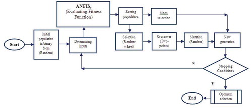
As explained in Fig. 1, the GA input selection algorithm applied herein begins by generating a random binary population. The population consists of a certain number of chromosomes with binary structure. In binary GA, each variable is represented by a zero/one parameter by a single bit. A value of 1 means that the variable should be included in the forecasting model, while a zero means that the variable should be excluded. After input variables have been determined through the assumed binary rule, they are used as inputs of the ANFIS model where the fitness function of each chromosome is calculated. The population is sorted according to evaluated fitness functions of chromosomes, after which elite chromosomes are selected for the next generation. Meanwhile, for the remaining chromosomes the main GA operators including selection (roulette wheel), crossover (two-point), and mutation (random) are applied and the new generation is produced. Then stopping conditions (either a certain number of iterations or achieving a specific value) are checked and a decision is made to continue the loop or to end the process. If conditions are satisfied, the process is ended. Otherwise, the new inputs are determined using the produced generation and the iteration is repeated as shown in Fig. 1. To maintain the effective individuals, the rate of elitism is assumed to be 0.1%, where, after selecting elite chromosomes, they are directly transformed to the next generation. In this study, crossover and mutation rates are assumed to be 0.70 and 0.001, respectively. In addition, using a trial-and-error process, the numbers of population and total generations are respectively found to be 20 and 150.

Figure 1. Flowchart of input selection method.

2.3 Wavelet transform

Wavelet transform, which is a relatively new progression in the field of signal processing, has attracted much attention since its introduction in the early 1980s. The first aim of wavelet analysis includes determination of both the frequency content of a signal and the temporal variation of this frequency content. Therefore, the wavelet transform is considered a useful choice when signals are characterized by localized high frequency events. There are two main categories of wavelet transform: continuous (CWT) and discrete (DWT). The first deals with continuous functions and the second is applied for discrete functions or time series. Most hydrological time series (i.e. precipitation and streamflow) are measured in discrete time steps; therefore, DWT would be a suitable method for decomposition and reconstruction of these series.

Wavelet transform converts a main signal to some wavelets (φ_a,_τ(t)), which can be obtained by compressing and expanding the mother wavelet:

(11)

where φ(t) is the wavelet function or mother wavelet, a is a scale or frequency factor also called the dilation factor, and τ is the time factor. The term “scale” refers to extending or compressing the wavelet. Using a small scale causes the wavelet to be compressed and in the case of a large scale the wavelet is extended. Large-scale values are not able to show details whereas small scales are applied to reveal more details.

The time-scale wavelet transform of continuous time series, x(t), is defined as (Mallat 1998):

(12)

where * denotes a conjugate complex function. Other terms are as defined earlier.

Continuous wavelet transform (CWT) needs wavelet coefficients to be calculated at each scale, which requires more calculations and computer time. In contrast, the discrete wavelet transform (DWT) requires less computation time and is simpler to develop (Adamowski and Chan 2011). Discrete wavelets have the following general form (Grossman and Morlet 1984):

(13)

where m and n are integers that control, respectively, the wavelet dilation and translation; a₀ is a specified fixed dilation step with a value greater than 1; and τ₀ is the location parameter which must be greater than zero. Scales and positions are usually based on powers of 2 (dyadic scales and positions), making it more efficient for practical cases (Mallat 1998). The most common (and simplest) choices for the parameters a₀ and τ₀ are 2 and 1, respectively. In this way, for a discrete time series x_i, which occurs at different time t, the DWT is defined as (Mallat 1998):

(14)

where W_m,n is the wavelet coefficient for the discrete wavelet of scale a = 2^m and location τ = 2^mn.

The discrete wavelet transform is used to decompose the time series data and by this procedure the signal is divided into two parts including “approximation” and “details”. In this way, the original signal is broken down into lower resolution components. These components explain behaviour better and reveal more information about the process than the original time series. Therefore, they can help the forecasting models to predict with more accuracy (Remesan et al. 2009, Calatao et al. 2011).

3 Case study

The data used for developing and testing the models are provided from two sub-basins of the Urmia Lake basin, which is located within two Azerbaijan provinces in northwest Iran and has an area of 51 876 km² (Fig. 2). The western limits of the basin overlap the elevations on the border between Iran and Turkey. The Urmia Lake located at the centre of the closed Urmia basin and west of the Caspian Sea is one of the most important and valuable ecosystems in the country and probably one of the unique basins of the world. The two sub-basins are Lighvan, with an area of about 186 km² a small basin located in the heights of Mount Sahand, and Ajichai, with an area of over 7600 km², considered a relatively large basin located northeast of the lake. A monthly time step was selected as the time interval in developing the forecasting models in this research.

Figure 2. Lighvan and Ajichai sub-basins in the Urmia Lake basin, Iran.

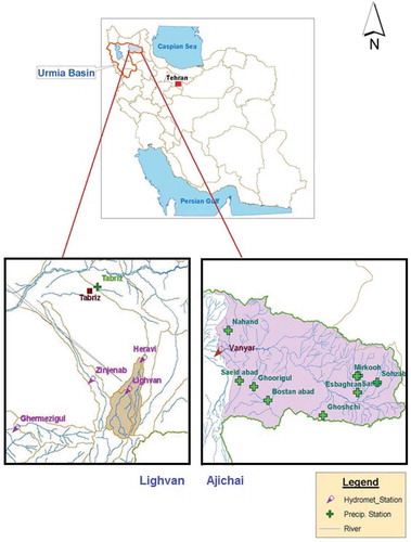
At the Lighvan outlet, the Heravi hydrometric station receives discharge from an area of 186.3 km². Precipitation at three raingauge stations in the nearby area (Tabriz, Ghermezigul and Zinjenab) and temperature measurements at Lighvan are used in developing streamflow forecasting models for the Lighvan sub-basin. The Vanyar hydrometric station receives streamflow from an area of 7675 km² at the outlet of the Ajichai sub-basin. Precipitation stations considered for this basin are: Bostanabad, Ghurigul, Ghushchi, Nahand, Saeedabad, Sarab, Sbaghran, Sohzab and Vanyar. In addition, temperature data from Sohzab, Mirkuh and Ghurigul stations are used for developing the streamflow forecasting models. For all stations, 41 years (1966–2006, inclusive) of monthly data are available, of which 85% (417 months) are used for training the models and the remaining 15% (75 months) are applied for testing the models. The training data should have the maximum and minimum observations for better training of the model. The common practice is to assign the first 85% (or any other proportion) for training and the last portion for testing the model. However, in the Ajichai sub-basin the observed maximum lies in the last 15% of the data. Therefore, the data for the test period are chosen from a middle section in order to have the observed maximum in the training process. So, after an initial assessment, the test period data were chosen from the last and middle parts of the dataset for Lighvan and Ajichai sub-basins, respectively.

The models are evaluated through three well-known criteria, as presented in Table 1.

Table 1. Forecasting accuracy criteria.

Criterion	Formula	Definitions
Coefficient of determination (R^2)		Qobs: observed
		Qpred: predicted
Root mean square error (RMSE)		: mean observed
		: mean predicted
Nash-Sutcliffe model efficiency (NSE)

N: number of data; Parameter ranges: 0 ≤ R² ≤ 1; 0 ≤ RMSE ≤ ∞; −∞ ≤ NSE ≤ 1.

In forecasting models NSE gives a better measure for the goodness of forecasts. The coefficient of determination by itself could mislead one by showing high values where predicted flows are very different but highly correlated with observed ones. The RMSE could help to partly overcome this problem but it lacks a firm measure of model accuracy because its value is data scale dependent. The NSE is dimensionless and free of scale and has been widely used in hydrology and other fields of science since it was introduced by Nash and Sutcliffe (1970).

4 Results and discussion

4.1 Basic models

Basic ANFIS models (Sub- and FCM-ANFIS) without any data pre-processing were used to forecast the basin streamflow. All the available input variables—without applying the selection algorithm—were employed, as follows:

• Input variables of Lighvan basic model: P_Tabriz, P_Ghermezigul, P_Zinjenab, T_Lighvan, Q_Heravi; all with 1 and 2 lags (total of 10 parameters).

• Input variables of Ajichai basic model: P_Bostanabad, P_Ghurigul, P_Ghushchi, P_Nahand, P_Saeedabad, P_Sarab, P_Sbaghran, P_Sohzab, P_Vanyar, T_Sohzab, T_Mirkuh, T_Ghurigul and Q_Vanyar; all with 1 lag time (13 parameters).

It should be noted that in the case of the Ajichai sub-basin the variables using lag 2 (i.e. t – 2) were omitted for simplicity and for keeping the number of parameters in a limited range.

In the next step, the final architecture of the ANFIS model including some parameters of Sub- and FCM-ANFIS methods was obtained through a trial-and-error process. Through this process the optimal radius for generating fuzzy rules is determined in the Sub-ANFIS model. This parameter determines the effective range of each cluster; small radiuses produce many small clusters and a large number of fuzzy rules, while large radiuses produce a few large clusters and a small number of fuzzy rules (Cobaner 2011). Too large or small radiuses are not suitable for clustering purposes, so they cannot properly introduce data spaces. Therefore, the optimal value of this parameter should be determined.

The parameter to be determined in FCM-ANFIS is the number of clusters. It is worthwhile to mention that the quality of the results of the FCM clustering algorithm depends on the initial number of clusters (Chiu 1994). The optimal number of clusters in FCM-ANFIS and the optimal value of radius in Sub-ANFIS, obtained by a sensitivity analysis, are shown in Table 2. Different training epochs were tested using trial-and-error and finally 150 epochs were determined as the optimum number, with a goal error value set at 10^-4. Using the optimal values of the parameters obtained, each basic model was evaluated and the results are shown in Table 3.

Table 2. The values of key parameters.

Model	Type	Lighvan		Ajichai
		No. of cluster	Radius	No. of cluster	Radius
Sub-ANFIS	Basic	_	0.6	_	0.6
	GA based	_	0.6	_	0.75
FCM-ANFIS	Basic	7	_	9	_
	GA based	6	_	7	_

Table 3. Comparison of model performance during test period.

Basin	Model	Sub-ANFIS			FCM-ANFIS
		R^2	RMSE	NSE	R^2	RMSE	NSE
Lighvan	Basic	0.7	0.076	0.67	0.74	0.068	0.74
	GA based	0.81	0.058	0.80	0.86	0.053	0.85
Ajichai	Basic	0.67	0.055	0.67	0.66	0.055	0.66
	GA based	0.83	0.045	0.83	0.82	0.047	0.82

To evaluate the performance of models with optimal inputs as selected by the genetic algorithm (presented in Section 4.2), two basic models are used as benchmarks. So, for briefness and easier comparison, the results of the basic models are presented in Table 3 and Figs 3–6, together with those models evaluated in the next section. According to Table 3, NSE coefficients for Lighvan and Ajichai datasets using FCM-ANFIS are found to be 0.74 and 0.66, respectively, and those using Sub-ANFIS are 0.67 for both basins. It is clear from Figs 3 and 5 that there are considerable differences between the results of the basic models and the observed time series, especially in peak values. In the next section, genetic input selection is applied to improve the results.

Figure 3. Comparison of the basic and GA based FCM-ANFIS model output for test period—Lighvan.

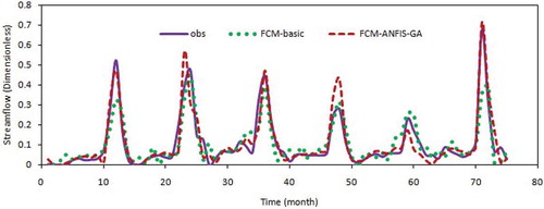
Figure 4. Comparison of the basic and GA based Sub-ANFIS model output for test period—Ajichai.

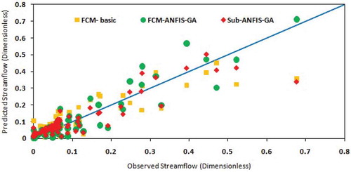
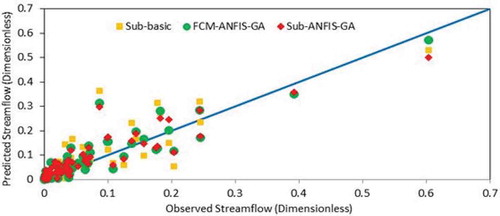
Figure 5. Comparison of scatter plots of different ANFIS models for test period—Lighvan.

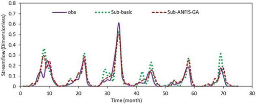
Figure 6. Comparison of scatter plots of different ANFIS models for test period—Ajichai.

4.2 GA input selection algorithm

As mentioned earlier, one of the main concerns about using a data-driven model is the selection of appropriate input variables. Using a large number of input variables or employing inappropriate datasets can lead to poor model performance especially during the test period. Redundant and irrelevant variables lead to a poor generalization performance, add error and noise to the model and prevent a correct learning process (May et al. 2011). In ANFIS, selecting the optimal subset of input variables can improve classification of inputs and production of fuzzy-based rules. In this study, a binary genetic algorithm was used for optimal input variable selection, as illustrated in Fig. 1. There are potentially 26 and 10 input variables of different kinds for the Ajichai and Lighvan basins, respectively (Table 4). These include lagged variables of precipitation, temperature and streamflow.

Table 4. Available data in Ajichai and Lighvan basins and optimal selection by GA*.

Basin	Data type
	Precipitation	Temperature	Discharge
Ajichai	Ghurigul	Sohzab	Vanyar
	Ghushchi	Mirkuh
	Nahand	Ghurigul
	Saeedabad
	Sarab
	Sbaghran
	Sohzab
	Vanyar
	Bostanabad
Lighvan**	Ghermezigul	Lighvan	Heravi
	Zinjenab
	Tabriz

*Optimal selections by GA in both basins are shown as bold and underlined.

** For Lighvan only lag 1 of data in all stations is selected.

The final results of input variable selection in Ajichai sub-basin indicate that, among the 26 variables shown in Table 4, precipitation for the previous month at Gushchi, Nahand and Sohzab stations and the previous month’s temperature at Mirkuh station plus the streamflow of the previous month at Vanyar have a greater ability to describe the current period streamflow at Vanyar station. Similarly, among the 10 variables shown in Table 4, the precipitation at Tabriz, Ghermezigul and Zinjenab stations, temperature at Lighvan and streamflow at Heravi, all from the previous month, are determined as the best variables for predicting the current period streamflow at Heravi station in the Lighvan Basin. Therefore, in Lighvan the number of inputs has been cut down by half (5 inputs) through excluding variables lagged by time step 2 (t – 2).

As shown in Tables 5 and 6, the optimal number of clusters in FCM-ANFIS—using GA input selection—and the optimal value of radius in Sub-ANFIS—using GA input selection—obtained by a sensitivity analysis are equal to 6 and 0.6, respectively, for Lighvan. For briefness, only the results for the Lighvan sub-basin have been shown in detail here. Using similar calculations for Ajichai, the optimum values of key parameters in FCM- and Sub-ANFIS models are presented in Table 2. According to Cobaner (2011), the proper values for radius should be within the interval of 0.2 and 0.5, but the optimum values in our application were determined to be slightly over this range. It should be noted that large radiuses produce few large clusters and a limited number of fuzzy rules. In contrast, a small number of clusters is due to a limited range of data points (of similar nature to data spaces). So, in this study, because of the limited range of data points, the higher radius was obtained. With the optimal values of parameters in hand, each model is evaluated and the results are presented in Table 3.

Table 5. Tuning of FCM-ANFIS-GA model for Lighvan.

Number of clusters	Train			Test
	R^2	RMSE	NSE	R^2	RMSE	NSE
6	0.86	0.050	0.86	0.86	0.053	0.85
7	0.81	0.056	0.81	0.81	0.057	0.81
8	0.84	0.054	0.84	0.83	0.053	0.83
9	0.83	0.054	0.83	0.83	0.054	0.81

Table 6. Tuning of Sub-ANFIS-GA model for Lighvan.

Radius	Train			Test
	R^2	RMSE	NSE	R^2	RMSE	NSE
0.55	0.81	0.057	0.81	0.80	0.060	0.79
0.6	0.81	0.057	0.81	0.81	0.058	0.80
0.65	0.77	0.063	0.77	0.77	0.063	0.77
0.7	0.80	0.060	0.80	0.79	0.061	0.78

It is evident from Table 3 that using optimal input variables selected by GA improves the results in comparison with those of the basic models in both basins. For FCM-ANFIS, the NSE indices for the Lighvan basin using basic and GA selected inputs (FCM-ANFIS-GA) are 0.74 and 0.85, respectively, showing 15% improvement, whereas for the Ajichai basin they are 0.66 and 0.82, indicating an improvement of 24%. In addition, the application of Sub-ANFIS using GA selected inputs (Sub-ANFIS-GA) shows 19% and 24% improvements in NSE values for the Lighvan and Ajichai basins, respectively. It can be seen from Table 3 that using the GA method to select inputs has slightly more effect on improving the results for Ajichai, being a large basin, than those for Lighvan, which is a small basin. This might be an indication that an optimal input selection algorithm would be more effective in large basins with too many variables than in small basins with limited variable choices.

A comparison of the results of GA-based models and basic models also shows that using more lagged precipitations is not necessary in this application. Therefore, in the remaining analysis, optimal inputs determined by the binary GA will be used in the hybrid WANFIS model.

Figures 3 – 6 show the time series and scatter plots of Sub- and FCM-ANFIS models for the test period of both basins. It is clear from these figures that using the GA selection method has had positive impact on the forecasting results. The solid line in the scatter plot shows where the perfect prediction occurs. Points above this line indicate overestimation, while those below the line show underestimation. Any trend in the predictions could be easily extracted from these plots. For briefness, only some selected results are shown in these graphs.

Figure 4 and Table 3 reveal that Sub- and FCM-ANFIS have almost similar performances in the Lighvan basin, but the highest peak flow was predicted more accurately by the FCM-ANFIS. Similarly, as can be seen from Fig. 6 and Table 3, Sub- and FCM-ANFIS present the same results and performance for the Ajichai basin. It is also clear that the differences between the two models are in classification of the input data and determining the initial rules. In this study, input data did not show significant sensitivity to the type of classification methods (FCM or subtractive clustering). Therefore, both models indicated almost a similar performance. It can be concluded that none of these methods was able to accurately catch the peak flows in either basin. Therefore the application of the wavelet transform method is investigated (Section 4.3) in order to improve the overall forecasting results.

4.3 Discrete wavelet transforms

A wavelet transform was applied on input data to further improve the performance of ANFIS models, especially on peak flows. Through wavelet decomposition, one approximate sub-signal of the original signal and several (equal to the number of decomposition stages) detailed sub-signals were obtained to explore hidden characteristics of the signal. In practice, a suitable level of decomposition is selected with respect to the nature of the time series. For instance, Kisi and Shiri (2011) applied three resolution levels to forecast daily precipitation in order to have variation and details of information on a nearly weekly scale (2³-day). Similarly, Nourani et al. (2011) used four decomposition levels for monthly time series forecasting, since a 2⁴-monthly scale represents the annual variation and details. However, the type of mother wavelet selection has rarely been discussed by researchers. The work by Nourani et al. (2011) is among the rare cases where sensitivity analysis is used to determine the best mother wavelet. Nevertheless, in most applications researchers use their own experience to choose a mother wavelet for their work (e.g. Wei et al. 2013).

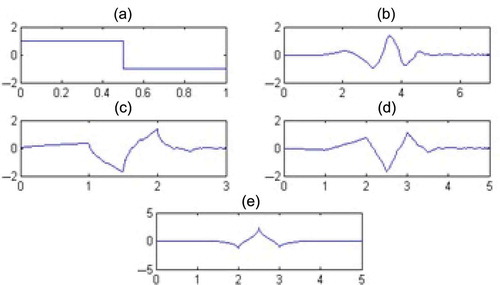
As shown in Fig. 7, the utilization of some mother wavelets, including Daubechises (db), sym, coif and Haar, was investigated in study. Among them, Haar is the simplest wavelet whereas db is the most widely used (Mallat 1998).

Figure 7. Mother wavelets: (a) Haar, (b) db4, (c) sym2, (d) sym3, (e) coif1.

As mentioned earlier, the optimal inputs determined by the binary GA are also used in wavelet-ANFIS (WANFIS) models. Here, for each mother wavelet, different decomposition levels have been tested. In the following sections, the results of applying wavelet-subtractive-ANFIS (Sub-WANFIS) and wavelet-FCM-ANFIS (FCM-WANFIS) in each study area are explained.

4.3.1 Sub-WANFIS

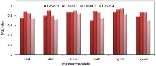
The general approach for selecting the best mother wavelet is the apparent similarity between mother wavelet and the time series. In this regard, Lighvan data have more similarities with sym2, sym3 and db4 wavelets. Figure 8 shows the results of investigating different types of mother wavelets and various levels of decomposition for the Lighvan basin. The results indicate that generally the sym2 mother wavelet has a higher NSE value and performs better than other wavelets for this basin.

Figure 8. Comparison of NSE values for different mother wavelets and decomposition levels using Sub-WANFIS for test period of Lighvan data.

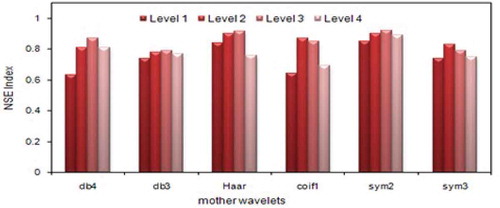
In addition, the resolution levels 1, 2, 3 and 4 have been applied for decomposing the signals. Once again, Fig. 8 shows that the model performance is best when three levels of decomposition are implemented. As can be seen, the model performance improved going from decomposition of level 1 to 2 and 2 to 3, while it is deteriorated when moving from decomposition of level 3 to level 4. Therefore, the sym2 mother wavelet with three decomposition levels is selected for Lighvan. Similar work was done for the Ajichai basin, where db4 with three decomposition levels was found suitable.

At this step, the Sub-WANFIS model is evaluated using the generated sub-signals. Table 7 shows a summary of the results, where the best value of radius and corresponding performance parameter values of the Sub-WANFIS model are presented. It is evident from Table 7 that all evaluation parameters are substantially improved using the wavelet method. For example, when the wavelet is applied using Sub-WANFIS, the best NSE value for the test period increased from 0.8 (Table 3) to 0.95 in (Table 7) for Lighvan. Similar improvements are observed for the Ajichai basin. Therefore, it is evident that the wavelet transformation has a significant positive role on streamflow prediction using the Sub-ANFIS model. In addition, similarly to the earlier approach, two basic models were defined using the same input variables as before to reveal the role of the input selection algorithm in wavelet models. It is evident from Table 7 that, similarly to regular ANFIS models, application of the input selection method (i.e. Sub-WANFIS-GA model) improves the results. For example, the NSE index of the Sub-WANFIS model for the Lighvan basin improved from 0.86 to 0.95 for the test period and from 0.91 to 0.97 for the training period when the input selection algorithm was used. Similar improvements were found for the Ajichai basin.

Table 7. Comparison of Sub-WANFIS models.

Basin	Radius	Method	Train			Test
			R^2	RMSE	NSE	R^2	RMSE	NSE
Lighvan	0.7	Basic-wave	0.91	0.04	0.91	0.87	0.048	0.86
	0.85	GA-wave	0.97	0.024	0.97	0.95	0.028	0.95
Ajichai	0.8	Basic-wave	0.94	0.035	0.93	0.85	0.061	0.85
	0.9	GA-wave	0.96	0.021	0.96	0.95	0.022	0.95

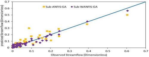
A comparison of streamflow hydrographs and scatter plots for Ajichai provided by (Figs 9 and 10) indicates the enhancements gained by using the wavelet transform. These findings support the values given in Table 7, showing that the accuracy of forecasts for peak streamflows is improved by using wavelet methods.

Figure 9. Comparison of Sub-ANFIS model output for the test period—Ajichai.

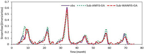
Figure 10. Comparison of scatter plots of Sub-ANFIS models for the test period—Ajichai.

4.3.2 FCM-WANFIS

A similar approach was followed to develop the FCM-WANFIS model. Six mother wavelets, including db4, db3, Haar, coif1, sym2 and sym3, were examined, among which sym2 was found to be the best wavelet for the Lighvan Basin (Fig. 11). Moreover, the resolutions of levels 1, 2, 3 and 4 were applied to decompose the main signal into several sub-signals and it was found that again three levels of decomposition had the best performance. Therefore, sym2 with three decomposition levels was used for the Lighvan data. Similarly, db4 with three decomposition levels was determined to be suitable for Ajichai. By decomposing signals to level 3 the performance was increased in both ANFIS models. The reason lies in the fact that the detailed sub-signal of decomposition level 3 represents 2³-scale, which approximately includes a seasonal scale consisting of 6 months. But, although the decomposition level 4 also includes 2³-scale, by decomposing signals to level 4 the results are not better than those in level 3. This is mainly due to an increase in the number of inputs, which leads to complexity of the model and thus reduction in the model performance.

Figure 11. Comparison of NSE values for different mother wavelets and decomposition levels using FCM-WANFIS for test period of Lighvan data.

The results of FCM-WANFIS are presented in Table 8 for both basins. Similarly to the Sub-WANFIS model, comparison of the results obtained by using the wavelet (Table 8) with those reached without using the wavelet (Table 3) reveals the significant role of wavelet decomposition on forecasted streamflow accuracy. Table 8 indicates that all evaluation criteria were substantially improved by the wavelet method. For example, when the wavelet was applied, the best NSE value for the test period for Lighvan data increased from 0.85 (Table 3) to 0.97 (Table 8).

Table 8. Results of FCM-WANFIS models.

Basin	No. of clusters	Method	Train			Test
			R^2	RMSE	NSE	R^2	RMSE	NSE
Lighvan	7	Basic-wave	0.93	0.036	0.92	0.88	0.042	0.88
	7	GA-wave	0.97	0.024	0.97	0.97	0.026	0.97
Ajichai	8	Basic-wave	0.92	0.031	0.92	0.86	0.060	0.85
	7	GA-wave	0.95	0.028	0.95	0.94	0.028	0.94

Comparison of streamflow hydrographs (Fig. 12) and scatter plots (Fig. 13) for Lighvan for the test period shows the superiority of the model using the wavelet, which supports the figures presented in Table 8.

Figure 12. Comparison of FCM-ANFIS models output for the test period—Lighvan.

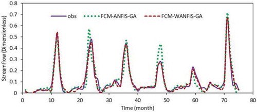
Figure 13. Comparison of scatter plots for FCM-ANFIS models for the test period—Lighvan.

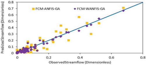
Moreover, the performances of FCM-WANFIS and Sub-WANFIS are very similar. These findings support those presented by previous researchers (Partal and Kisi 2007, Remesan et al. 2009, Shiri and Kisi 2010, Nourani et al. 2011, Calatao et al. 2011, Kalteh 2013). Table 9 shows a summary of all the results and reveals that the combination of the wavelet transform method and GA as data pre-processing methods can help to improve the forecasting significantly.

Table 9. Summary of comparison of models during test period.

Basin	Type of model	Model		Statistical parameter
				R^2	RMSE	NSE
Lighvan	Classic	Sub-ANFIS	Basic	0.70	0.076	0.67
			GA based	0.81	0.058	0.80
		FCM-ANFIS	Basic	0.74	0.068	0.74
			GA based	0.86	0.053	0.85
		Sub-WANFIS	Basic-wave	0.87	0.048	0.86
	Hybrid		GA-wave	0.95	0.028	0.95
		FCM-WANFIS	Basic-wave	0.88	0.042	0.88
			GA-wave	0.97	0.026	0.97
Ajichai	Classic	Sub-ANFIS	Basic	0.67	0.055	0.67
			GA based	0.83	0.045	0.83
		FCM-ANFIS	Basic	0.66	0.055	0.66
			GA based	0.82	0.047	0.82
		Sub-WANFIS	Basic-wave	0.85	0.061	0.85
	Hybrid		GA-wave	0.95	0.022	0.95
		FCM-WANFIS	Basic-wave	0.86	0.060	0.85
			GA-wave	0.94	0.028	0.94

5 Conclusions

The impact of using optimum input selection and wavelet transform was investigated on streamflow forecasting using an ANFIS model. The models were developed and evaluated using data from two different sized sub-basins of the Urmia Lake basin in northwestern Iran.

Input variable selection is a main concern in using data-driven models. The results showed that a significant improvement is gained through optimum selection of input variables for different ANFIS models in both basins. However, it was found that application of an optimum input selection algorithm is more important in large basins with many input variables as compared to small basins with limited choices. In addition, it was shown that using a wavelet transform in conjunction with the optimum input selection algorithm could substantially enhance the ANFIS performance: the improvements by the wavelet transform were found to be very significant in both basins. Moreover, there was no significant difference between the performance of Sub-ANFIS and FCM-ANFIS models in this application.

Disclosure statement

No potential conflict of interest was reported by the author(s).

References

- Adamowski, J. and Chan, H.F., 2011. A wavelet neural network conjunction model for groundwater level forecasting. Journal of Hydrology, 407, 28–40. doi:10.1016/j.jhydrol.2011.06.013
- Asadi, S., et al., 2013. A new hybrid artificial neural networks for rainfall–runoff process modeling. Neurocomputing, 121, 470–480. doi:10.1016/j.neucom.2013.05.023
- Bae, D.-H., Jeong, D.M., and Kim, G., 2007. Monthly dam inflow forecasts using weather forecasting information and neuro-fuzzy technique. Hydrological Sciences Journal, 52 (1), 99–113. doi:10.1623/hysj.52.1.99
- Bezdek, J., 1973. Cluster validity with fuzzy sets. Journal of Cybernetics, 3 (3), 58–73. doi:10.1080/01969727308546047
- Blum, A. and Langley, P., 1997. Selection of relevant features and examples in machine learning. Artificial Intelligence, 97, 245–271. doi:10.1016/S0004-3702(97)00063-5
- Bowden, G.J., Maier, H.R., and Dandy, G.C., 2005. Input determination for neural network models in water resources applications. Part 2. Case study: forecasting salinity in a river. Journal of Hydrology, 301, 93–107. doi:10.1016/j.jhydrol.2004.06.020
- Calatao, J.P.S., Pousinho, H.M.I., and Mendes, V.M.F., 2011. Hybrid wavelet-PSO-ANFIS approach for short-term wind power forecasting in Portugal. IEEE Transactions on Sustainable Energy, 2 (1), 50–59.
- Chang, F.-J. and Chang, Y.-T., 2006. Adaptive neuro-fuzzy inference system for prediction of water level in reservoir. Advances in Water Resources, 29 (1), 1–10. doi:10.1016/j.advwatres.2005.04.015
- Chiu, S., 1994. Fuzzy model identification based on cluster estimation. Journal of Intelligent and Fuzzy System, 2 (3), 267–278.
- Chiu, S., 1997. The fuzzy information engineering: a guided tour of applications. In: D. Dubois, H. Prade, and R. Yager, eds. Extracting fuzzy rules from data for function approximation and pattern classification. Springer: Berlin, 149–162.
- Cobaner, M., 2011. Evapotranspiration estimation by two different neuro-fuzzy inference systems. Journal of Hydrology, 398, 292–302. doi:10.1016/j.jhydrol.2010.12.030
- Dai, X., Wang, P., and Chou, J., 2003. Multiscale characteristics of the rainy season rainfall and interdecadal decaying of summer monsoon in North China. Chinese Science Bulletin, 48, 2730–2734. doi:10.1007/BF02901765
- Fernando, T.M.K.G., Maier, H.R., and Dandy, G.C., 2009. Selection of input variables for data-driven models: An average shifted histogram partial mutual information estimator approach. Journal of Hydrology, 367, 165–176. doi:10.1016/j.jhydrol.2008.10.019
- Grossman, A. and Morlet, J., 1984. Decomposition of Hardy functions into square integrable wavelets of constant shape. SIAM Journal on Mathematical Analysis, 15, 723–736. doi:10.1137/0515056
- Guyon, I. and Elisseeff, A., 2003. An introduction to variable and feature selection. The Journal of Machine Learning Research, 3, 1157–1182.
- Jang, J.-S.R., 1993. ANFIS: Adaptive-network-based fuzzy inference system. IEEE Transactions on System Man and Cybernetics, 23 (3), 665–685. doi:10.1109/21.256541
- Jeong, C., et al., 2012. Monthly precipitation forecasting with a neuro-fuzzy model. Water Resources Management, 26 (15), 4467–4483. doi:10.1007/s11269-012-0157-3
- Kalteh, A.M., 2013. Monthly river flow forecasting using artificial neural network and support vector regression models coupled with wavelet transform. Computers & Geosciences, 54, 1–8. doi:10.1016/j.cageo.2012.11.015
- Khazaee, P.R., Mozayani, N., and Motlagh, M.R.J., 2008. A genetic-based input variable selection algorithm using mutual information and wavelet network for time series prediction. IEEE Transactions on System Man and Cybernetics, 2133–2137.
- Kim, T.-W. and Valdés, J.B., 2003. Nonlinear model for drought forecasting based on a conjunction of wavelet transforms and neural networks. Journal of Hydrologic Engineering, 8 (6), 319–328. doi:10.1061/(ASCE)1084-0699(2003)8:6(319)
- Kişi, Ö., 2006. Daily pan evaporation modelling using a neuro-fuzzy computing technique. Journal of Hydrology, 329, 636–646. doi:10.1016/j.jhydrol.2006.03.015
- Kisi, O. and Shiri, J., 2011. Precipitation forecasting using wavelet-genetic programming and wavelet-neuro-fuzzy conjunction models. Water Resources Management, 25, 3135–3152. doi:10.1007/s11269-011-9849-3
- Kisi, O. and Shiri, J., 2012. Wavelet and neuro-fuzzy conjunction model for predicting water table depth fluctuations. Hydrology Research, 43 (3), 286–300.
- Kohavi, R. and John, G., 1997. Wrappers for feature subset selection. Artificial Intelligence, 97, 273–324. doi:10.1016/S0004-3702(97)00043-X
- Lefebvre, C.B., et al., 2000. Application of wavelet transform to hologram analysis: three-dimensional location of particles. Optics and Lasers in Engineering, 33, 409–421. doi:10.1016/S0143-8166(00)00050-6
- Mallat, S.G., 1998. A wavelet tour of signal processing. 2nd ed. San Diego: Academic Press.
- May, R., Dandy, G., and Maier, H., 2011. Review of input variable selection methods for artificial neural networks. In: K. Suzuki, ed. Artificial neural networks–methodological advances and biomedical applications. ISBN: 978-953-307-243-2, InTech, Available from: http://www.intechopen.com/books/artificialneural-networks-methodological-advances-and-biomedical-applications/review-of-input-variable-selectionmethods-for-artificial-neural-networks
- Moghaddamnia, A., et al., 2009. Evaporation estimation using artificial neural networks and adaptive neuro-fuzzy inference system techniques. Advances in Water Resources, 32, 88–97. doi:10.1016/j.advwatres.2008.10.005
- Nash, J.E. and Sutcliffe, J.V., 1970. River flow forecasting through conceptual models part I — A discussion of principles. Journal of Hydrology, 10 (3), 282–290. doi:10.1016/0022-1694(70)90255-6
- Nayak, P.C., et al., 2004. A neuro-fuzzy computing technique for modeling hydrological time series. Journal of Hydrology, 291, 52–66. doi:10.1016/j.jhydrol.2003.12.010
- Noori, R., et al., 2011. Assessment of input variables determination on the SVM model performance using PCA, Gamma test, and forward selection techniques for monthly stream flow prediction. Journal of Hydrology, 401, 177–189. doi:10.1016/j.jhydrol.2011.02.021
- Nourani, V., Kisi, Ö., and Komasi, M., 2011. Two hybrid Artificial Intelligence approaches for modeling rainfall–runoff process. Journal of Hydrology, 402, 41–59. doi:10.1016/j.jhydrol.2011.03.002
- Partal, T. and Kişi, Ö., 2007. Wavelet and neuro-fuzzy conjunction model for precipitation forecasting. Journal of Hydrology, 342, 199–212. doi:10.1016/j.jhydrol.2007.05.026
- Peng, Z.K. and Chu, F.L., 2004. Application of the wavelet transform in machine condition monitoring and fault diagnostics: a review with bibliography. Mechanical Systems and Signal Processing, 18, 199–221. doi:10.1016/S0888-3270(03)00075-X
- Rajaee, T., et al., 2011. River suspended sediment load prediction: application of ANN and wavelet conjunction model. Journal of Hydrologic Engineering, 16 (8), 613–627. doi:10.1061/(ASCE)HE.1943-5584.0000347
- Remesan, R., et al., 2009. Runoff prediction using an integrated hybrid modelling scheme. Journal of Hydrology, 372, 48–60. doi:10.1016/j.jhydrol.2009.03.034
- Sanikhani, H., et al., 2012. Estimation of daily pan evaporation using two different adaptive neuro-fuzzy computing techniques. Water Resources Management, 26 (15), 4347–4365. doi:10.1007/s11269-012-0148-4
- Santos, C.A.G. and Silva, G.B.L., 2014. Daily streamflow forecasting using a wavelet transform and artificial neural network hybrid models. Hydrological Sciences Journal, 59 (2), 312–324. doi:10.1080/02626667.2013.800944
- Sattari, M.T., Yurekli, K., and Pal, M., 2012. Performance evaluation of artificial neural network approaches in forecasting reservoir inflow. Applied Mathematical Modelling, 36 (6), 2649–2657. doi:10.1016/j.apm.2011.09.048
- Shiri, J. and Kisi, O., 2010. Short-term and long-term streamflow forecasting using a wavelet and neuro-fuzzy conjunction model. Journal of Hydrology, 394, 486–493. doi:10.1016/j.jhydrol.2010.10.008
- Szu, H., Telfer, B., and Garcia, J., 1996. Wavelet transforms and neural networks for compression and recognition. Neural Networks, 9, 695–708. doi:10.1016/0893-6080(95)00051-8
- Wang, W., et al., 2006. Forecasting daily streamflow using hybrid ANN models. Journal of Hydrology, 324, 383–399. doi:10.1016/j.jhydrol.2005.09.032
- Wei, S., et al., 2013. A wavelet-neural network hybrid modelling approach for estimating and predicting river monthly flows. Hydrological Sciences Journal, 58 (2), 374–389. doi:10.1080/02626667.2012.754102
- Yager, R.R. and Filev, D.P., 1994. Approximate clustering via the mountain method. IEEE Transactions on Systems Man and Cybernetics, 24 (8), 1279–1284. doi:10.1109/21.299710
- Zealand, C.M., Burn, D.H., and Simonovic, S.P., 1999. Short term streamflow forecasting using artificial neural networks. Journal of Hydrology, 214, 32–48. doi:10.1016/S0022-1694(98)00242-X
- Zhang, C. and Hu, H., 2005. Using PSO algorithm to evolve an optimum input subset for a SVM in time series forecasting. IEEE Transactions on Systems Man and Cybernetics, 4, 3793–3796.
- Zounemat-Kermani, M., 2013. Hydrometeorological parameters in prediction of soil temperature by means of artificial neural network: case study in Wyoming. Journal of Hydrologic Engineering, 18 (6), 707–718. doi:10.1061/(ASCE)HE.1943-5584.0000666