Geoinformatics in groundwater potential mapping and sustainable development: a case study from southern India

ABSTRACT

Groundwater potential in a basin is controlled by the amount of precipitation, nature of infiltration, lithology, geomorphology, soil and structure. Sustainable groundwater potential mapping emphasizes not only location of the potential groundwater zones, but also the optimum utilization of resources without affecting the aquifer systems. The Uppar Odai sub-basin in the Amaravati River basin, located in southern India, was selected for sustainable groundwater potential mapping through geoinformatics. In the present case, geomorphology, subsurface layer information derived from electrical resistivity data and lineaments were integrated for sustainable groundwater potential mapping. The structure contours indicate apparent resistivity zones at different depth configurations. The data were analysed at different depth perceptions of 25, 50, 75 and 100 m depth below ground level (b.g.l.). In order to assess the overall configuration of aquifer zones, profiles were plotted across the sub-basin in different directions. The geomorphology and lineaments interpreted from IRS P6 LISS III satellite data were integrated with resistivity data for the generation of a sustainable groundwater potential map. Ranking and weight were assigned for all thematic layers based on their importance in controlling the occurrence of groundwater. The spatial integration was carried out using ArcGIS 9.3 software. The integrated map shows three different potential zones as highly favourable, moderately favourable and least favourable groundwater potential zones. The results obtained through the GIS spatial integration are validated with water level data. Based on the present groundwater draft in the sub-basin, a sustainable groundwater plan is suggested.

Editor D. Koutsoyiannis Associate editor S. Grimaldi

KEYWORDS:

• GIS
• remote sensing
• geophysical methods
• geomorphology
• groundwater exploration
• sustainable development

Introduction

Geoinformatics is the appropriate platform for convergent analysis of diverse datasets for groundwater resource mapping and planning. Sustainable groundwater potential mapping involves the study of subsurface geological conditions, interpretation of landforms and of lineaments, where sustainable groundwater potential zones exist. Based on available resources, optimum groundwater development can be maintained in such zones. The demand for groundwater has increased due to increasing demographic pressure on its judicious utilization. Considering the depleting water resources and consequently the mounting problems, sustainable water resources development plans are needed (Nageswara Rao and Narendra 2006). In arid and semi-arid regions, groundwater plays a significant role in maintaining the sustainability of water resources (Chand et al. 2004). Under these circumstances, mapping of existing groundwater resources and forecasting the future resource-use scenarios are important. The integration of several parameters results in promising groundwater potential zones in a systematic way and forms an important aspect of groundwater studies. The groundwater potential map can show the quantitative conditions of groundwater, besides indicating probable sites for exploration. Geographical information systems (GIS) provide integrated information and knowledge from different data sources into the decision-making process and help in handling and management of large and complex databases. The GIS technique is not only useful in mapping groundwater potential zones through spatial integration but also provides the controlling terrain parameter. GIS and remote sensing tools are widely used for the management of various natural resources (Krishna Kumar et al. 2011, Magesh et al. 2011). In recent years, extensive use of satellite data along with conventional maps and ground truth data has made it easier to establish the base-line information for groundwater potential zones (Muralidhar et al. 2000, Chowdhury et al. 2010).

Remote sensing has become a vital tool for groundwater targeting, because the topographic expression and terrain characteristics have a direct relation to the characteristics of rocks and subsurface geological conditions. Integration of remote sensing data in the GIS environment is very useful in delineating various groundwater potential zones in a meaningful way (Agarwal et al. 2004). Many workers have adopted remote sensing and GIS techniques for groundwater exploration and identification of groundwater potential zones (Anbazhagan 1993, 1994, Chatterjee and Bhattacharya 1995, Teeuw 1995, Krishnamurthy et al. 1996, Saraf and Choudhury 1998, Goyal et al. 1999, Shahid and Nath 1999, Murthy 2000, OBI Reddy et al. 2000, Pratap et al. 2000, Anbazhagan et al. 2000, 2001, Sree Devi et al. 2001, Jaiswal et al. 2003, Anbazhagan 2004, Oseji et al. 2005, Narayanpethkar et al. 2006, Mondal et al. 2008, Sabale et al. 2009, Kumar et al. 2009, Kavitha et al. 2011). Researchers have also integrated GIS, remote sensing and geophysical data to derive thematic layers for groundwater potential mapping (Anbazhagan and Ramasamy 1997, Israil et al. 2006, Srivastava and Bhattacharya 2006, Ranganai and Ebinger 2008, Kumar et al. 2009). Geophysical methods can provide a better estimate of the depth and thickness of the aquifer system. Integration of surface hydrogeological features with subsurface information obtained from the geophysical survey provides reliable groundwater potential zones (Edet and Okereke 1997, Subba Rao and Prathap Reddy 1999, Shahid and Nath 2002). Oseji et al. (2005) have conducted a geophysical resistivity survey and integrated with borehole litholog data for aquifer characterization and groundwater potential mapping. Girish Kumar et al. (2010) have integrated electrical resistivity data with remote sensing outputs in a GIS environment for hydrogeological exploration. Geophysical resistivity data can be used for quantitative estimates of aquifer parameters (Dhakate and Singh 2005). Integrating geophysical resistivity data with other terrain parameters derived from high resolution satellite data provided more accurate information on groundwater potential zones in hard rock terrain (Rashid et al. 2012). Geophysical resistivity data were effectively utilized for generation of a Digital Basement Topographical Map (DBTM) to interpret aquifer storage estimation (Kumar et al. 2009).

Most of the integrated studies are restricted to groundwater potential mapping. Few studies are demonstrated with model validation. The objective of the present study is to demarcate potential groundwater zones along with a sustainable plan for further development. The resistivity data, geomorphology and lineaments were integrated for sustainable groundwater potential mapping. The resistivity layers at different depth configurations were studied so that the potential aquifers could be interpreted accurately. The study also considered the status of groundwater development, which is helpful for sustainable groundwater planning.

Study area

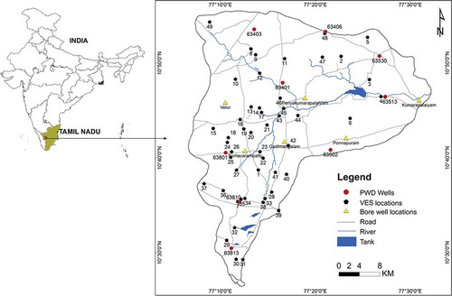
The Uppar Odai sub-basin is located in the Amaravati River basin in the state of Tamil Nadu, India, and falls between 77°6′36″E–77°32′24″E longitude and 10°26′40″N–10°55′48″N latitude. The aerial coverage of the Uppar Odai sub-basin is 1280 km². It covers the major part of Tiruppur district and a small area of Coimbatore district (Fig. 1). The annual average rainfall in the sub-basin is 625 mm, which is much lower than the state average rainfall (970 mm). A subtropical climate prevails throughout the region. The maximum temperature ranges from 27 to 35°C and minimum temperature varies from 17 to 23°C. There are four distinct seasons, namely southwest monsoon, northeast monsoon, winter season and hot weather period, prevailing in the study area. The rainfall pattern, as recorded at the rainfall stations, indicates that the precipitation is mostly uncertain, uneven or unequally distributed. It is slightly higher in the central and western parts and decreases in the northern and eastern parts of the sub-basin. The highest average annual rainfall of 738 mm is observed in the central part and the lowest amount of rainfall is 573 mm received in the northern part of the sub-basin.

Figure 1. Map showing the Uppar Odai sub-basin located in the western margin of Tamil Nadu State in southern India, with locations of vertical electrical soundings (VES), PWD observation wells and borewells.

Geology and hydrogeology

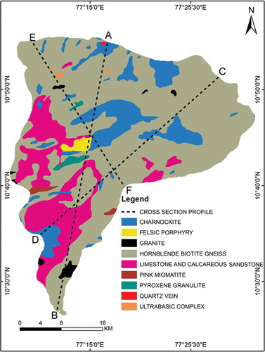
The southernmost part of the Indian Peninsula is a complex zone particularly characterized by rocks of granulite facies. The granulite terrain is composed not only of rocks of granulite facies, but amphibolite facies, gneisses and “supracrustal” rocks are also abundant, and some of these rocks are lower grade, representing areas of retrogression from granulite. The sub-basin area is underlined by a wide range of high grade metamorphic rocks of the Peninsular Gneissic Complex. The study area is composed solely of hornblende biotite gneiss, charnockites, pink migmatite, ultrabasic rocks, calc-silicate rocks, granites and pyroxene granulite (Viswanathan 1969, Narayanaswamy 1975) (Fig. 2). The rocks are extensively weathered and overlain by recent valley fills and alluvium in places. Groundwater occurs in almost all geological formations in the sub-basin at an average depth of 10 m below ground level (b.g.l.). During the pre-monsoon period (June to September) the water level reaches its deepest extent, to the maximum depth of 18 m b.g.l. Though such a water level decline is believed to be due to improper pumping and continuous demand, another important reason is essentially climatic factors, i.e. failure of the monsoon.

Figure 2. Geology of the Uppar Odai sub-basin, mostly covered by Precambrian crystalline rocks. The map also shows sections of geo-electrical resistivity profiles (AB: NNE–SSW, CD: NE–SW and EF: NW–SE).

Methodology

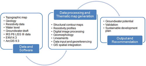
Survey of India topographic maps, a geology map published by GSI (1998), electrical resistivity data, satellite data, water level and data on groundwater draft were utilized in the present study. ArcGIS 9.3 software was utilized for data generation and spatial integration. The topographic maps were utilized for extraction of basin information such as roads and drainage. Electrical resistivity data were collected for 49 locations in the sub-basin from the Groundwater Department. The data were analysed for generation of a resistivity contour map at various depth perception and resistivity profiles. The electrical resistivity data include depth of sounding, apparent resistivity and location (latitude and longitude), which were entered into an Excel spreadsheet and converted into dbf format. The dbf files were imported to the GIS using the “add XY data” tool. The file was imported in the form of point data along with georeferences and then spatially interpolated using the inverse distance weighting (IDW) method.

The IRS P6 LISS III satellite data for the year 2012 were procured from the National Remote Sensing Centre (NRSC) and utilized for interpretation of geomorphology and lineaments. The pre-processed geometrically rectified satellite data were received in BIL format. The LISS III satellite data have four bands with 23.5 m spatial resolution. The satellite data were digitally processed with the help of ENVI 4.3 image processing software. The false colour composite (FCC), histogram equalization and pseudo-colour composite (PCC) images were generated for interpretation. The processed satellite outputs in raster format were imported to GIS using the “add data module”. The raster outputs used in the background, geomorphology and lineaments were interpreted and digitized by creating a “shape file”. All thematic maps were commonly projected to the “geographic coordinate system” with the WGS 1984 datum. Finally, structural contour maps derived from resistivity data, geomorphology and lineaments were integrated using the “weighted overlay analysis” method in GIS for groundwater potential mapping and sustainable development. The methodology adopted in the study is shown in Fig. 3.

Figure 3. Flow chart showing the methodology adopted in the study.

Electrical resistivity data analysis

Electrical resistivity data analysis is an important procedure adopted for groundwater potential mapping in this study. The vertical electrical soundings (VES) were spatially representative of the entire sub-basin. The maximum current electrode separation was 100 m. The resistivity vs current electrode separation for each location was plotted as graphs using RESIST Version 1.0 sounder software (Vander Velpen 1988). From those graphs, the thickness of the subsurface layers and their respective resistivity values were obtained.

Resistivity contour map

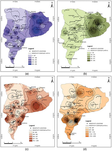
In the Wenner array, the separation between each electrode (a) is equal. The depth of investigation corresponds to the distance between the two electrodes. For example, if the distance between the two electrodes is 50 m, we get the result for depth of 50 m, and so on. Therefore, it is possible to present apparent resistivity contours for different electrode separations. In the present study, resistivity contour maps for 25, 50, 75 and 100 m b.g.l. were prepared. The interpretation of the resistivity soundings provides useful information on subsurface conditions. The soundings at selected stations provided resistivity variations with respect to depth and their correlation with the local geology. However, since 2D coverage of the soundings was spread over the entire area, it is possible to prepare maps of elevation contours of the subsurface interfaces of different layers obtained from resistivity soundings. These elevation contour maps, called structure contour maps (Twiss and Moores 1992), provide a qualitative regional correlation between the subsurface geology and the electrical resistivity. Structure contour maps were generated using resistivity maps at different depths for 25, 50, 75 and 100 m b.g.l. (Fig. 4). These maps show electrical resistivity values at particular depths in different locations in the sub-basin. For example, locations that show a low resistivity zone at a particular depth indicate that the aquifer zone extended to that particular depth. The low resistivity zones were separated out as favourable groundwater potential zones. The structural contour maps indicate favourable groundwater potential zones at different depths. The continuation of a low resistivity zone from one level to the next indicates the favourability condition for groundwater potential.

Figure 4. Structure contour for depth configurations of 25, 50, 75 and 100 m b.g.l. derived from electrical resistivity data.

Resistivity profiles and litho verification

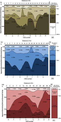
Geo-electrical resistivity profiles were drawn along different directions in the sub-basin (AB, CD and EF), which reflect the subsurface geological conditions (Fig. 2). The profile AB runs for 47 km and bisects the basin in the north–south direction (Fig. 5(a)). The depth sounding represents ≥100 m b.g.l. Overall the electrical resistivity profiles show four subsurface layer configurations: weathered, partially weathered, fractured and massive rock formations. This clearly depicts the thickness of aquifer zones across the sub-basin. The resistivity values range from 13 Ωm for the top layer to 862 Ωm for the bottommost layers. The profile shows maximum aquifer thickness in the middle, from 75 to 90 m depth b.g.l. In the southern part of the basin, the aquifer thickness is limited to the depth of 60 m b.g.l. The vertical section of borewell lithology was plotted for a well located at Somavarampatti village along this section, which shows that the aquifer thickness extends to 52 m b.g.l. The section CD runs from northeast to southwest, and passes through the central part of the sub-basin for about 42 km length (Fig. 5(b)). The central part of the basin is remarkably flat; on the western flank there are charnockites and the eastern part is covered by fractured charnockitic outcrops. The western and eastern regions are mostly associated with shallow aquifers and there are several productive dug wells present. A borewell (Vellore), located along this profile, shows the fractured formation extending to the depth of 60 m b.g.l. The section EF runs from northwest to southeast and passes through the central part of the sub-basin for 30 km (Fig. 5(c)). In the western part, calc silicate deposits are noticed along the stream channel, and on the eastern slope the felsic porphyry and fractured charnockites are exposed. In the eastern part, there are several productive dug wells located in the fractured charnockitic formation. The thickness of the aquifer zone extends to significant depth, to 75 m b.g.l. in the northwestern part and 100 m b.g.l. in the southeast zone. The available borewell (Gudimangalam) data show that the jointed charnockitic formation extends down to 40 m b.g.l. Out of these three resistivity profiles, the villages located along the northwest to southeast section show potential aquifer zones in the sub-basin. The borehole locations plotted along with resistivity profiles are shown in Fig. 5(c). The geo-electrical profiles and borewell litholog data show satisfactory correlation with a four-layer subsurface configuration at most of the locations. The general configuration represents soil, weathered, partially weathered and fractured formations. The litholog data obtained from borewells have shown that the middle fractured layer is underlain by massive formations.

Figure 5. Resistivity profile and borewell litholog along (a) AB, (b) CD and (c) EF sections.

Geomorphology

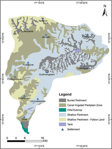
Geomorphology is one of the important parameters that control the movement and occurrence of groundwater in a sub-basin. In recent years, the increasing use of satellite data has made it easier to demarcate the spatial distribution of groundwater prospective zones on the basis of geomorphology (Sinha et al. 1990). Many researchers have effectively adopted geomorphology as the primary parameter in delineation of groundwater potential zones (Waters et al. 1990, Krishnamurthy et al. 1996, Singhal and Gupta 1999, Anbazhagan and Saranathan 2000, Sahu and Sahoo 2006). The various geomorphic units were interpreted using IRS P6 LISS III colour composite images as well as observations made in the field, such as topography, relief, aspect factor, soil and vegetative cover. Geomorphological investigations include the delineation and mapping of landforms and drainage characteristics that could have direct control on the occurrence of groundwater. The sub-basin area is covered by buried pediments, shallow pediments, shallow pediments associated with fallow land, canal-irrigated pediplain zones, hills/outcrop zones and tanks (Fig. 6). These land forms have different groundwater prospects in the sub-basin (Table 1). Buried pediments are found in the plains with varying thickness of weathered profile. Shallow pediments and canal-irrigated pediplain zones respectively occupy about 36% and 31% of the area in the sub-basin. These two geomorphic units control the major hydrological activities in the study area.

Table 1. Thematic layers, subsurface geology and associated groundwater prospects.

Thematic layers and units	Subsurface geological condition	Groundwater prospects	Aerial coverage (km^2)
Electrical resistivity
SC at 25 m depth with ≤250 Ωm zone	Soil, weathered and partially weathered formation	Favourable	1001
SC at 25 m depth with ≥250 Ωm zone	Less fractured, massive formation	Unfavourable	279
SC at 50 m depth with ≤250 Ωm zone	Fractured formation	Favourable	972
SC at 50 m depth with ≥250 Ωm zone	Massive formation	Unfavourable	308
SC at 75 m depth with ≤250 Ωm zone	Fractured formation	Favourable	279
SC at 75 m depth with ≥250 Ωm zone	Massive formation	Unfavourable	1001
SC at 100 m depth with ≤250 Ωm zone	Fractured, less fractured formation	Favourable	3
SC at 100 m depth with ≥250 Ωm zone	Massive, bedrock formation	Unfavourable	1277
Geomorphology
Buried pediment	Alluvial, colluvial and unconsolidated material; highly weathered formation, controlled by drainages and fractured zone	Good	163
Shallow pediments	Thin veneer of soil formation; partially weathered condition with occasional outcrops	Moderate	456
Shallow pediment with fallow land	Shallow pediment zone temporarily kept as barren land with moderate recharge condition	Moderate	164
Canal-irrigated pediplain zone	Canal irrigated, soil moisture zone with moderate recharge condition	Moderate	397
Hills/outcrops	Rocky outcrop zone with runoff condition	Poor	15
Tanks	Surface water storage and recharge zone	Good	85
Lineament density
High (55–125 km/km^2)	Highly fractured, jointed zone, good infiltration	Good	328
Moderate (20–55 km/km^2)	Moderately fractured zone with moderate recharge condition	Moderate	614
Low (0–20 km/km^2)	Limited weathered condition with limited infiltrations	Poor	338

SC: structure contour

Figure 6. Geomorphology of Uppar Odai sub-basin interpreted from IRS P6 LISS III satellite data.

Lineaments

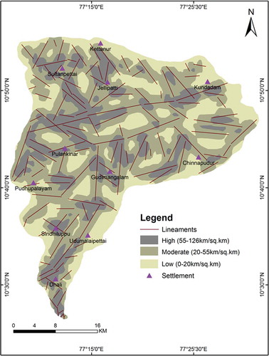
A lineament is defined as a significant line of landscape that reveals the hidden architecture of the rock basement (Hobbs 1904). It is essentially a simple or composite linear feature of a surface aligned in a rectilinear or slightly curvilinear relationship and which differs distinctly from the pattern of adjacent features and presumably reflects a subsurface phenomenon (O’Leary et al. 1976). Hence, lineaments are structural alignments, topographical expression, linear natural vegetation and lithological boundaries, etc., which are surface manifestations of buried structures (Gupta 2003). Lineaments are controlled by fractures, faults, joints and dykes, which are weak planes that act as conduits for movement and occurrence of groundwater. Gustafsson (1993) used GIS to analyse lineament data derived from SPOT imagery for groundwater potential mapping. Anbazhagan et al. (2001) interpreted lineaments from remotely sensed data and compared them with aquifer parameters. Lineaments in the sub-basin are of great importance in the present study as they are considered to be zones of good infiltration. The lineaments were identified using the tone, texture, relief, drainage and linear arrangement of vegetation in the satellite data. Lineaments and lineament intersection zones in the sub-basin enriched with vegetation cover were interpreted with the help of red tonal contrast in FCC and histogram equalized outputs. Linear drainage with moisture content was manifested as dark tonal contrast in the satellite data. Lineaments in the sub-basin are oriented in NNW–SSE, NE–SW, E–W and NW–SE directions. The lengths of the lineaments were measured in the calculation of the lineament density using the Density module in ArcGIS 9.3. The output image showed the lineament density at 1 km² area intervals. The lineament density was classified into high (55–126 km/km²), moderate (20–55 km/km²) and low (0–20 km/km²) density zones in the sub-basin (Fig. 7). The higher lineament density is directly related to favourable conditions for groundwater potential.

Figure 7. Lineament density map generated with the help of IRS P6 LISS III satellite data for Uppar Odai sub-basin.

Results and discussion

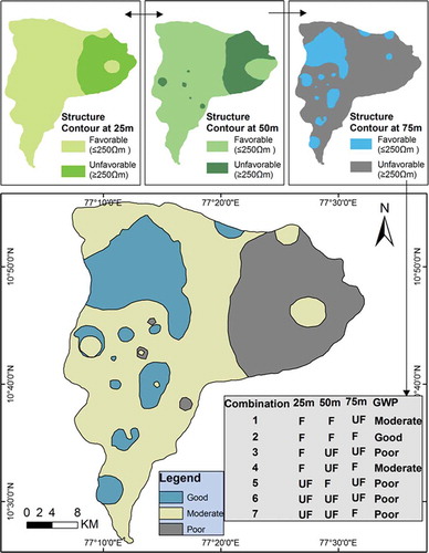
The thematic maps that reflect the subsurface geological conditions, including resistivity structure contour layers at different depth, geomorphology and lineaments, were considered for groundwater potential mapping. The potential zones in the sub-basin were delineated by integrating resistivity structure contours, geomorphology and lineaments in a GIS environment through weighted overlay methods available in the spatial analysis tool in ArcGIS 9.3 software. During the overlay analysis, the groundwater favourability condition was assessed for each individual thematic layer and the integrated output map was generated based on the combination of a number of favourable themes. The spatial integration was carried out at different stages by understanding each and every individual terrain parameter. Initially, the resistivity data were analysed at different depth configurations in the form of structure contour maps at 25, 50, 75 and 100 m b.g.l. Depending upon the resistivity value in the structure contours at various depths, we can understand the nature of weathered and fractured conditions at each location. The low resistivity zones invariably indicate weathered and fractured formations, where the probability of occurrence of groundwater is significant. If the low resistivity zones observed at all depths persist (25–100 m), then the area has favourable aquifer conditions and is considered as a good groundwater potential zone. Apparent resistivity greater than 250 Ωm in hard rock terrain normally represents the weathered and fractured zone, which is considered a favourable zone for groundwater occurrences. The low apparent resistivity value for the potential aquifer zone may vary slightly; in a practical sense it is difficult to place the boundary condition in real ground. In the present context, such low resistivity zones were buffered out at each layer stage (depth), as shown in Fig. 8. The low resistivity zones at different depths also indicate the available thickness of the aquifer zone and the possibility of good groundwater conditions (Table 1). Hence, at each stage the aquifer zone is classified into favourable and unfavourable (≤250 Ωm) groundwater potential zones. Again, the sub-basin area is divided into good, moderate and poor groundwater potential zones based on a combination of the number of favourable layers (Fig. 8). For example, a good groundwater potential zone in the sub-basin is a continuation of a low resistivity zone at maximum depth. In the sub-basin, it is very rare to observe low resistivity zones down to 100 m depth. Hence, a good groundwater potential zone extends at maximum to the third layer (75 m). In the case of a combination of any two low resistivity zones, it is classified as a moderate potential zone. Out of three layers, if any one layer supports the low resistivity condition, it is classified as of poor condition.

Figure 8. Layer stacking of low resistivity zones for different depth configurations (25, 50 and 75 m) and integrated groundwater potential zones for Uppar Odai sub-basin.

Based on recharge and subsurface geological conditions, the various landforms are classified into good, moderate and poor groundwater potential zones. The geomorphological units and respective groundwater prospecting zones are shown in Table 1. Among the various units, the buried pediments act as good groundwater prospective zones. The lineaments, interpreted from remote sensing data, act as good conduits for groundwater movement and accumulation. Based on the density of lineaments, the sub-basin area is categorized into high, moderate and low groundwater potential zones. The classified groundwater potential zones individually obtained for electrical resistivity, geomorphology and lineaments were separately integrated through GIS to get the final groundwater potential map. Before spatial integration, weights were assigned for each thematic layer (Table 2). Out of three thematic layers, more weight (40) is assigned to resistivity, since it gives a more realistic picture of subsurface conditions to the depth of 100 m b.g.l. Next, priority is given to lineament density, which favours good infiltration and groundwater movement. Geomorphology is assigned a weight of 25.

Table 2. Ranking and weight assignments of thematic layers for GIS spatial integration.

Thematic layer	Groundwater prospective zones	Rank	Weight	Score
Electrical resistivity	Good	10	40	400
	Moderate	8		320
	Poor	1		40
Geomorphology	Good	10	25	250
	Moderate	6		150
	Poor	1		25
Lineament density	High	10	35	350
	Moderate	6		210
	Low	2		70

Based on the importance of groundwater prospects, ranking was assigned for individual units in each thematic layer. For electrical resistivity, rankings of 10, 8 and 1 were assigned respectively for good, moderate and poor groundwater prospective zones. Similarly, rankings of 10, 6 and 1 were assigned for the levels of prospective zones in geomorphology. Lineaments carry rankings of 10, 6 and 2 respectively for high, moderate and low lineament density zones.

The thematic layers were separately integrated through the weighted overlay method available in ArcGIS 9.3 software. The integrated output map shows 19 zones (polygons) with a range of scores of 260–1000, which are controlled by combinations of three different thematic layers (Fig. 9). Based on the output score, the sub-basin is divided into highly favourable (752–1000), moderately favourable (506–752) and least favourable (260–506) groundwater potential zones (Fig. 10). The suitability of the ranking, weights and consistency can be assessed through consistency ratio and index calculation (Gupta and Srivastava 2010, Srivastava et al. 2012). In the present study such an assessment was not carried out and this is considered a limitation. In general, groundwater yield data are utilized to validate groundwater potential zones obtained through GIS spatial integration. However, the non-availability of pump test data in the sub-basin is the major constraint for utilizing yield data for validation. In the absence of yield data, water level data are used as an alternative.

Figure 9. Integrated groundwater potential mapping derived from weighted index overlay of resistivity, geomorphology and lineament density maps. The scores were obtained (shown in legend) through the spatially integrated value of ranking and weight assigned to the themes.

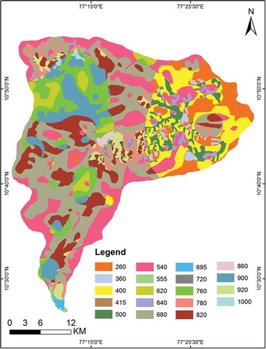
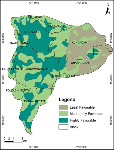
Figure 10. Sustainable groundwater potential zones in Uppar Odai sub-basin.

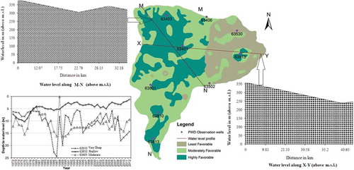
The integrated groundwater potential zone is validated through the water level data, which reflect the actual recharge condition and groundwater potential in a location. A comparative study has been carried out between the water level profile and groundwater potential zones obtained from GIS integrated analysis (Table 3). Water level data were collected from the Groundwater Department for the period 1972–2012. In order to understand the water table condition at various parts of the sub-basin, water table contours were drawn for two different sections MN and XY, respectively along the NW–SE and E–W directions (Fig. 11). The water table condition remains at more than 350 m a.m.s.l. along the NW–SE direction. It gradually decreases from west to east, indicating decline of the water table and the groundwater flow direction. Time series trends of groundwater level were drawn for three locations for 39 years. The results show that water level and groundwater potential match each other. The highly favourable groundwater potential zone coincides with shallow and moderate water level locations; the moderately favourable potential zone is associated with moderate water level conditions; and the poor groundwater potential zone mostly coincides with deep to very deep water level conditions (Fig. 11). For example, observation well 63513 shows very deep water level conditions in the sub-basin, and is located in the least favourable groundwater potential zone (Table 3).

Table 3. Observation wells with average water level in the sub-basin.

No.	Observation well	Average water level (m b.g.l.) (1972–2012)	Water level	Groundwater prospects zone
1	63401	9	Moderate	Moderately favourable
2	63403	9	Shallow	Highly favourable
3	63406	8	Moderate	Moderately favourable
4	63502	8	Moderate	Moderately favourable
5	63513	13	Very deep	Poor
6	63530	10	Moderate	Moderately favourable
7	63801	9	Shallow	Highly favourable
8	63810	7	Shallow	Highly favourable
9	63813	4	Shallow	Highly favourable

Table 4. Sustainable plan for groundwater potential zones in Uppar Odai sub-basin.

Stage	Block	a	b	c	Groundwater development category	Groundwater favourability condition	Sustainable groundwater planning
1	Gudimangalam	4965	4576	92	Critical zone	Block equally covered by high and moderately favourable groundwater condition	Currently under critical zone. Favourable groundwater condition supporting current status of groundwater development. However, water conservation measures are mandatory to sustain aquifer condition.
2	Madathukulam	6307	3560	56	Safe zone	Moderately favourable	Safe zone and favourable groundwater condition are in harmony with each other, so present level of groundwater extraction may continue.
3	Palladam	2745	2681	98	Critical zone	Moderately favourable	Currently under critical zone. Favourable groundwater condition supporting current status of groundwater development. However, water conservation measures are mandatory to sustain aquifer condition.
4	Pongalur	3636	2925	80	Semi-critical zone	Moderately to highly favourable	Though favourable groundwater conditions exist to some extent, groundwater draft reaches the semi-critical stage. Further increase of groundwater extraction should be restricted.
5	Udumalaipettai	9054	8581	91	Critical zone	Equally covered by highly and moderately favourable	Currently under critical zone. Favourable groundwater condition supporting current status of groundwater development. However, water conservation measures are mandatory to sustain aquifer condition.
6	Dharapuram	6800	4128	61	Safe zone	Least favourable	Least favourable groundwater conditions exist with safe level of extraction. Water-efficient cropping pattern recommended.
7	Kundadam	3836	2106	55	Safe zone	Least favourable	Least favourable groundwater conditions exist with safe level of extraction. Water-efficient cropping pattern recommended.
8	Sultanpet	3078	3294	107	Overexploited zone	Highly favourable	Present level of groundwater extraction is at alarming stage. Immediate attention is required to reduce the volume of groundwater extraction through water conservation practices and alternative cropping patterns.
9	Kinathukadavu	3750	3342	89	Critical zone	Equally covered by highly and moderately favourable	Currently under critical zone. Favourable groundwater condition supporting current status of groundwater development. However, water conservation measures are mandatory to sustain aquifer condition.
10	Pollachi north	4976	4652	93	Critical zone	Equally covered by highly and moderately favourable	Currently under critical zone. Favourable groundwater condition supporting current status of groundwater development. However, water conservation measures are mandatory to sustain aquifer condition.
11	Pollachi south	4932	4651	94	Critical zone	Moderately favourable	Currently under critical zone. Favourable groundwater condition supporting current status of groundwater development. However, water conservation measures are mandatory to sustain aquifer condition.

a: net groundwater availability (ha m), b: existing gross draft for all uses (ha m), c: status of groundwater development (%).

Figure 11. Model validation of groundwater potential zones through water level profile for different sections in the sub-basin. MN and XY respectively indicate the NW–SE and E–W directions.

The final groundwater potential zones were compared with the current level of groundwater draft to ascertain the sustainability condition of the aquifer (Table 4). The sub-basin area is covered by 11 administrative blocks (Fig. 10). Based on the percentage of groundwater development, the blocks can be categorized as overexploited (>100%), critical (90–100%), semi-critical (70–90%) and safe (<70%) zones (CGWB 2009). The data on groundwater draft were collected from the Central Ground Water Board (CGWB), and show the percentage of groundwater development in various blocks in the sub-basin. Comparing the present level of groundwater draft with the favourable groundwater potential condition, sustainable planning is derived for the sub-basin. The level of draft is at an “alarming” stage in eight blocks. The sustainable planning evolved for the sub-basin area is listed in the Table 4. For example, the overexploited blocks need immediate attention to reduce groundwater extraction through water construction practices and alternative farming patterns.

Conclusion

The integrated geophysical, remote sensing and GIS analyses provided practical output for groundwater potential mapping and sustainable planning. This is useful for further groundwater development, management practice and alternative cropping patterns. The structural contours derived from resistivity data show vertical as well as lateral distributions of favourable aquifer conditions for groundwater exploration. Geomorphology and lineaments, which are the surface manifestations of subsurface geology, interpreted from satellite data were also effectively utilized for demarcation of favourable groundwater potential zones in the sub-basin. The depth persistence of structural contours reveals that the aquifer condition extended to the maximum depth of 75 m b.g.l. The favourability condition for groundwater exploration very rarely exists at 100 m depth. Hence, installation of borewells beyond 75 m depth will not provide much yield to farmers. The knowledge-based ranking and weight assignment and weighted overlay analysis adapted in the GIS spatial integration provided a valuable output to demarcate the favourable groundwater potential zones. The high, moderate and least favourable groundwater potential zones in the basin respectively covered areas of 440, 570 and 270 km². Comparison of groundwater potential with water level and groundwater development data has shown appreciable correlation and validation of the results. The sustainable groundwater planning suggested will be useful for long-term groundwater development practice in the sub-basin.

Acknowledgements

The authors thank the Groundwater Department for providing resistivity and water level data. The groundwater draft data published from the CGWB report were utilized. The authors thank the anonymous reviewers for their valuable comments and suggestions to improve the content of the article.

Disclosure statement

No potential conflict of interest was reported by the authors.

Additional information

Funding

The second author acknowledges University Grants Commission (UGC), New Delhi, for granting an RGNF fellowship.

References

- Agarwal, A.K., Mohan, R., and Yadav, S.K.S., 2004. An integrated approach of remote sensing, GIS and geophysical techniques of hydrological studies in Rajpura block, Budaun district, Uttar Pradesh. Indian Journal of Power River Valley Development, 1, 35–40.
- Anbazhagan, S., 1993. Integrated Groundwater study in drought prone Pennagaram, Dharmapuri district, Tamil Nadu. Bulletin of the Indian Geologist Association, 26 (2), 117–123.
- Anbazhagan, S., 1994. Fracture pattern study for groundwater exploration in part of Dharmapuri district Tamil Nadu. Bhu-Jal News, 8 (2), 8–12.
- Anbazhagan, S., 2004. Geoinformatics for Hydrological studies. In: Proceedings of Regional Colloquium an Industry-Academia meet on advanced materials, Biosciences, and Computers and Information Technology, Daman, 25–27.
- Anbazhagan, S., Aschenbrenner, F., and Knoblich, K., 2001. Comparison of aquifer parameters with lineaments derived from remotely sensed data in kinzig basin. In: XXXI. IAH Congress: new approaches to characterizing groundwater flow. Germany, Munich, 2, 883–886.
- Anbazhagan, S. and Balamurugan, G., 2011. Remote sensing in delineating Deep Fractured Aquifer zones. In: S. Anbazhagan, S.K. Subramanian, and X. Yang, eds. Geoinformatics in applied geomorphology. New York, NY: CRC Press Taylor & Francis Group, 205–229.
- Anbazhagan, S. and Ramasamy, S.M., 1997. Geophysical resistivity survey and potential site selection for artificial recharge, India. In: P.G. Marinos, et al. ed. International symposium on engineering geology and environment. Athens, 2, 1169–1173.
- Anbazhagan, S. and Saranathan, E., 2000. Influence of geology, geomorphology and structure on groundwater condition in hard rock terrains of Tamil Nadu, India. In: Conference on groundwater exploration techniques, 30–31 March Tiruchirappalli, 1–6.
- Anbazhagan, S., Ramasamy, S.M., and Moses Edwin, J., 2000. Remote sensing and geophysical resistivity survey for groundwater exploration – a comparative analysis. In: Conference on groundwater exploration techniques, Tiruchirappalli. 177–181.
- Central Ground Water Board, 2009. report, 12–50.
- Chand, R., et al., 2004. Estimation of natural recharge and its dependency on subsurface geoelectric parameters. Journal of Hydrology, 299, 67–83. doi:10.1016/j.jhydrol.2004.04.001
- Chatterjee, R.S. and Bhattacharya, A.K., 1995. Delineation of the drainage pattern of a coal basin related inference using satellite remote sensing techniques. Asia Pacific Remote Sensing Journal, 1, 107–114.
- Chowdhury, A., Jha, M.K., and Chowdary, V.M., 2010. Delineation of groundwater recharge zones and identification of artificial recharge sites in West Medinipur district, West Bengal, using RS, GIS and MCDM techniques. Environmental Earth Sciences, 59, 1209–1222. doi:10.1007/s12665-009-0110-9
- Dhakate, R., and Singh, V.S., 2005. Estimation of hydraulic parameters from surface geophysical methods, Kaliapani ultramafic comple, Orissa, India. Journal of Environmental Hydrology, 13 (12), 1–11.
- Edet, A.E. and Okereke, C.S., 1997. Assessment of hydrogeological conditions in basement aquifers of the Precambrian Oban massif, southeastern Nigeria. Journal of Applied Geophysics, 36, 195–204. doi:10.1016/S0926-9851(96)00049-3
- Girish Kumar, M., Rameshwar Bali, and Agarwal, A.K., 2010. Integration of remote sensing and electrical sounding data for hydrogeological exploration-a case study of Bakhar watershed, India. The Hydrological Sciences Journal, 54 (5), 949–960.
- Goyal, S., Bharawadaj, R.S., and Jugran, D.K., 1999. Multicriteria analysis using GIS for groundwater resource evaluation in Rawasen and Pilli watershed, U.P. Available from: http://www.GISdevelopment.net.
- Gupta, M. and Srivastava, P.K., 2010. Integrating GIS and remote sensing for identification of groundwater potential zones in the hilly terrain of Pavagarh, Gujarat, India. Water International, 35 (2), 233–245. doi:10.1080/02508061003664419
- Gupta, R.P., 2003. Remote sensing geology. 2nd ed. Berlin Heidelberg: Springer.
- Gustafsson, P., 1993. High-resolution satellite imagery and GIS as a dynamic tool in groundwater exploration in a semi arid area. In: Application of geographic information systems in hydrology and water resources management (Proc.HydroGIS Conf., Vienna, Austria, April 1993) (ed. by K. Kovar and H.P. Nachtnebel), 93–100. IAHS Publ. 211, IAHS Press, Wallingford, UK. Available from: http://iahs.info/redbooks/b211/211011.pdf.
- Hobbs, W.H., 1904. Lineaments of the Atlantic border region. Geological Society of American Bulletin, 15, 483–506.
- Israil, M., et al., 2006. Groundwater resources evaluation in the Piedmont zone of Himalaya, India, using isotope and GIS technique. Journal Spatial Hydrology, 6 (1), 34–38.
- Jaiswal, R.K., et al., 2003. Role of remote sensing and GIS techniques for generation of groundwater prospect zones towards rural development-an approach. International Journal of Remote Sensing, 24, 993–1008. doi:10.1080/01431160210144543
- Kavitha, M., Mohana, P., and Naidu, K.B., 2011. Delineating groundwater potential zones in Thurinjapuram watershed using geospatial techniques. Indian Journal of Science and Technology, 4 (11), 1470–1476.
- Krishna Kumar, S., et al., 2011. Hydrogeochemical study of shallow carbonate aquifers, Rameswaram Island, India. Environmental Monitoring and Assessment. Available from: http://dx.doi.org/10.1007/s10661-011-2249-6
- Krishnamurthy, J., et al., 1996. Influence of rock types and structures in the development of drainage networks in typical hard rock terrain. ITC Journal, 3 (4), 252–259.
- Kumar, A., Savita, T., and Prasad, L.B., 2009. Groundwater prospects analysis through hydrogeophysical parameters and hydrogeomorphic zonation - a case study in parts of Kewta Watershed, upper Barakar basin, Bihar. Available from: GISdevelopment.net.
- Kumar, J.R., Balasubramanian, T.A., and Kumar, A., 2011. Delineation and evaluation of groundwater potential zones using electrical resistivity survey and aquifer performance test in Uppodai of Chittar – Uppodai water shed, Tambaraparani River Basin, Tirunelveli-Thoothukudi Districts, Tamilnadu. Journal of Indian Geophysical Union, 15 (2), 85–94.
- Magesh, N.S., Chandrasekar, N., and Soundranayagam, J.P., 2011. Morphometric evaluation of Papanasam and Manimuthar watersheds, parts of Western Ghats, Tirunelveli district, Tamil Nadu, India: a GIS approach. Environmental Earth Sciences, 64, 373–381. doi:10.1007/s12665-010-0860-4
- Mondal, N.C., Das, S.N., and Singh, V.S., 2008. Integrated approach for identification of potential groundwater zones in Seethanagaram Mandal of Vizianagaram District, Andhra Pradesh, India. Journal of Earth System Science, 117 (2), 133–144. doi:10.1007/s12040-008-0004-3
- Muralidhar, M., et al., 2000. Remote sensing applications for the evaluation of water resources in rainfed area, Warangal district, Andhra Pradesh. The Indian Mineralogists, 34, 33–40.
- Murthy, K.S.R., 2000. Ground water potential in a semi-arid region of Andhra Pradesh - a geographical information system approach. International Journal of Remote Sensing, 21 (9), 1867–1884. doi:10.1080/014311600209788
- Nageswara Rao, K. and Narendra, K., 2006. Mapping and evaluation of urban sprawling in the Mehadrigedda watershed in Visakhapatnam metropolitan region using remote sensing and GIS. Current Science, 91, 1552–1557.
- Narayanaswamy, S., 1975. Proposal for charnockite-khondalite system in the Archean shield of Peninsular India. Geological Survey of India, Mise. Publ., 23 (1), 1–16.
- Narayanpethkar, A.B., Vasanthi, A., and Mallick, K., 2006. Electrical resistivity technique for exploration and studies on flow pattern of groundwater in multi-aquifer system in the basaltic terrain of the Adila basin, Maharashtra. Journal of the Geological Society of India, 67 (1), 69–82.
- O’leary, D.W., Friedman, J.D., and Pohn, H.A., 1976. Lineament, linear and lineation: some proposed new standards for old terms. Geological Society of America Bulletin, 87, 1463–1469. doi:10.1130/0016-7606(1976)87<1463:LLLSPN>2.0.CO;2
- OBI Reddy, G., et al., 2000. Evaluation of groundwater potential zones using remote sensing data—a case study of Gaimukh watershed, Bhandaradistrict, Maharashtra. Journal of the Indian Society of Remote Sensing, 28 (1), 19–32. doi:10.1007/BF02991858
- Oseji, J.O., Atakpo, E.A., and Okolie, E.C., 2005. Geoelectric investigation of the aquifer characteristics and groundwater potential in Kwale, Delta state, Nigeria. Journal of Applied Science Environmental Management, 9 (1), 157–160.
- Pratap, K., Ravindran, K.V., and Prabakaran, B., 2000. Groundwater prospect zoning using remote sensing and geographical information system: a case study in Dala-Renukoot area, Sonbhadra district, Uttar Pradesh. Journal of the Indian Society of Remote Sensing, 28, 249–263. doi:10.1007/BF02990815
- Ranganai, R.T. and Ebinger, C.J., 2008. Aeromagnetic and landsat TM structural interpretation for identifying regional groundwater exploration targets, south-central Zimbabwe Craton. Journal of Applied Geophysics, 65, 73–83. doi:10.1016/j.jappgeo.2008.05.009
- Rashid, M., Lone, M., and Ahmed, S., 2012. Integrating geospatial and ground geophysical information as guidelines for groundwater potential zones in hard rock terrains of south India. Environmental Monitoring and Assessment, 184, 4829–4839. doi:10.1007/s10661-011-2305-2
- Sabale, S.M., Ghodake, V.R., and Narayanpethkar, A.B., 2009. Electrical resistivity distribution studies for artificial recharge of groundwater in the Dhubdhubi Basin, Solapur District, Maharashtra, India. Journal of Indian Geophysical Union, 13 (4), 201–207.
- Sahu, P.C. and Sahoo, H., 2006. Targeting ground water in tribal dominated Bonai area of drought-prone Sundargarh District, Orissa, India—a combined geophysical and remote sensing approach. Journal of Human Ecology, 20 (2), 109–115.
- Saraf, A.K. and Choudhury, P.R., 1998. Integrated remote sensing and GIS for ground water exploration and identification of artificial recharge sites. International Journal of Remote Sensing, 19 (10), 1825–1841. doi:10.1080/014311698215018
- Shahid, S. and Nath, S.K., 1999. GIS integration of remote sensing and electrical sounding data for hydrogeological exploration. Journal of Spatial Hydrology, 2 (1), 1–12.
- Shahid, S., and Nath, S.K., 2002. GIS integration of remote sensing and electrical sounding data for hydrogeological exploration. Journal of Spatial Hydrology, 2 (1), 1–12.
- Singhal, B.B.S. and Gupta, R.P., 1999. Applied hydrogeology of fractured rocks. India: Department of Earth Sciences University of Rookee.
- Sinha, B.K., et al., 1990. Integrated approach for demarcating the fracture zone for well site location : a case study near Gumla and Lohardaga, Bihar. Journal of the Indian Society of Remote Sensing, 18 (3), 1–8. doi:10.1007/BF03030727
- Sree Devi, S., Srinivasulu, S., and Raju, K.K., 2001. Delineation of groundwater potential zones and electrical resistivity studies for groundwater exploration. Environmental Geology, 40 (10), 1252–1264. doi:10.1007/s002540100304
- Srivastava, P.K. and Bhattacharya, A.K., 2006. Groundwater assessment through an integrated approach using remote sensing, GIS and resistivity techniques: a case study from a hard rock terrain. International Journal of Remote Sensing, 27 (20), 4599–4620. doi:10.1080/01431160600554983
- Srivastava, P.K., et al., 2012. Integrated framework for monitoring groundwater pollution using a geographical information system and multivariate analysis. Hydrological Sciences Journal, 57 (7), 1453–1472. doi:10.1080/02626667.2012.716156
- Subba Rao, N. and Prathap Reddy, R., 1999. Groundwater prospects in a developing satellite township of Andhra Pradesh, India using remote sensing techniques. Journal of the Indian Society of Remote Sensing, 27 (4), 193–203. doi:10.1007/BF02990832
- Teeuw, R.M., 1995. Groundwater exploration using remote sensing and a low-cost geographical information system. Hydrogeology Journal, 3 (3), 21–30. doi:10.1007/s100400050057
- Twiss, R.J. and Moores, E.M., 1992. Structural geology. New York, NY: W.H. Freeman and Company.
- Vander Velpen, B.P.A., 1988. Resist Version 1.0. Delf Netherland: MSc Research Project, ITC.
- Viswanathan, T.V., 1969. The granulite rocks of the Indian Precambrian Shield. Geological Survey of India, 100, 37–66.
- Waters, P., et al., 1990. Applications of remote sensing to groundwater hydrology. Remote Sensing Reviews, 4 (2), 223–264. doi:10.1080/02757259009532107