Regionalisation of hydrological responses under land-use change and variable data quality

ABSTRACT

Estimating river flows at ungauged sites is generally recognised as an important area of research. In countries or regions with rapid land development and sparse hydrological gauging networks, three particular challenges may arise—data scarcity, data quality, and hydrological non-stationarity. Using data from 44 gauged sub-catchments of the upper Ping catchment in northern Thailand from the period 1995–2006, three relevant flow response indices (runoff coefficient, base flow index and seasonal elasticity of flow) were regionalised by regression against available catchment properties. The runoff coefficient was the most successfully regionalised, followed by base flow index and lastly the seasonal elasticity. The non-stationarity (represented by the differences between two 6-year sub-periods) was significant both in the flow response indices and in land use indices; however relationships between the two sets of indices were weak. The regression equations derived from regionalisation were not helpful in predicting the non-stationarity in the flow indices except somewhat for the runoff coefficient. A partly subjective data quality scoring system was devised, and showed the clear influence of rainfall and flow data quality on regionalisation uncertainty. Recommendations towards improving data support for hydrological regionalisation in Thailand include more relevant soils databases, improved records of abstractions and investment in the gauge network. Widening of the regionalisation beyond the upper Ping and renewed efforts at using remotely sensed rainfall data are other possible ways forward.

EDITOR Z.W. Kundzewicz ASSOCIATE EDITOR T. Wagener

KEYWORDS:

• predictions in ungauged basins
• rainfall–runoff indices
• signatures
• data quality
• land-use change
• Thailand
• Ping basin

1 Introduction

River flow data are known to be important for a variety of water resources and flood management applications. Flow data can be obtained easily in catchments with networks of flow gauges and if necessary the record can be extended by using a locally calibrated rainfall–runoff model. However, many catchments remain ungauged or poorly gauged, for example because of lack of budget for installing and maintaining gauging equipment, and environmental constraints on locations of gauges. Methods of modelling flows in ungauged catchments, where local calibration of rainfall–runoff models is not an option, are therefore needed. Much research on this topic has been done using spatial generalisation, or regionalisation, techniques (Croke et al. 2004, Wagener et al. 2004, McIntyre et al. 2005, Young 2006, Boughton and Chiew 2007, Yadav et al. 2007, Oudin et al. 2008b, Li et al. 2009, Bulygina et al. 2012, Gibbs et al. 2012). Usually, one of three general regionalisation approaches is used: transfer of information about flow responses from the closest gauged catchment (or pool of catchments) to the catchment of interest; transfer from a physically similar gauged catchment (or pool of catchments); or regression of flow responses against measured catchment properties. The information about flow responses may either be in the form of rainfall–runoff model parameters, or in the form of relevant flow indices such as the runoff coefficient (Nathan and McMahon 1992, Burn and Boorman 1993, Sefton and Howarth 1998, Croke and Norton 2004, Merz and Blöschl 2004, Yadav et al. 2007, Zhang and Chiew 2009). Each method has strengths and weaknesses, and performance is variable depending on, for example, catchment topography, climate condition, and quality of hydrological data and number of gauged catchments (Bao et al. 2012).

Almost all of the published regionalisation studies, such as those cited above, use case studies in relatively well-gauged and well-developed countries. Other countries suffer from more limited hydrological and catchment properties (e.g. soils) data, and greater data quality problems that may affect the approach taken (Hughes et al. 2006b, Winsemius et al. 2009, Kapangaziwiri et al. 2012, Sikorska et al. 2012). Furthermore, in some areas, the observed hydrological responses are affected by rapid land use change or other sources of hydrological non-stationarity that may complicate the spatial generalisation (e.g. Bari et al. 1996, Chiew et al. 2009, McIntyre and Marshall 2010, Peel and Blöschl 2011). These particular challenges—regionalisation using more limited data sets and under non-stationary conditions—have not been addressed extensively in the literature. It has also been suggested that signals in the relationship between hydrological response and land use, which have been derived through empirical spatial analysis, can be used to predict the impacts of temporal changes in land use as an alternative or complement to physics-based hydrological modelling (Wagener 2007, Singh et al. 2011, Bulygina et al. 2012, McIntyre et al. 2014). If this “trading space for time” approach can be shown to be applicable then it may be an especially useful tool for water resource planning in regions that are subject to rapid land use change.

Managing data and model uncertainty is an important component of evaluating suitability of regionalisation schemes for prediction in ungauged catchments. Uncertainty is present in input climate data, observed flow, and also arises from simplification of the real-world processes in modelling and in the regionalisation scheme (Wagener et al. 2004, Hughes et al. 2006b, Kjeldsen and Jones 2010, Hrachowitz et al. 2013). Analysing the effects of these sources of uncertainty on quality of model outputs can improve understanding of priorities for data collection and model improvement, and can avoid over-confidence in decisions that are based on the model predictions or wrong inferences about factors affecting the hydrological response (Brown and Heuvelink 2006, Hughes et al. 2010). Using uncertainty analysis also provides a framework through which the value of different regionalisation approaches can be assessed, with the better methods giving more accurate and more precise outputs (Bulygina et al. 2011).

This paper addresses some of the issues that arise when predicting flows in ungauged catchments under data scarcity, variable data quality and hydrological non-stationarity using a case study of 44 gauged sub-catchments of the mountainous upper Ping catchment in northwest Thailand. The objectives are: (1) to assess the applicability of using regression for regionalisation of flow indices; (2) to investigate links between data quality and regression performance by plotting a data quality metric against a performance metric; (3) to evaluate the effects of deforestation on the uncertainty in the regional regression; (4) to evaluate the ability of that regression to predict the effects of deforestation on flows by plotting observed versus predicted indices; and hence (5) to make some specific recommendations about improving flow predictions in the case study catchments and in comparable regions.

While alternative approaches to regionalisation that aim to transfer information about flow response from clusters of similar catchments (McIntyre et al. 2005, Reichl et al. 2009, Kumar et al. 2013) might be used instead of regression, the regression approach is adopted because: it estimates an explicit link between the flow response and the catchment properties and so may add to understanding of dominant mechanisms; an estimate of the error variance is an output of the regression analysis allowing uncertainty analysis; and numerous studies have shown the regression method to be useful for making predictions in ungauged catchments when using a comparable number of gauged catchments (Sefton and Boorman 1997, Fernandez et al. 2000, Mazvimavi et al. 2005, Heuvelmans et al. 2006, Pallard et al. 2009).

2 Description of the upper Ping catchment

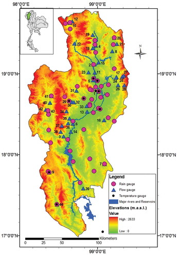
The upper Ping catchment, with an approximate area of 25 370 km², is situated in the northwest of Thailand, as shown in Fig. 1. North of the catchment is Myanmar, west of the catchment is the Salawin catchment, and the Kok and Wang catchments are to the northeast and southeast, respectively. The Ping catchment is the largest catchment contributing to the Chao Phraya River catchment (Thanapakpawin et al. 2007), in which Bangkok is located. The improved planning and design that may be permitted by better methods of flow estimation would be beneficial to many communities and businesses in the Chao Phraya River catchment at risk from floods or droughts.

Figure 1. Location plan with elevations and locations of hydrological gauges.

2.1 Topography and soils

The elevations range from mean sea level to 2633 metres above mean sea level (m a.s.l.), with the central alluvial plains being surrounded by mountains (Fig. 1). Out of 44 sub-catchments, 42 used in this study have mean slopes of more than 20%, and are considered here to be “steep” catchments. “Mountainous soil” is the most prevalent soil type covering 69% of the upper Ping catchment (Land Development Department 2006). This soil type, commonly found where the slope is greater than 35%, is associated with weathered rocks, which range from the oldest Precambrian to the latest Igneous (Wongprayoon and Saengsrichan 2004, Department of Mineral Resources 2010); however, no estimates of soil hydrological properties are available. Soil depth is variable and is subject to high erosion, although deep and more stable soil layers can be found under dense forests. Sandy loam with fragmented rock and clay can be found widely in some areas of the basin where the slope is less than 35%. Other soil types cover only small, localised areas.

2.2 Land use

The major land use is forest including dry dipterocarp, mixed deciduous, dry evergreen, hill evergreen and coniferous forests. The dry dipterocarp and mixed deciduous forests, consisting of teak, Afzelia xylocarpa, Pterocarpus macrocarpus, rosewood and Xylia xylocarpa Taub (leguminosae), are found in the valleys and hills at elevations less than 1000 m a.s.l., while the evergreen and coniferous are common at higher elevations. The principal commercial crops grown are rice, corn, longan and other tropical fruit trees. Agriculture is common to the alluvial plains along both sides of the upper Ping River. The major land-use change from 1995 to 2006 was deforestation and conversion to crops and pastoral agriculture areas. The degree of urban cover is low, ranging from zero to 5% of the gauged sub-catchment areas.

2.3 Climate and hydrology

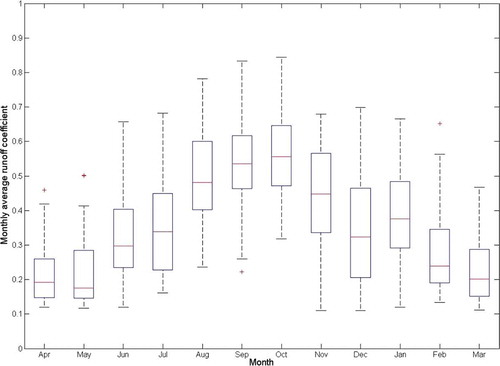
Figure 2 shows the annual rainfall pattern for 50 rain gauges over the upper Ping, illustrating that there are three seasons, commonly called the rainy, winter and summer seasons. The rainy season is between mid-May and mid-October (the Southwest monsoon), while winter is between mid-October and mid-February (the Northeast monsoon). Summer, from mid-February to mid-May, is usually dry and hot. The first peak of rainfall in May is caused by the arrival of the Inter-Tropical Convergence Zone (ITCZ). The rapid movement of the ITCZ from the south to the north of the basin and into the south of China between June and July triggers a period of rainfall deficit that can lead to drought. In August, the ITCZ moves back from the south of China to the north of Thailand causing a second, longer period of high rainfall (Fig. 2). The peaks of rainfall are more pronounced if tropical cyclones are present. In October, rainfall decreases because the Northeast monsoon brings cold dry air from the anticyclone in mainland China. This is followed by several months of low rainfall, prior to the return of the Southwest monsoon, that make March and April prone to drought. Figure 3 shows the ratio of long-term runoff to long-term rainfall (the runoff coefficient) for the 44 flow gauges used in this study, showing that runoff coefficients are highly variable in space and in time. This spatial variation in runoff coefficient may be due to differences in topography, land use and soil type (this will be explored further in the results section below), while the temporal variation, peaking in October after the rainy season, is explained by the antecedent wetness.

Figure 2. Box plot showing monthly average rainfall statistics for the 50 rain gauges.

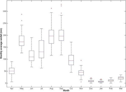
Figure 3. Box plot showing monthly runoff coefficient statistics for the 44 flow gauges.

There are three reservoirs in the upper Ping catchment. The Mae Ngud Somboon Chon and Mae Kuang Udomthara reservoirs have effective storages of 243 × 10⁶ m³ and 249 × 10⁶ m³, respectively (WMSC (Water Watch and Monitoring System for Warning Center) 2010). They were built for agricultural supply and flood and drought relief (Royal Irrigation Department 2003). No clearly contradictory flow responses were seen at the gauges below these reservoirs so it is assumed that they are sufficiently small that they do not affect the downstream flow regime enough to disqualify them from this analysis. Located at the low end of the upper Ping catchment is the Bhumibol Dam, with an effective storage of 9662 × 10⁶ m³ (WMSC 2010). The flow gauges downstream of this dam were excluded from the analysis. Electric and diesel pumping stations operated by government agencies are found throughout the basin, strictly regulated by a water users’ group committee. These abstractions could affect flows; however, no data on abstraction volumes are available.

2.4 Hydrological and climate data

Rainfall and temperature data used in this study were obtained from three sources: the Thai Meteorological Department (TMD), the Royal Irrigation Department (RID) and the Department of Water Resources (DWR). Flow data were provided by the RID and the DWR. This study uses daily data from 50 rain gauges and 10 temperature gauges across 44 sub-catchments, each of which has a flow gauge at its outlet. The locations of gauges are shown in Fig. 1. The water years (April to March) from 1995 to 2006 were chosen for this study because they provided a long enough period to assess model performance and recent land use change, and had relatively complete records for the available flow and rain gauges.

Apart from ground observations of rainfall, various satellite products were considered. However, previous analysis (Visessri and McIntyre 2012) showed that the spatial rainfall estimation provided by the TRMM 3B42 V6 satellite product produced estimates of a similar accuracy to those provided by a customised technique for interpolating between ground gauges based on inverse distance weighting with an elevation adjustment, and hence only the latter rainfall estimation method was used here.

3 Methods description

3.1 Choice of flow indices

Three flow indices were estimated for each gauged sub-catchment: the runoff coefficient (RC), the base flow index (BFI) and the rainfall–flow seasonal elasticity (EL). The analysis could easily be extended to include more indices; however, for water resources planning, RC, BFI and EL are considered to be key indices, together representing flow volumes and flow distribution from the daily to the seasonal scales. Furthermore, especially in data-sparse regions, it is likely that little further information about flow response may be gained when using more than three regionalised indices (Yadav et al. 2007, Zhang et al. 2008, Kapangaziwiri et al. 2009, Almeida et al. 2012). Table 1 shows that there is some dependency between the chosen three indices, which should be accounted for when applying their modelled values (Almeida et al. 2012).

Table 1. Matrix of scatter plots and correlation coefficients (r) between the sub-catchment properties and the three flow indices (RC, BFI and EL). r values that are significant at the 95% level are shown in bold. Abbreviated sub-catchment properties are defined in Section 3.2.

Variable	A	ELE	SLP	CHL	DD	%MS	%AGR	%FOR	%MIX	%URB	%WAT	MAR	MWR	MDR	RC	BFI	EL
A	1	−0.36	−0.17	1.00	−0.09	−0.29	0.26	−0.35	0.29	0.43	0.79	0.05	−0.04	0.01	−0.32	−0.16	0.21
ELE		1	0.51	−0.35	0.15	0.62	−0.06	0.14	−0.32	−0.29	−0.47	0.15	0.29	0.00	0.67	0.59	−0.39
SLP			1	−0.17	0.31	0.78	−0.22	0.21	−0.15	0.11	−0.17	0.09	0.37	0.23	0.53	0.53	−0.06
CHL				1	−0.09	−0.28	0.26	−0.35	0.29	0.43	0.79	0.04	−0.04	0.02	−0.30	−0.15	0.20
DD					1	0.22	−0.09	0.01	0.22	0.40	−0.11	−0.01	−0.01	0.15	0.36	0.00	0.21
%MS						1	−0.22	0.24	−0.12	−0.07	−0.35	0.22	0.52	0.29	0.43	0.44	−0.22
%AGR							1	−0.98	0.17	0.02	0.40	−0.23	−0.18	−0.14	−0.16	−0.14	0.21
%FOR								1	−0.28	−0.20	−0.49	0.21	0.18	0.09	0.18	0.21	−0.25
%MIX									1	0.15	0.21	−0.09	−0.20	−0.05	−0.33	−0.32	0.16
%URB										1	0.45	0.10	0.04	0.32	0.07	−0.29	0.21
%WAT											1	−0.02	−0.13	0.04	−0.35	−0.21	0.19
MAR												1	0.81	0.43	−0.26	0.04	−0.08
MWR													1	0.62	−0.02	0.27	−0.12
MDR														1	0.15	0.03	0.00
RC															1	0.54	−0.27
BFI																1	−0.63
EL																	1

The RC is the ratio of annual flow to annual rainfall, both expressed as depth over catchment area (mm), averaged over a long period (1995–2006 in this case). The RC includes the lumped effect of all factors affecting the observed water balance, i.e. antecedent soil moisture, evaporation, leakage around the flow gauge, flow and rainfall estimation errors, and abstractions that are not returned to the catchment. The possible values are between 0 and 1. It is hypothesised that land use has an identifiable effect on losses due to evaporation and abstractions, but the primary influence will be variations in rainfall between catchments (Merz and Blöschl 2009).

The BFI is the ratio of long-term base flow to total flow. The values range between 0 and 1. BFI is often used as the principal index of catchment response and can in many cases be successfully estimated using soil properties (Boorman et al. 1995) and it has been used widely for regionalisation (Croke and Norton et al. 2004, Mazvimavi et al. 2004, Maréchal and Holman 2005, Bulygina et al. 2009). The upper Ping does not have a soils database that matches the detail and reliability of those used in many regionalisation studies in the USA, Europe and Australia (Yadav et al. 2007, Oudin et al. 2008b, Reichl et al. 2009); nevertheless, it is hypothesised that BFI can be estimated by the basic soil properties available (see Section 3.2) and potentially other catchment properties.

The EL is modified from Chiew (2006) to represent the sensitivity of seasonal flow to seasonal rainfall. It is defined as the proportional change in wet season and dry season flow over the proportional change in wet season and dry season rainfall:

(1)

where WF is flow in wet season (May–Oct) averaged over several years; DF is flow in dry seasons (Jan–Apr and Nov–Dec) averaged over several years; WR is rainfall in wet season (May–Oct) averaged over several years; and DR is rainfall in dry seasons (Jan–Apr and Nov–Dec) averaged over several years.

The EL is included in the analysis with the hypothesis that the varying degrees of seasonality of the water balance will have an identifiable relationship with catchment steepness, soil types and land use.

3.2 Choice of catchment properties and regression with the indices

The criteria for selecting the catchment properties were data availability and expected relationship with the selected flow indices based on previous studies (Sefton and Howarth 1998, Kokkonen et al. 2003, Merz and Blöschl 2004, Wagener and Wheater 2006, Young 2006, Boughton and Chiew 2007, Cutore et al. 2007, Yadav et al. 2007, Kim and Kaluarachchi 2008, Reichl et al. 2009, Bao et al. 2012). The most common catchment properties used include topography, soil properties, land use and climate (Sefton and Howarth 1998, Kapangaziwiri and Hughes 2008, He et al. 2011).

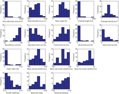
From the above-mentioned literature, the initial 14 sub-catchment properties used for this study were (1) sub-catchment area (A), (2) mean elevation of the sub-catchment (ELE), (3) mean slope of the sub-catchment (SLP), (4) channel length (CHL), (5) drainage density (DD), (6) % mountainous soil (%MS), (7) % agriculture (%AGR), (8) % forest (%FOR), (9) % mixed land use (i.e. mine, landfill, garbage dump, marsh and swamp) (%MIX), (10) % urban (%URB), (11) % open water (river, natural water resource, farm pond, canal, and reservoir) (%WAT), (12) mean annual rainfall (referring to the areal rainfall estimated by the rainfall gradient and inverse distance weighting method as described in Visessri and McIntyre 2012) (MAR), (13) mean wet month rainfall (similar to the estimation of mean annual rainfall but using the monthly averaged between May and October) (MWR), and (14) mean dry month rainfall (similar to the estimation of mean annual rainfall but using the monthly averaged over January–April and November–December) (MDR). While the potential influence of land-use change will be explored later, the regression assumes that the land use in 2000 sufficiently represents the land use between 1995 and 2006. For each sub-catchment, RC, BFI and EL were calculated using the observed rainfall–flow data from 1995–2006 and regression equations relating these indices to the sub-catchment properties were identified.

The original values of the properties and indices were transformed by subtracting their mean values (over the 44 sub-catchments) and dividing by their standard deviations. This resulted in zero mean and unit standard deviation of each property and each index. This allows the regression coefficients to be interpreted as relative sensitivity measures. Histograms representing the distribution of each of the indices are shown in Fig. 4. The analyses described in Sections 3 and 4 were applied using these data without transformation; however, the value of transforming the data will be discussed in Section 5.

Figure 4. Histograms for 14 sub-catchment properties and the three flow indices (RC, BFI and EL).

Using all 44 sub-catchments, the properties were related to the three flow indices using regression. Forward stepwise regression was employed in order to avoid high covariance between the regression coefficients, with the stepwise regression entrance and exit p-value tolerances set to 0.05. This approach leads to the potential problem that predictors that directly affect the flow indices may be excluded due to their high dependency on other predictors. In a compromise between optimising statistical significance and aiming to include the physically important predictors, equations produced by the stepwise regression were refined by removing the sub-catchment properties that contributed little to the r² value and also lacked clear physical connections to the indices.

3.3 Uncertainty estimation and validation

There are various sources of uncertainty in the regression (Kjeldsen and Jones 2010): (1) there are errors in the three observed indices, for example originating from error in converting water level to discharge and error in interpolating rainfall over a sub-catchment area; (2) there are errors in the measured sub-catchment properties, for example due to land-use change and sparseness of soil sampling; (3) the linear regression equation cannot represent the true nonlinear and time-dependent relationship between the sub-catchment properties and the indices; (4) there are likely to be relevant properties not included in the regression, because their effect was unidentifiable, or measurements of the properties were not available; and (5) there are only limited sets of observations (44 sets of sub-catchment properties and indices) available so the regression coefficients are only an approximation of the true optimal values. One of the motivations of this research is to explore the utility of regionalisation where these uncertainties are higher than in most published regionalisation studies. It is proposed that the combined effect of the sources of error in the regression can usefully be quantified by analysing the regression residuals, as is common practice (Brath et al. 2001, Kjeldsen and Jones 2010). The variance of the regression coefficients and of the regression residuals can be used to represent uncertainties caused by all error types listed above, on the assumption that the errors in the indices for any ungauged site are drawn from the same distribution estimated by the gauged site residuals. This is not necessarily a trivial assumption, as some sub-catchments may have distinctive types and sizes of errors, for example due to specific land-use changes or gauging errors.

For validating the success of the regression for estimating response indices, each of the 44 sub-catchments was removed one at a time as a test sub-catchment and the regression coefficients were estimated using the data from the remaining 43 sub-catchments. The explanatory properties were assumed to be the same (i.e. those identified using all 44 sub-catchments). Scatter plots are used to review the relationship between observed and predicted values of the indices.

3.4 Evaluation of land use change impacts

Between 1995 and 2006, several sub-catchments were partially converted from forest to agriculture, with a maximum conversion of 23%. At least three interesting questions arise: (1) How has the land-use change affected the flow indices?; (2) Is this observed change consistent with that predicted by the spatially-derived regression equations, in which case there is evidence that the spatial regressions can be used to predict non-stationarity effects (supporting the trading-space-for-time hypothesis of Peel and Blöschl (2011), Singh et al. (2011), Wagener and Montanari (2011), Bulygina et al. (2012))?; (3) To what extent has the land-use change increased uncertainty in the regionalisation? In order to answer the first of these questions, changes in observed indices were analysed between the periods (water years) 1995–2000 and 2001–2006. Relationships between the changes in indices and the changes in land-use properties were visually investigated. To answer the second question, any observed changes were compared with the corresponding changes that would be estimated using the spatially derived regression equations described in Sections 3.2 and 3.3. To answer the third question, the regionalisation analysis was repeated independently for the two 5-year time periods and then the differences in test sub-catchment predictions of indices were analysed.

3.5 The influence of data quality on regression performance

The final step is to investigate whether the performance in the test sub-catchment is linked to the quality of data in that sub-catchment. The influence of data quality in hydrological studies is something that is generally ignored or mentioned in passing without significant analysis. This is understandable given that data quality information is often absent or minimal, difficult to obtain from data providers, and/or it cannot easily be turned into quality metrics for the purpose of analysis. Here, a pragmatic, partly subjective scoring system is used to quantify data quality. Although partly subjective, it is the first attempt, in our knowledge, to quantify rainfall–flow data quality in Thailand and, more generally, to link data quality indicators to regionalisation performance.

The data quality score is the sum of the scores determined by the seven quality criteria shown in Table 2. Sub-catchment sizes and elevations are included in the criteria as they are believed to affect the ability to sample rainfall effectively. The range of scores for each criterion is based on the range and distribution of the values from all the test sub-catchments, and the perceived ability to distinguish between sub-catchments within these ranges. The possible aggregate score based on the criteria in Table 2 ranges from 7 to 46. The higher the score, the better the perceived data quality.

Table 2. Criteria for evaluating data quality of the test sub-catchments.

Criterion	Range of values	Range of scores	Comments
Length of flow record (years)	5–11	1–7	Excluding 1-year warm-up period. The flow record should be long enough to cover variation in seasonality. It should contain average, wet and dry years and not bias to particular years. The longer record thus implies smaller uncertainty in estimating regionalised flow indices.
Number of years of flow record overlapping with rainfall record (years)	5–11	1–7	Excluding 1-year warm up period.
Number of possible outliers in flow record (number/year)	0–4	1–5	Box plot analysis (excluding zero values) is used to identify outliers together with additional sources of information, which are historical flood reports produced by RID, Department of Disaster Prevention and Mitigation (DPM), and Hydro and Agro Informatics Institute (HAII).
Frequency of revision of rating curve	Rarely, Hardly, Regularly	1–3	This is based mainly on the information provided by local staff that the rating curves of main rivers should be regularly reviewed, corresponding to once per year. The rating curves of small rivers or tributaries are reviewed at lower frequency.
Missing rainfall data from rain gauge(s) located within the sub-catchment (%)	0–30	1–6	Total number of days of missing data from all rain gauge(s) located within the sub-catchment divided by the total number of days of rainfall record, multiplied by 100.
Sub-catchment sizes (km^2)	5–14 814	1–8	The wide range of the sub-catchment sizes is determined only by a few very large sub-catchments. To deal with the difference in order of magnitude, the sub-catchments are classified from the size less than the smallest order of magnitude (<10^1) to the size greater than or equal to the highest order of magnitude (≥10^4), with a half order of magnitude increase between the lower and upper classes, e.g. <10^1, 10^1–10^1.5, 10^1.5–10^2, …, ≥10^4. There are eight classes for the sub-catchment sizes and scores of 1 to 8 are given to each class in ascending order from the smallest to the largest.
Sub-catchment elevations (m a.s.l.)	624–1529	1–10	Elevations of the sub-catchments are divided into intervals of 100 m a.s.l. from <700 m a.s.l. to >1500 m a.s.l., resulting in 10 classes in total. Scores of 1 to 10 are given in ascending order from the lowest to the highest classes.

4 Results

4.1 Regression

When applying the stepwise regression to the 44 test sub-catchments, elevation was found to be statistically linked to all three indices. Elevation does not have a clear direct physical connection to the indices, and its inclusion may obscure the more direct effects, for example of slope, soil type, percentage mixed land use and percentage open water, due to their dependency on elevation (from Table 1, correlations of these four properties with elevation are 0.51, 0.62, −0.32 and −0.47, respectively). When the stepwise regression was repeated without including the elevation input, for BFI, %URB became significant and the r² remained unchanged to two decimal places at 0.42. However, without allowing elevation to be an input, the r² for RC was reduced from 0.81 to 0.54; and elevation was the only catchment property that significantly explained EL. Elevation is therefore considered necessary for predicting RC and EL, with the recognition that more direct physical effects cannot be distinguished. The coefficients and r² values are listed in Table 3.

Table 3. Identified regression equations.

Index	Regression inputs	1995–2006		2001–2006
		Standardised coefficient	Cumulative r^2	Standardised coefficient	Cumulative r^2
RC	Elevation (ELE)	0.82	0.45	0.81	0.41
	Mean annual rainfall (MAR)	−0.58	0.59	−0.59	0.47
	Mean dry month rainfall (MDR)	0.28	0.70	0.49	0.69
	%Urban land use (%URB)	0.32	0.76	0.23	0.69
	%Forest land use (%FOR)	0.23	0.81	0.27	0.73
BFI	Mean slope (SLP)	0.57	0.29	0.43	0.27
	%Urban land use (%URB)	−0.35	0.42	−0.28	0.34
EL	Elevation (ELE)	−0.39	0.15	−0.36	0.13

The physical interpretation of the statistically significant properties is not always straightforward, particularly for RC. For example, in Table 3, the coefficient for MAR is negative implying that, after taking out the effect of the other four explanatory variables, drier sub-catchments tend to have larger RC values. This result may be speculatively related to systematic data issues, such as the difficulty of estimating high flow rates and thus the underestimation of runoff coefficients in wetter areas. Another surprising result in Table 3 is that, after removing the influence of the other four explanatory variables, forested areas tend to have higher runoff coefficients. This may be because: (1) there are fewer abstractions and less irrigation in forested areas, overcoming the increased evaporation normally associated with forests (Calder and Aylward 2006); (2) forested area are usually converted to paddy fields which significantly increases surface storage (Praneetvatakul et al. 2001, Kim et al. 2005); and (3) underestimation of rainfall in forested areas, which are usually located at high elevations (Oudin et al. 2008a). Regarding BFI, the negative correlation between BFI and urban cover is expected. Table 3 also shows that sub-catchments with steep slopes tend to have higher BFI values. It is thought that slope implicitly represents the importance of mountainous soil (the correlation coefficient for these two properties is 0.78). While the properties of the mountainous soil type vary widely across the sub-catchments, it is believed that mountainous soils are able to absorb water well, thus inducing high BFI.

The coarse classification of different soil textures into one “mountainous soil” type prevents the regression from relating significant soil properties to BFI. If the “mountainous soil” type can be sub-categorised according to soil textures and soil depth, this may support identification of a more powerful regional model for BFI. However, for heterogeneous catchments, using information from soil databases may not be enough and additional properties may be needed for estimating BFI (Oudin et al. 2010). Similarly, the regression equation for EL provides little insight into the governing properties. The decrease in EL associated with increase in elevation is thought to be because flow at high elevations tends to have higher base flow due to the soil effects and thus is less seasonally variable.

The histograms in Fig. 5 and scatter plots in Fig. 6 show that the distributions of the regression residuals approximately follow normal distributions with no obvious heterogeneity of errors over the range of data. This satisfies the main assumptions implicit to the linear regression method, and allows uncertainty bounds to be reasonably approximated by the percentiles of a normal distribution. The uncertainty derived from the regression, aiming to include all error types described in Section 3.3, is represented by confidence and prediction intervals as shown in Fig. 6. The confidence intervals represent only the regression coefficient uncertainty, while the prediction intervals also include the error variance. From this figure it can be seen that almost all observed indices lie within their 95% prediction intervals, except for one sub-catchment for each index.

Figure 5. Histograms for the regression residuals of the three indices (RC, BFI and EL). The ranges of the data on the x-axis are equally divided into six bins.

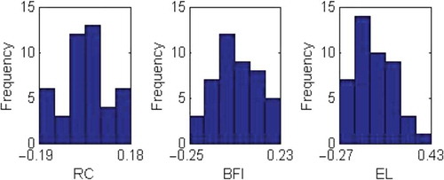
Figure 6. Regression fits and uncertainty intervals for 1995–2006. Uncertainty intervals for RC and BFI are not smooth because they are explained by more than one sub-catchment property.

4.2 Land-use change effects

Evaluation of land-use change impacts using the regression model is possible for RC and BFI but not EL, because the regression for predicting EL does not explicitly include any land-use property. This again highlights the limitation of the regionalisation approach, where land-use effects may be present but are not identifiable from the gauged sub-catchments given the various uncertainties and co-linearities.

Figure 7 aims to show how the observed RC, BFI and EL values have changed due to changes in forest cover. Figure 7(a) shows that the observed changes in forest cover have a weak negative correlation with the observed changes in RC between periods 1 and 2. This direction of change contradicts the regression shown in Table 3, potentially because the decrease of forest cover over time is generally coincident with an increase in urban cover. The change in RC for sub-catchments with unchanged forest cover, e.g. catchment 8 (in the, see northeast Fig. 1), as highlighted by a small circle in Fig. 7 and Fig. 8, may be due to the change in urban cover together with climate variability between the two periods. However, Fig. 8(a) provides little evidence that RC is systematically affected by changes in MAR. The land-use change impact on the observed BFI is shown in Fig. 7(b). The relationship appears weak, although significantly more of the test sub-catchments lie in the lower left quarter of the figure than in the upper left, showing that a decrease in forest cover tended to cause a decrease in BFI. Figure 8(b) shows that the increase in MAR over the two periods also tended to decrease BFI, although the effect appears marginal.

Figure 7. Impacts of forest cover change on the observed indices: (a) observed RC, (b) observed BFI, and (c) observed EL.

Figure 8. Impacts of mean annual rainfall change on the observed indices: (a) observed RC, (b) observed BFI, and (c) observed EL.

Figure 9 compares the observed changes in index values between the two periods with those predicted by the spatial regionalisation equations. Figure 9(a) suggests that the spatially-derived regression equation could be used to model the trend in RC over time, but with high uncertainty and also considerable bias. Figure 9(b) shows that the regression cannot predict the observed change in BFI: considering only the change in urban cover, as appeared in the regression, is not enough to represent the observed change in BFI. No change in EL was observed.

Figure 9. Relationship between the observed and predicted change in indices from period 1 to period 2: (a) RC, and (b) BFI. No change in EL was predicted.

Overall, it appears from this linear regression analysis that the spatial land-use signals in flow response are too weak and indistinguishable from other spatial effects to be helpful in predicting effects of change, with the possible exception of the effects on runoff volumes of the change of forest cover into urban area.

As a simple illustration of how much uncertainty the land-use change introduces to the regionalisation, the regression coefficients were re-estimated using the data from the post-change period of 2001–2006. Table 3 shows that the coefficients for 1995–2006 and for 2001–2006 are similar except for the MDR coefficient.

4.3 Effects of data quality

Using the criteria shown in Table 2 leads to a data quality score for the test sub-catchments that can be linked to the regression performance, as shown in Fig. 10. Figure 10(a) shows relatively small regression residuals (shown as absolute values) for predicting RC (as can be expected from the high r² shown in Table 3), but no connection between the data quality score and regression residuals can be found. There is stronger evidence that data quality affects the predictions of BFI and EL.

Figure 10. Relationship between data quality score and absolute value of regression residuals: (a) RC, (b) BFI, and (c) EL.

By excluding the seven test sub-catchments with the lowest data quality score, the uncertainty in the regression reduced slightly. For example, the maximum absolute values of the regression residuals for RC and BFI reduced to 0.18 and 0.23, respectively, compared to 0.19 and 0.25 when including all sub-catchments; and the standard deviations of the residuals for RC, BFI and EL improved from 0.058, 0.064 and 0.089 to 0.056, 0.060 and 0.086, respectively.

5 Discussion

This paper described a Thai case study of hydrological regionalisation by regressing flow response indices against available catchment property data. Although this is a well-established research area—see reviews in McMahon et al. (2013), Weingartner et al. (2013—this paper reports the most detailed regionalisation study yet conducted for Thailand that we are aware of (see also Schreider and Jakeman 1999, Schreider et al. 1999, 2002, Croke et al. 2004, Merritt et al. 2004, Dutta et al. 2006, Post and Hartcher 2006, Rojanamon et al. 2007, Mapiam and Sriwongsitanon 2009, Taesombat and Sriwongsitanon 2010, Piman and Babel 2013). The focus on using limited catchment property data and looking quantitatively at effects of data quality on regionalisation performance are also new contributions of the paper. Furthermore, the paper tests whether the spatial regionalisation can be applied to predicting the effects of deforestation on river flows.

The three flow indices regionalised were the runoff coefficient (RC), the base flow index (BFI) and the flow seasonal elasticity (EL). The RC was well explained by the regression, with an r² value of 0.81, a result which itself is useful for water resources planning in ungauged areas where only the long-term average flow estimates are needed. The predictability of BFI from the catchment properties was poor, with a regression r² of 0.42. This r² value is poor compared to other published results (Haberlandt et al. 2001, Mehaiguene et al. 2012); nevertheless, is sufficient to provide some useful information about expected hydrograph shapes and low flows in ungauged areas. The estimation of uncertainty in RC and BFI using the confidence and prediction intervals provides information about the reliability with which they can be applied. The predictability of EL was rather poor, with an r² of only 0.15, meaning that the inter-seasonal variability of the flow response is difficult to predict using linear regression, which places constraints on the applicability to water resources applications. The uncertainty in estimation of the indices from the catchment property data stems from a combination of things, listed earlier in the paper. The predominant sources of uncertainty seem likely to be the limitations in the accuracy of the rainfall and flow gauging; the absence of abstraction data; and limitations in the available soils and geology properties. The soil property data, which generally feature in regionalisation equations (McMahon et al. 2013, Weingartner et al. 2013), were restricted to the percentages of soil considered to be “mountainous” in each catchment, and the influence of this soil type was not identified in any of the regression equations.

The spatial signals of land-use effects were weak (Table 3). Climate effects dominated over land-use effects for RC, and slope effects dominated for BFI, and there were no signals of land use in the EL equation (although they may be implicit to the effects of elevation, which is correlated with land use in the case study). The significant amount of deforestation that occurred in the study period, 1995–2006, was accompanied by significant changes in the RC, BFI and EL values. However, no clear relationships between degree of deforestation and the three indices were found, and the regionalisation equations could not be used to help predict the effects of deforestation except, to a small degree, for RC. The changes in indices were more linked to changes in rainfall, especially wet month rainfall, over the two periods. This is because rainfall in monsoon-dominated areas is strongly variable and more distinguishable than changes in land-use. It seems that there are temporal influences on the observed index values in individual catchments that are not captured in the regionalisation exercise, such as local changes to land-use management, abstractions and gauging bias. The ambiguity in the physical significance of the regression equations in Table 3, due to co-linearity of predictors, also affects their ability to predict effects of change. This result indicates the dangers of translating simple spatial analysis based on limited data sets to predict the complex effects of future change. Studies using longer-term data sets and larger spatial databases with a greater number of independent catchments that better elucidate the physical influences of land use may help overcome this problem (Oudin et al. 2008b). Given the lack of evidence in the catchment-scale observations, expert knowledge based on international studies and physics-based modelling may need to be introduced to predict land-use effects (Merz and Blöschl 2008, Buytaert and Beven 2009, Bulygina et al. 2012, Fraser et al. 2013).

A partly subjective data quality score was devised (Table 2) and was found to be useful in explaining regression model performance. Poor data quality deteriorates regionalisation performance, especially for small catchments at high elevations where the estimation of rainfall is difficult and where rainfall has a stronger influence on flow. Figure 10 indicates that the magnitude of regression residuals for BFI and EL reduce by around 0.1 when moving from the test catchments with the worst quality data to those with the best. Therefore this type of data quality analysis is potentially useful in setting priorities for data collection and quality control in Thailand and beyond, and could be used to implement a refined, weighted regression approach. The unclear relationship between data quality score and the regression residuals for RC (Fig. 10(a)) is believed to be caused by the criteria used for defining the data quality score. Further work is therefore needed to test sensitivity to the data quality scoring system. Also, formalising some of the key uncertainties, for example through stochastic rainfall modelling and rating curve statistical analysis, would reduce the qualitative aspects.

The results presented above do not address the possible improvements in precision or interpretability of the regression that may be achieved using transformations of the data. The validity of the regression is partly justified by the approximately normal distributions of errors shown in Fig. 5; however, the histograms in Fig. 4 show that some of the predictors have positively skewed distributions implying that applying a Box-Cox transform to the predictors may achieve better stepwise regression results. When the stepwise regression was repeated using Box-Cox transformed predictors, the values of r² for RC and BFI were similar to those in Table 3, and the r² for EL was improved to 0.49 from 0.15. Mixed land use (%MIX) became an important predictor for RC, with forest and urban cover being eliminated, introducing the possibility that the presence of swamps and wetlands may reduce RC. Open water (%WAT) became an important predictor for EL with elevation being eliminated, suggesting that surface storage in this case study enhances the differences in rainfall–runoff response between wet and dry seasons (potentially due to retention of low flows). When using the spatial regionalisation equations developed from Box-Cox transformed data to evaluate the land-use change impact, no relationships between the observed and predicted changes in index values between the two periods were found. Thus the introduction of the Box-Cox transform illustrates that the terms in the regression equations may be sensitive to assumptions about linearity, and this clearly has implications for interpretation and prediction.

In terms of other general priorities for improving the accuracy of modelling the hydrology of ungauged areas of Thailand, more research on rainfall estimation especially for mountainous catchments, is needed to characterise and reduce rainfall estimation error. For example, satellite and radar data could be used together with point rain gauges to improve the temporal and spatial accuracies (Collier 1986a, 1986b, Xie and Arkin 1996, Grimes et al. 1999, Todini 2004, Hughes 2006a, Ward et al. 2011). Rainfall downscaling could potentially be applied to convert satellite data into catchment-scale estimates with uncertainty. Regarding flow estimation, a review of flow gauges and identification of which gauges should be invested in are needed. Also, observed flow data should ideally be naturalised by taking into account abstraction and effluent estimates. If collecting the data needed for flow naturalisation is impractical, some estimates of seasonally averaged abstractions associated with different land uses would be helpful to reduce uncertainty in the regionalisation, especially about effects of deforestation. The uncertainty over abstractions is thought to be a primary reason for the uncertainty in the regression of RC and the influence of deforestation on RC, and thus affects ability to plan regional water resources and land use management. Another priority for improved hydrological modelling of ungauged areas in Thailand is the development of soils databases that include hydrologically relevant property data (e.g. Boorman et al. 1995).

6 Conclusions

This paper reports a regionalisation analysis that aims to support water resources planning in northern Thailand. Results of a stepwise linear regression analysis on 44 gauged sub-catchments showed that the observed spatial variability of two important hydrological indices—the runoff coefficient and base flow index—could be explained by catchment properties with reasonable (given data quality) precision; however, the physical factors governing the indices were not necessarily represented well by the regression. In particular, we were not confident that the land-use influences on hydrological responses were represented. Where significant deforestation occurred during the study period, the regression equations failed to predict well the observed changes in flow response. There was a visually identifiable relationship between a catchment’s data quality metric and the performance of the regionalisation model in that catchment; however, the effect of land use non-stationarity on performance was unclear. It is concluded that significant investment in improved hydrological gauging, soils data and abstraction estimation may be needed to further refine regionalisation models and to isolate signals of land-use change from those of climatic variability. Further insight would be gained by extending the study to include basins in the same hydro-climatic region.

Acknowledgements

The authors would like to thank to the Thai Meteorological Department, the Royal Irrigation Department, the Department of Water Resources, and the Land Development Department for providing data for this study. The Hydrology and Water Management Centre for Upper Northern Region is acknowledged for useful discussion. We thank the reviewers for their constructive comments that helped improve the paper.

Disclosure statement

No potential conflict of interest was reported by the authors.

Additional information

Funding

The financial support from the Ministry of Science and Technology, Thailand for the first author is also acknowledged.

References

- Almeida, S., et al., 2012. Predicting flows in ungauged catchments using correlated information sources. In: BHS 11th National symposium: hydrology for a changing world, 9–11 July 2012 Dundee, UK.
- Bao, Z., et al., 2012. Comparison of regionalization approaches based on regression and similarity for predictions in ungauged catchments under multiple hydro-climatic conditions. Journal of Hydrology, 466–467 (0), 37–46. doi:10.1016/j.jhydrol.2012.07.048
- Bari, M.A., et al., 1996. Changes in streamflow components following logging and regeneration in the southern forest of Western Australia. Hydrological Processes, 10 (3), 447–461. doi:10.1002/(SICI)1099-1085(199603)10:3<447::AID-HYP431>3.0.CO;2-1
- Boorman, D.B., Hollist, J.M., and Lilly, A., 1995. Hydrology of soil types: a hydrologically-based classification of the soils of the United Kingdom. Wallingford, UK: Institute of Hydrology.
- Boughton, W. and Chiew, F.H.S., 2007. Estimating runoff in ungauged catchments from rainfall, PET and the AWBM model. Environmental Modelling & Software, 22 (4), 476–487. doi:10.1016/j.envsoft.2006.01.009
- Brath, A., et al., 2001. Estimating the index flood using indirect methods. Hydrological Sciences Journal, 46 (3), 399–418. doi:10.1080/02626660109492835
- Brown, J.D. and Heuvelink, G.B.M., 2006. Assessing uncertainty propagation through physically based models of soil water flow and solute transport. Encyclopedia of Hydrological Sciences, 6, 79. John Wiley & Sons, Ltd. doi:10.1002/0470848944.hsa081.
- Bulygina, N., et al., 2012. Integrating different types of information into hydrological model parameter estimation: application to ungauged catchments and land use scenario analysis. Water Resources Research, 48 (6), W06519. doi:10.1029/2011WR011207
- Bulygina, N., McIntyre, M., and Wheater, H., 2009. Conditioning rainfall-runoff model parameters for ungauged catchments and land management impacts analysis. Hydrology and Earth System Sciences, 13, 893–904. doi:10.5194/hess-13-893-2009
- Bulygina, N., McIntyre, N., and Wheater, H., 2011. Bayesian conditioning of a rainfall–runoff model for predicting flows in ungauged catchments and under land use changes. Water Resources Research, 47 (2), W02503. doi:10.1029/2010WR009240
- Burn, D.H. and Boorman, D.B., 1993. Estimation of hydrological parameters at ungauged catchments. Journal of Hydrology, 143 (3–4), 429–454. doi:10.1016/0022-1694(93)90203-L
- Buytaert, W. and Beven, K.J., 2009. Regionalization as a learning process. Water Resources Research, 45 (11), W11419. doi:10.1029/2008WR007359
- Calder, I.R. and Aylward, B., 2006. Forest and floods: moving to an evidence-based approach to watershed and integrated flood management. Water International, 31 (1), 87–99. doi:10.1080/02508060608691918
- Chiew, F.H.S., 2006. Estimation of rainfall elasticity of streamflow in Australia. Hydrological Sciences Journal, 51 (4), 613–625. doi:10.1623/hysj.51.4.613
- Chiew, F.H.S., et al., 2009. Estimating climate change impact on runoff across southeast Australia: method, results, and implications of the modeling method. Water Resources Research, 45 (10), W10414. doi:10.1029/2008WR007338
- Collier, C.G., 1986a. Accuracy of rainfall estimates by radar, part I: calibration by telemetering raingauges. Journal of Hydrology, 83 (3–4), 207–223. doi:10.1016/0022-1694(86)90152-6
- Collier, C.G., 1986b. Accuracy of rainfall estimates by radar, part II: comparison with raingauge network. Journal of Hydrology, 83 (3–4), 225–235. doi:10.1016/0022-1694(86)90153-8
- Croke, B.F.W., Merritt, W.S., and Jakeman, A.J., 2004. A dynamic model for predicting hydrologic response to land cover changes in gauged and ungauged catchments. Journal of Hydrology, 291 (1–2), 115–131. doi:10.1016/j.jhydrol.2003.12.012
- Croke, B.F.W. and Norton, J.P., 2004. Regionalisation of rainfall-runoff models. In: C. Pahl, et al., ed. 2nd biennial meeting of the international environmental modelling and software society., 14–17 June 2004. University of Osnabruck, Germany. Manno, Switzerland: International Environmental Modelling and Software Society, 1201–1207.
- Cutore, P., et al., 2007. Regional models for the estimation of streamflow series in ungauged basins. Water Resources Management, 21, 789–800. doi:10.1007/s11269-006-9110-7
- Department of Mineral Resources, 2010. Geology of Thailand [online]. Bangkok, Thailand: Ministry of Natural Resources and Environment. Available from: http://www.dmr.go.th/ewtadmin/ewt/dmr_web/main.php?filename=GeoThai_En [Accessed 29 December 2010].
- Dutta, D., Chaleeraktrakoon, C., and Budhakooncharoen, S., 2006. Research initiatives in Thailand on predictions in ungauged basins. In: M. Sivapalan, et al., eds Prediction in ungauged basins: promise and progress. Wallingford, UK: IAHS Press, 492–504.
- Fernandez, W., Vogel, R.M., and Sankarasubramanian, A., 2000. Regional calibration of a watershed model. Hydrological Sciences Journal, 45 (5), 689–707. doi:10.1080/02626660009492371
- Fraser, C.E., et al., 2013. Upscaling hydrological processes and land management change impacts using a metamodeling procedure. Water Resources Research, 49 (9), 5817–5833. doi:10.1002/wrcr.20432
- Gibbs, M.S., Maier, H.R., and Dandy, G.C., 2012. A generic framework for regression regionalization in ungauged catchments. Environmental Modelling & Software, 27–28 (0), 1–14. doi:10.1016/j.envsoft.2011.10.006
- Grimes, D.I.F., Pardo-Igúzquiza, E., and Bonifacio, R., 1999. Optimal areal rainfall estimation using raingauges and satellite data. Journal of Hydrology, 222 (1–4), 93–108. doi:10.1016/S0022-1694(99)00092-X
- Haberlandt, U., et al., 2001. Regionalisation of the base flow index from dynamically simulated flow components—a case study in the Elbe River Basin. Journal of Hydrology, 248 (1–4), 35–53. doi:10.1016/S0022-1694(01)00391-2
- He, Y., Bardossy, A., and Zehe, E., 2011. A review of regionalisation for continuous streamflow simulation. Hydrology and Earth System Sciences, 15, 3539–3553. doi:10.5194/hess-15-3539-2011
- Heuvelmans, G., Muys, B., and Feyen, J., 2006. Regionalisation of the parameters of a hydrological model: comparison of linear regression models with artificial neural nets. Journal of Hydrology, 319 (1–4), 245–265. doi:10.1016/j.jhydrol.2005.07.030
- Hrachowitz, M., et al., 2013. A decade of predictions in ungauged basins (PUB)—a review. Hydrological Sciences Journal, 58 (6), 1–58. doi:10.1080/02626667.2013.803183
- Hughes, D.A., 2006. Comparison of satellite rainfall data with observations from gauging station networks. Journal of Hydrology, 327 (3–4), 399–410. doi:10.1016/j.jhydrol.2005.11.041
- Hughes, D.A., et al., 2006. Regional calibration of the Pitman model for the Okavango River. Journal of Hydrology, 331 (1–2), 30–42. doi:10.1016/j.jhydrol.2006.04.047
- Hughes, D.A., Kapangaziwiri, E., and Sawunyama, T., 2010. Hydrological model uncertainty assessment in southern Africa. Journal of Hydrology, 387 (3–4), 221–232. doi:10.1016/j.jhydrol.2010.04.010
- Kapangaziwiri, E. and Hughes, D., 2008. Towards revised physically based parameter estimation methods for the Pitman monthly rainfall-runoff model. Water SA, 34 (2), 183–192.
- Kapangaziwiri, E., Hughes, D., and Wagener, T., 2009. Towards the development of a consistent uncertainty framework for hydrological predictions in South Africa. In: K. Yilmaz, ed. New approaches to hydrological predictions in data-sparse regions. Wallingford, UK: International Association of Hydrological Sciences, IAHS Publ. 333, 84–93. Available online at: http://iahs.info/uploads/dms/iahs_333_0084.pdf
- Kapangaziwiri, E., Hughes, D.A., and Wagener, T., 2012. Incorporating uncertainty in hydrological predictions for gauged and ungauged basins in southern Africa. Hydrological Sciences Journal, 57 (5), 1000–1019. doi:10.1080/02626667.2012.690881
- Kim, U. and Kaluarachchi, J.J., 2008. Application of parameter estimation and regionalization methodologies to ungauged basins of the Upper Blue Nile River Basin, Ethiopia. Journal of Hydrology, 362 (1–2), 39–56. doi:10.1016/j.jhydrol.2008.08.016
- Kim, W., et al., 2005. Simulation of potential impacts of land use/cover changes on surface water fluxes in the Chaophraya river basin, Thailand. Journal of Geophysical Research: Atmospheres, 110 (D8), D08110. doi:10.1029/2004JD004825
- Kjeldsen, T.R. and Jones, D.A., 2010. Predicting the index flood in ungauged UK catchments: on the link between data-transfer and spatial model error structure. Journal of Hydrology, 387 (1–2), 1–9. doi:10.1016/j.jhydrol.2010.03.024
- Kokkonen, T.S., et al., 2003. Predicting daily flows in ungauged catchments: model regionalization from catchment descriptors at the Coweeta Hydrologic Laboratory, North Carolina. Hydrological Processes, 17 (11), 2219. doi:10.1002/hyp.1329
- Kumar, R., Livneh, B., and Samaniego, L., 2013. Toward computationally efficient large-scale hydrologic predictions with a multiscale regionalization scheme. Water Resources Research, 49 (9), 5700–5714. doi:10.1002/wrcr.20431
- Land Development Department, 2006. Land use map. Bangkok, Thailand: Ministry of Agriculture and Cooperatives.
- Li, H., et al., 2009. Predicting runoff in ungauged catchments by using Xinanjiang model with MODIS leaf area index. Journal of Hydrology, 370 (1–4), 155–162. doi:10.1016/j.jhydrol.2009.03.003
- Mapiam, P.P. and Sriwongsitanon, N., 2009. Estimation of the URBS model parameters for flood estimation of ungauged catchments in the upper Ping River basin, Thailand. ScienceAsia, 35, 49–56. doi:10.2306/scienceasia1513-1874.2009.35.049
- Maréchal, D. and Holman, I.P., 2005. Development and application of a soil classification-based conceptual catchment-scale hydrological model. Journal of Hydrology, 312 (1–4), 277–293. doi:10.1016/j.jhydrol.2005.02.018
- Mazvimavi, D., et al., 2005. Prediction of flow characteristics using multiple regression and neural networks: A case study in Zimbabwe. Physics and Chemistry of the Earth, Parts A/B/C, 30 (11–16), 639–647. doi:10.1016/j.pce.2005.08.003
- Mazvimavi, D., Meijerink, A.M.J., and Stein, A., 2004. Prediction of base flows from basin characteristics: a case study from Zimbabwe. Hydrological Sciences Journal, 49 (4), 703–715. doi:10.1623/hysj.49.4.703.54428
- McIntyre, N. and Marshall, M., 2010. Identification of rural land management signals in runoff response. Hydrological Processes, 24 (24), 3521–3534. doi:10.1002/hyp.7774
- McIntyre, N., et al., 2014. Modelling the hydrological impacts of rural land use change. Hydrology Research, 45 (6), 737–754. doi:10.2166/nh.2013.145
- McIntyre, N., et al., 2005. Ensemble predictions of runoff in ungauged catchments. Water Resources Research, 41 (12), W12434. doi:10.1029/2005WR004289
- McMahon, T.A., et al., 2013. Prediction of annual runoff in ungauged basins. In: G. Blöschl, et al., eds. Runoff prediction in ungauged basins. Cambridge: Cambridge University Press, 70–101.
- Mehaiguene, M., et al., 2012. Low flows quantification and regionalization in North West Algeria. Journal of Arid Environments, 87 (0), 67–76. doi:10.1016/j.jaridenv.2012.07.014
- Merritt, W.S., et al., 2004. A biophysical toolbox for assessment and management of land and water resources in rural catchments in Northern Thailand. Ecological Modelling, 171 (3), 279–300. doi:10.1016/j.ecolmodel.2003.08.010
- Merz, R. and Blöschl, G., 2004. Regionalisation of catchment model parameters. Journal of Hydrology, 287 (1–4), 95–123. doi:10.1016/j.jhydrol.2003.09.028
- Merz, R. and Blöschl, G., 2008. Flood frequency hydrology: 1. Temporal, spatial, and causal expansion of information. Water Resources Research, 44 (8), W08432. doi:10.1029/2007WR006744
- Merz, R. and Blöschl, G., 2009. A regional analysis of event runoff coefficients with respect to climate and catchment characteristics in Austria. Water Resources Research, 45 (1), W01405. doi:10.1029/2008WR007163
- Nathan, R.J. and McMahon, T.A., 1992. Estimating low flow characteristics in ungauged catchments. Water Resources Management, 6 (2), 85–100. doi:10.1007/BF00872205
- Oudin, L., et al., 2008a. Has land cover a significant impact on mean annual streamflow? An international assessment using 1508 catchments. Journal of Hydrology, 357 (3–4), 303–316. doi:10.1016/j.jhydrol.2008.05.021
- Oudin, L., et al., 2008b. Spatial proximity, physical similarity, regression and ungaged catchments: A comparison of regionalization approaches based on 913 French catchments. Water Resources Research, 44 (3), W03413. doi:10.1029/2007WR006240
- Oudin, L., et al., 2010. Are seemingly physically similar catchments truly hydrologically similar? Water Resources Research, 46 (11), W11558. doi:10.1029/2009WR008887
- Pallard, B., Castellarin, A., and Montanari, A., 2009. A look at the links between drainage density and flood statistics. Hydrology and Earth System Sciences, 13, 1019–1029. doi:10.5194/hess-13-1019-2009
- Peel, M.C. and Blöschl, G., 2011. Hydrological modelling in a changing world. Progress in Physical Geography, 35 (2), 249–261. doi:10.1177/0309133311402550
- Piman, T. and Babel, M.S., 2013. Prediction of rainfall-runoff in an ungauged basin: case study in the mountainous region of Northern Thailand. Journal of Hydrologic Engineering, 18 (2), 285–296. doi:10.1061/(ASCE)HE.1943-5584.0000573
- Post, D.A. and Hartcher, M.G., 2006. Evaluating uncertainty in modelled sediment delivery in data-sparse environments: application to the Mae Chaem catchment, Thailand. In: M. Sivapalan, ed. Prediction in ungauged basins: promises and progress. Wallingford, UK: International Association of Hydrological Sciences, IAHS Publ. 303, 80–89. Available online from: http://iahs.info/uploads/dms/13420.15-80-89-S7-W7-Post.pdf
- Praneetvatakul, S., et al., 2001. Assessing the sustainability of agriculture: a case of Mae Chaem Catchment, northern Thailand. Environment International, 27 (2–3), 103–109. doi:10.1016/S0160-4120(01)00068-X
- Reichl, J.P.C., et al., 2009. Optimization of a similarity measure for estimating ungauged streamflow. Water Resources Research, 45 (10), W10423. doi:10.1029/2008WR007248
- Rojanamon, P., Chaisomphob, T., and Rattanapitikon, W., 2007. Regional flow duration model for the Salawin River basin of Thailand. ScienceAsia, 33 (4), 411–419. doi:10.2306/scienceasia1513-1874.2007.33.411
- Royal Irrigation Department, 2003. The status of the 25 River basins. Bangkok, Thailand: Ministry of Agriculture and Cooperatives.
- Schreider, S.Y., et al., 1999. Hydrologic component of a DSS for sustainable development of Northern Thailand highland catchments. In: 2nd International conference on multiple objective decision support systems (MODSS99), Brisbane, Australia.
- Schreider, S.Y., et al., 2002. Prediction of monthly discharge in ungauged catchments under agricultural land use in the Upper Ping basin, Northern Thailand. Mathematics and Computers in Simulation, 59 (1–3), 19–33. doi:10.1016/S0378-4754(01)00390-1
- Schreider, S.Y. and Jakeman, A.J., 1999. Surface runoff modelling in ungauged subcatchment of the Mae Chaem catchment, Northern Thailand: part I, methodology. In: L. Oxley and F. Scrimgeour, ed. International Congress on Modelling and Simulation MODSIM99. 6–9 December 1999. University of Waikato. Hamilton, New Zealand: Modelling and Simulation Society of Australia and New Zealand, 81–86.
- Sefton, C.E.M. and Boorman, D.B., 1997. A regional investigation of climate change impacts on UK streamflows. Journal of Hydrology, 195 (1–4), 26–44. doi:10.1016/S0022-1694(96)03257-X
- Sefton, C.E.M. and Howarth, S.M., 1998. Relationships between dynamic response characteristics and physical descriptors of catchments in England and Wales. Journal of Hydrology, 211 (1–4), 1–16. doi:10.1016/S0022-1694(98)00163-2
- Sikorska, A.E., et al., 2012. Bayesian uncertainty assessment of flood predictions in ungauged urban basins for conceptual rainfall-runoff models. Hydrology and Earth System Sciences, 16 (4), 1221–1236. doi:10.5194/hess-16-1221-2012
- Singh, R., et al., 2011. A trading-space-for-time approach to probabilistic continuous streamflow predictions in a changing climate – accounting for changing watershed behavior. Hydrology and Earth System Sciences, 15, 3591–3603. doi:10.5194/hess-15-3591-2011
- Taesombat, W. and Sriwongsitanon, N., 2010. Flood investigation in the upper Ping River basin using mathematical models. Kasetsart Journal, 44, 152–166.
- Thanapakpawin, P., et al., 2007. Effects of landuse change on the hydrologic regime of the Mae Chaem River basin, NW Thailand. Journal of Hydrology, 334 (1–2), 215–230. doi:10.1016/j.jhydrol.2006.10.012
- Todini, E., 2004. Role and treatment of uncertainty in real-time flood forecasting. Hydrological Processes, 18 (14), 2743–2746.
- Visessri, S. and McIntyre, N., 2012. Comparison between the TRMM product and rainfall interpolation for prediction in ungauged catchments. In: R. Seppelt, et al., ed. 6th biennial meeting of the international environmental modelling and software society, 1–5 July 2012. Leipzig, Germany: International Environmental Modelling and Software Society. Available from: http://www.iemss.org/society/index.php/iemss-2012-proceedings:
- Wagener, T., 2007. Can we model the hydrological impacts of environmental change? Hydrological Processes, 21 (23), 3233–3236. doi:10.1002/hyp.6873
- Wagener, T. and Montanari, A., 2011. Convergence of approaches toward reducing uncertainty in predictions in ungauged basins. Water Resources Research, 47 (6), W06301. doi:10.1029/2010WR009469
- Wagener, T. and Wheater, H., 2006. Parameter estimation and regionalization for continuous rainfall-runoff models including uncertainty. Journal of Hydrology, 320 (1–2), 132–154. doi:10.1016/j.jhydrol.2005.07.015
- Wagener, T., Wheater, H., and Gupta, H.V., 2004. Rainfall-runoff modelling in gauged and ungauged catchments. London: Imperial College Press.
- Ward, E., et al., 2011. Evaluation of precipitation products over complex mountainous terrain: A water resources perspective. Advances in Water Resources, 34 (10), 1222–1231. doi:10.1016/j.advwatres.2011.05.007
- Weingartner, R., et al., 2013. Prediction of seasonal runoff in ungauged basins. In: G. Blöschl, et al., eds. Runoff prediction in ungauged basins. Cambridge: Cambridge University Press, 102–134.
- Winsemius, H.C., et al., 2009. On the calibration of hydrological models in ungauged basins: a framework for integrating hard and soft hydrological information. Water Resource Research, 45, W12422. doi:10.1029/2009WR007706
- WMSC (Water Watch and Monitoring System for Warning Center), 2010. Summary of water condition in reserviors in. Thailand. Bangkok, Thailand: Ministry of Agriculture and Cooperatives.
- Wongprayoon, T. and Saengsrichan, W., 2004. Geology of the upper Ping basin. Unpublished report. Department of Minerals Resources, Thailand.
- Xie, P. and Arkin, P.A., 1996. Analyses of global monthly precipitation using gauge observations, satellite estimates, and numerical model predictions. Journal of Climate, 9 (4), 840–858. doi:10.1175/1520-0442(1996)009<0840:AOGMPU>2.0.CO;2
- Yadav, M., Wagener, T., and Gupta, H.V., 2007. Regionalization of constraints on expected watershed response behavior for improved predictions in ungauged basins. Advances in Water Resources, 30 (8), 1756–1774.
- Young, A.R., 2006. Stream flow simulation within UK ungauged catchments using a daily rainfall-runoff model. Journal of Hydrology, 320 (1–2), 155–172. doi:10.1016/j.jhydrol.2005.07.017
- Zhang, Y. and Chiew, F.H.S., 2009. Evaluation of regionalisation methods for predicting runoff in ungauged catchments in Southeast Australia. In: 18th World IMACS/MODSIM congress, 13–17 July 2009 Cairns, Australia. 3442–3448.
- Zhang, Z., et al., 2008. Reducing uncertainty in predictions in ungauged basins by combining hydrologic indices regionalization and multiobjective optimization. Water Resources Research, 44 (12), W00B04. doi:10.1029/2008WR006833