Uncovering global climate fields causing local precipitation extremes

ABSTRACT

Earlier studies have focused on establishing the hydroclimatic teleconnection between hydrological extremes and a single or a few preselected coupled oceanic–atmospheric circulation patterns (OACP). In this study, we hypothesise that local (continental-scale) hydrological extremes are, in general, influenced by a concurrent effect of different climate variables from several regions across the globe. The suite of these variables is termed the global climate pattern (GCP) behind the target hydrological event. To explore our hypothesis, we considered monthly Indian rainfall, which is a complex, continental-scale hydrological phenomenon. Extreme events are identified through the standardized precipitation anomaly index (SPAI), used as an indicator of dry and wet events. The global fields of different climate variables—sea surface temperature (SST), surface pressure (SP), air temperature (AT), wind speed (WS) and total precipitable water (TPW)—are explored for possible revelatory patterns. In all, 15 different variables, each designated by a climate anomaly from a distinct zone on the globe, are found to form a potential global climate signal pool, which can be designated as the GCP for Indian rainfall. The combined information extracted from this GCP is proven to be highly efficient in predicting dry and wet events in Indian rainfall.

EDITOR Z. W. Kundzewicz; ASSOCIATE EDITOR G. Di Baldassarre

KEYWORDS:

• hydroclimatology
• hydroclimatic teleconnections
• global climate pattern (GCP)
• precipitation extremes
• Indian rainfall

1 Introduction

Past research has established the presence of a hydroclimatic teleconnection between large-scale atmospheric–oceanic circulation patterns and hydrological variables, particularly the impacts of El Niño-Southern Oscillation (ENSO) on the rainfall anomalies across the world (Nicholls 1983, Kousky et al. 1984). Most studies since then, including the very recent ones, have scrutinized the multidimensional role of specific oceanic–atmospheric phenomena, such as ENSO, Equatorial Indian Ocean Oscillation (EQUINOO), Pacific Decadal Oscillation (PDO), Atlantic Multidecadal Oscillation (AMO), Indian Ocean Dipole (IOD), North Atlantic Oscillation (NAO), etc. in influencing hydrological variables worldwide (Chiew and McMahon 2002, Terray et al. 2003, Gadgil et al. 2004, Goswami et al. 2006, Maity and Nagesh Kumar 2006, 2008, Feng and Hu 2008, Li et al. 2008, Mo and Schemm 2008, Ting et al. 2011, Singhrattna et al. 2012, Oubeidillah et al. 2012, Jiang et al. 2013, Rogers 2013, Wang et al. 2013). For instance, the influence of ENSO and AMO has been established in relation to the variability of China’s summer precipitation (Gu et al. 2009, Ye 2014) as well as the frequency of its extreme precipitation events (Fu et al. 2013). The direct role of ENSO in the biennial relationship of rainfall variability between Central and equatorial South America has been identified (Wu and Zhang 2010). The effect of NAO on hydroclimatic conditions in the Mediterranean region was discovered to be far-reaching—affecting winter precipitation, river flow and temperature (Brandimarte et al. 2011). Changes in large-scale circulation patterns were found to be responsible for the observed long-term warming and drying in central Europe (Philipp et al. 2007). Observed changes in the frequency and intensity of precipitation extremes in Europe are now largely explained by the persistence in atmospheric circulation patterns over the North Atlantic (Willems 2013). Recent studies have brought to focus the asymmetry in the response of rainfall anomalies in different parts of the world due to opposite phases of low variability oceanic circulation patterns (King et al. 2013, Qiu et al. 2014). Diverse studies have been conducted recently to explore various aspects of hydroclimatic teleconnections in the context of Indian hydroclimatology. Contrary to the previous findings of an inverse ENSO–ISMR (Indian summer monsoon rainfall) relationship, Panda et al. (2013) found a direct relationship for the rainfall and streamflow series with ENSO for the Mahanadi River basin in southern India. Francis and Gadgil (2013) introduced new indices for EQUINOO based on the anomaly of outgoing longwave radiation (OLR)/precipitation between eastern and western parts of the equatorial Indian Ocean. Krishnamurthy and Krishnamurthy (2013) studied the associations of decadal-scale oscillations in Indian rainfall with PDO, AMO and the Atlantic tripole oscillation.

Figure 1. Flowchart showing logical combinations of the outputs of two SVMs to obtain final predicted category of hydrological events. (CBD: cannot be determined.)

The role of climatic circulations in shaping regional hydrology is ever evolving (Abram et al. 2007, Cai and Vanrensch 2012), as is evident from the weakening of the ENSO–ISMR relationship over the years (Krishna Kumar 1999, Viswambharan and Mohanakumar 2014). Further, it is argued that the anomalies in circulation are themselves not the causes of hydrological extremes, rather they are the manifestations of a more complicated forcing mechanism (Shelton 2009). Considering that the memory carried by the atmosphere hardly exceeds a month, the underlying reason for the persistence of atmospheric features that are linked with extremes, particularly droughts, are still largely unknown (Hoerling 2003). In the absence of specific knowledge about the causal agents, the synoptic-scale climate features act as precursors/indicators and are vital sources of information for drought planning and management in the context of modern day water stress. Besides the large-scale circulation patterns, the complexity of hydroclimatic association is further increased at smaller spatio-temporal scales due to the influence of local meteorological variables (Maity and Kashid 2010, 2011). Increased air temperature and changes in relative humidity, evaporation and land-use pattern are known to trigger or enhance the drought events (Giannini et al. 2008, Wong et al. 2011, Maity et al. 2013). Persistent above-normal surface temperatures, which increased the moisture demand, are known to have aggravated the moisture deficits during the sweeping droughts over the Northern Hemisphere in 1998–2002 (Hoerling 2003). Thus, the contribution of local and global factors in moulding regional hydrological extremes is intricate and dynamic.

It is observed that most of the previous studies have dealt with the role of specific coupled oceanic–atmospheric circulation patterns (OACPs) that impacted rainfall anomalies causing droughts/floods. In these studies, the focus is on establishing triggers of precipitation extremes from a single or a few preselected coupled OACPs. However, we claim that such factors need not be limited by specific one or two identified OACPs. Rather, they can be more extensive and possibly innumerable. We hypothesise that a specific regional hydrological phenomenon is, in general, influenced by the concurrent effect of a specific global climate pattern (GCP). Such GCPs can be distinguished by the status of different climate variables from different regions across the globe. The objective of this study is to explore this hypothesis. We attempt to explore the entire global fields of six climatic variables to identify and evaluate the potential of GCPs influencing Indian rainfall. Extremes in rainfall over India are quite unpredictable (Yuan and Wood 2013) and known to be one of the most complex, continental-scale hydrological phenomena. Thus, monthly Indian rainfall is considered for this study. Considering the planetary scale of a GCP, it may be impractical to consider the inherent spatial variability of Indian rainfall. This should not pose an issue for establishing the hypothesis. In the case of the temporal scale, the dry and wet events are identified at varying scales (1-month, 3-month and 6-month) and the associated global climate fields are explored for possible revelatory patterns. The potential of the identified GCPs as possible precursors of extreme events is analysed in relation to a few well-known teleconnection patterns that are already considered to be useful indicators of rainfall anomalies in India.

2 Materials and methods

2.1 Data

Monthly precipitation data for India were obtained from the India Meteorological Department (IMD) for the period 1959–2010. They were retrieved from the Indian Institute of Tropical Meteorology (IITM) website (ftp://www.tropmet.res.in/pub/data/rain/iitm-regionrf.txt). The details of the dataset may be found in Parthasarathy et al. (1995) and Rajeevan et al. (2006). Monthly gridded climate data (Reanalysis I) for six global climate variables, namely, sea surface temperature (SST), surface pressure (SP), air temperature (AT), wind speed (WS), total precipitable water (TPW) and relative humidity (RH) were obtained from the National Oceanic and Atmospheric Administration (NOAA) (http://www.esrl.noaa.gov/psd/data/gridded/data.ncep.reanalysis. surface.html) for the period 1958–2010. AT, SP, WS, RH and TPW data are available at a spatial resolution of 2.5° × 2.5° and SST data are available at a resolution of 2° × 2°.

It may be noted that the large-scale phenomena (such as ENSO, EQUINOO, PDO, AMO, IOD and NAO) that are known to affect different hydrological variables worldwide are mostly manifested in the anomalies of primary climate variables such as SST, WS or SP from some specific locations on the globe. Hence, in this study, the global fields of these primary climate variables (SST, WS and SP) are considered for determining the GCP. Moreover, literature suggests the role of local variables in influencing droughts/floods. Hence, three local climate variables, i.e. AT, RH and TPW, are considered as well. Thus, the global fields of all the primary climate variables that are expected to affect the precipitation pattern in the target area are incorporated. It is true that other globally available climate data, such as geopotential height or outgoing longwave radiation, may also be investigated while determining GCP. However, having already considered the global fields of the mentioned climate variables that are most likely to affect precipitation extremes in the target area, the inclusion of more variables may not add further useful information and is thus avoided.

2.2 Standardization of precipitation anomaly for quantification of extreme events

To study the association of regional hydrological extremes with global climate fields, some method of standardization of precipitation for the target area is necessary so that extreme events may be identified. Hence, monthly precipitation data are standardized through an anomaly-based index, denoted as the standardized precipitation anomaly index (SPAI). This index retains the benefit of the widely used standardized precipitation index (SPI). However, it has two methodological differences. In the computation of SPAI, firstly, the anomaly series of precipitation is used instead of the absolute precipitation series and, secondly, a single probability distribution is fitted instead of 12 different distributions used in SPI. This modification in the methodology makes it more appropriate to identify the GCP. This issue is elaborated towards the end of this section after explaining the methodology involved in the SPAI computation.

The SPAI can be computed for any temporal scale. In this study, it is computed at three temporal scales, i.e. 1-month (SPAI-1), 3-month (SPAI-3) and 6-month (SPAI-6) as described later. Illustration is provided for SPAI-3, where 3 stands for the number of months over which precipitation totals are considered at a particular time step. The sum of the precipitation of the tth, (t − 1)th and (t − 2)th months is standardized with respect to the long-term precipitation totals of those three consecutive months of the year. Thus, the total precipitation for each three consecutive overlapping months from January 1959 (total of November 1958, December 1958 and January 1959) to December 2010 (total of October, November, December, 2010) is standardized with respect to the long-term climatology of the respective three months. The period 1961–1990 is used as the base period representing the long-term climatology for calculating the anomaly series. The anomalies of precipitation are given by:

(1)

where, is the precipitation anomaly for the ith year and jth time step of the year, is the precipitation value for the ith year and ith time step of the year, and are the long-term mean and standard deviation of precipitation for the jth time step of the year. Hence, if is the precipitation anomaly of October–November–December (OND) 1990, is the total precipitation of OND 1990 and and are the long-term mean and standard deviation of precipitation for the months OND.

After obtaining the anomalies, a t location-scale probability distribution is fitted to the entire anomaly series . The t location-scale pdf is given by:

(2)

where µ, σ and ν are the location, scale () and shape () parameters, respectively. The fitted cumulative distribution function (CDF) is used to compute the quantile of each observed anomaly value. These quantiles are then transformed to standard normal variates to obtain the SPAI values. Similar to SPI, the range of SPAI values is to , with negative values indicating dryness and positive values indicating wetness. In this study, SPAI values less than are designated as dry events while those greater than are designated as wet events.

It may be noted that the standardized anomalies of rainfall can be compared by the SPAI, considering the seasonal characteristics of rainfall across different months in a year. In SPAI, a single probability distribution is used instead of the 12 different distributions (for each month) used in SPI. It may be noted that if 12 separate probability distributions (for each month) are fitted to the rainfall series (as done in SPI) or the rainfall anomaly series, then the range of index values would be similar for each month and equally low/high index values may occur in both monsoon months (which receive very high rainfall) as well as non-monsoon months (which receive very low rainfall). This is because all quantile values between (0,1) must occur individually for each of the 12 months when a separate CDF applies to each of them. For example, a SPI value of −2 may be obtained in July (peak monsoon month) as well as in January (traditionally driest month). Such events may be statistically similar (which is treated as a merit of SPI) but their socio-economic implications are widely different. In a monsoon-dominated region such as India, rainfall during the monsoon period is crucial since the agricultural produce and hence economic growth of the country heavily depends on it. However, the rainfall deficits in traditionally dry months are rather harmless, since this is quite expected and thus agricultural and other water requirements have evolved accordingly over the years. Moreover, it must be noted that index values of −2 in monsoon and non-monsoon month are generally the results of completely different hydroclimatic conditions. Trying to find a pattern in global climate fields considering all extreme events manifested by SPI together would dilute the signal pool and hinder the detection of the GCP that triggers extremes in high rainfall months. If SPI is to be used, then ignoring the low rainfall (non-monsoon) months may be an apparent solution. However, it may not be justified to entirely ignore the low rainfall months in the analysis in order to identify the GCP that can be applicable throughout the year. Hence, extreme events manifested by SPAI are utilized in identifying the GCP responsible for such extremes.

2.3 Identification and characterization of “global climate pattern”

To identify the global climate pattern (GCP) for a specific local hydrological event, the first step is to pick out the extreme events (i.e. dry and wet, as defined before) in the target region based on the SPAI values. For each dry event of temporal scale t months, t-month standardized (with long-term standard deviation) anomalies of the climate variables are obtained at t-months lag at all grids across the globe. For example, for a dry event manifested by SPAI-3 of the months April-May-June, the standardized anomalies of the climate variables are obtained from January-February-March. Similarly, for each wet event of temporal scale t months, t-month standardized anomalies of the climate variables are obtained at t-months lag. “Standardized anomalies” are henceforth referred to as “anomalies” only. The mean climate anomalies of all dry events during the study period are determined by event-wise averaging of the concerned climate anomaly over each grid. Similarly, gridwise mean anomalies of all wet events are also computed for each climate variable. Separate maps of the mean climate anomaly patterns of dry and wet events are plotted for inspection. Maps showing the global field of anomaly differences during dry and wet events are also plotted.

The GCP is characterized by a set of standardized anomaly values of different climate variables from different, distinct zones on the globe. For each of the six climate variables considered, one or more zones on the globe are identified that exhibit significantly contrasting (above normal/below normal) features during dry and wet events at the target location. Thus, a set of inputs (an input is a climate variable from a specific location) are identified from the six global climate variables. Together, these identified inputs characterize the GCP.

2.4 Potential of GCPs as precursors to hydrological events

The potential of a GCP in predicting the precipitation extremes (dry or wet) is evaluated via the following steps.

2.4.1 Dimensionality reduction of extensive GCP 

The number of identified inputs to characterize the GCP could be many. High dimensionality could hinder the effective extraction of useful information in the prediction process. Thus, in order to derive useful information, dimensionality reduction of the n-dimensional input set is necessary. Principal component analysis (PCA) is the most popular and effective tool to achieve this (Jolliffe 1986). PCA converts a set of observed (possibly) correlated data into a set of non-correlated components by orthogonal transformation. By applying PCA on the n-dimensional input set, a set of principal components is obtained in the order of gradually reducing explained variability. The optimum number of principal components to be considered is decided by examining the variation of the prediction performance with number of principal components considered. This is discussed later in Section 3.2.1.

2.4.2 Prediction of extreme hydrological events 

The information obtained from the selected principal components must be processed such that, at any given time step, the category of the precipitation event may be determined. The categories considered here are dry (SPAI ), normal ( SPAI ) and wet (SPAI ). Though it is possible to further categorize precipitation extremes based on their severity (for example, the US Drought Monitor classifies droughts into several categories based on SPI values), the number of categories is limited to three in this study so that enough cases are available in each category to evaluate the prediction performance. Machine learning algorithms, such as support vector machines (SVM), relevance vector machines (RVM) or artificial neural networks (ANN), may be used to achieve this categorization. Any one of these established approaches may be selected as a tool to compare the potential of the GCP in predicting extremes in Indian rainfall vis-à-vis the potential of the teleconnection patterns that are already known to influence ISMR. In this study, the potential of SVMs (Boser et al. 1992, Guyon et al. 1993, Vapnik 1998) is exploited towards this effect. SVMs may be defined as “learning systems that use a hypothesis space of linear functions in a high dimensional feature space, trained with a learning algorithm from optimization theory that implements a learning bias derived from statistical learning theory” (Cristianini and Shawe-Taylor 2000). SVMs can classify data points of different classes by mapping the input space to a higher dimensional feature space and then selecting a hyperplane such that the maximum separation between the classes is attained. In hydrology, SVMs have been successfully used for various hydrological hydroclimatic applications (Bray and Han 2004, Qin et al. 2005, Tripathi et al. 2006, Lin et al. 2006, Anirudh and Umesh 2007, Kişi and Çimen 2009, Chen et al. 2010), forecast of streamflows (She and Basketfield 2005, Maity et al. 2010, Samsudin et al. 2011, Bhagwat and Maity 2012, Zakaria and Shabri 2012), etc. A detailed review on the applications of SVM in hydrology may be found in Raghavendra and Deka (2014).

The study period (1959–2010) is divided into the model development period (1959–2000) and model testing period (2001–2010). The selected principal components from the model development period are used as input and the observed category of precipitation event, based on SPAI, is used as output to train the SVMs. In this study, three categories of precipitation extremes (dry, normal and wet) are considered. However, direct multi-category (i.e. number of categories k > 2) classification through SVMs is not an efficient approach since training the SVM would be computationally too intensive. In order to handle this problem, two separate SVM models are used for dichotomous categorization and the outputs are logically joined to achieve a three-category output. The first SVM model (referred to as SVM-I henceforth) is trained for classification into two categories—dry (SPAI ) and not dry (SPAI ), while the second SVM model (referred to as SVM-II henceforth) is trained for classification into two categories—not wet (SPAI ) and wet (SPAI ). After training the two SVMs, they are used for the prediction of precipitation extremes for both model development and testing period.

The method of prediction is illustrated with the help of a flowchart (Fig. 1). At each time step, the selected principal components are supplied as inputs simultaneously to the two SVM models and the outputs from both the models are obtained. SVM-I classifies the event into either of the two categories dry and not dry, while SVM-II classifies the event into either of the two categories not wet and wet. If the output of SVM-I is dry while that of SVM-II is not wet, then the event is predicted as dry. Similarly, if the output of SVM-I is not dry while that of SVM-II is wet, then the event is predicted as wet. In the case when the output of SVM-I is not dry and that of SVM-II is not wet, the event is predicted as normal. If, however, the output of SVM-I is dry and that of SVM-II is wet, the event is marked as cannot be determined (CBD).

2.4.3 Evaluation of the potential of the GCP 

The potential of the GCP may be assessed by examining the ability of the model to correctly predict the category of the precipitation events using the optimum number of principal components of the GCP as input. This may be done by constructing a three-way contingency table for both the development and the testing period. In the contingency table, the cell X_ij refers to the number of events falling in the ith observed and jth predicted category. Besides visual inspection of the contingency table, the model performance may be quantitatively assessed through the contingency coefficient (C) (Pearson 1904), which measures the degree of association in a contingency table for N samples (Gibbons and Chakraborti 2011) and is expressed as:

(3)

where Q is a statistic that tests the null hypothesis that there is no association between observed and predicted categories. It is expressed as:

(4)

where m and n are the number of categories, is the number of cases falling in the ith observed and jth predicted category, and and .

The statistic Q approximately follows a chi-square distribution with degrees of freedom, where . Thus, the null hypothesis (no association) can be rejected if the p-value is very low. Higher values of C indicate better association between observed and predicted categories. Theoretically, the maximum value of C is 1. The upper bound of C is given by:

(5)

where (Gibbons and Chakraborti 2011). The ratio C/C_max is often used as a measure of the degree of association.

In order to examine the relative potential of the proposed GCP with respect to already known OACPs that influence ISMR, a prediction exercise similar to that described above, is also undertaken with known teleconnection patterns, denoted as known variables (KV), as inputs. The details are provided later in Section 3.2.2.

3 Results and discussion

3.1 Determination of the global climate pattern

Using the period 1961–1990 as the base period, the t location-scale probability distribution is fitted to the rainfall anomaly series for computation of SPAI. The parameters are obtained as , and . The rainfall anomaly series fits the t location-scale distribution quite well; it passes the Kolmogorov-Smirnov test with a p-value of 0.2288. With the criteria specified earlier, the number of dry events is 98 and the number of wet events is 135 during the period 1959–2010.

The 3-month anomaly series of the six global climate variables are obtained. As in the case of rainfall anomalies, the period 1961–1990 is considered as the base period to represent the long-term climatology. During all the dry events, the global anomaly field of each climate variable is averaged event-wise to identify the mean global field of that variable corresponding to dry events. Similarly, the mean global field of each variable is obtained for all wet events also. The differences in anomalies at each grid location are computed and tested for statistical significance at 99% confidence level. For large, contiguous and statistically significant zones, the core area is selected. However, some zones (even though statically significant) are ignored if the spatial extent is very small with respect to the global scale. Thus, 15 zones from six variables are selected for characterization of the GCP. The nature, location and spread of the GCP are determined as follows.

3.1.1 Global fields of sea-surface temperature (SST) 

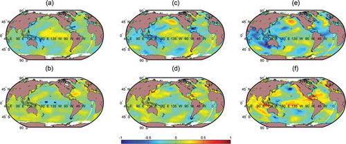
Of all the climate variables, the SST fields provide maximum information in terms of mirroring features during dry and wet events. Figure 2(c) and (d) shows the mean SST anomaly fields during events corresponding to SPAI-3 and SPAI-3, respectively. Several zones show opposite anomalies during the opposite precipitation extremes. The clarity of these opposite features is dependent on the temporal scale of study, as is evident from a comparison of Fig. 2(a), (c) and (e). Figure 2(a) shows the mean SST anomalies of dry events for SPAI-1, while Fig. 2(c) and (e) shows the same for SPAI-3 and SPAI-6, respectively. Similarly, Fig. 2(b), (d) and (f) shows the mean SST anomalies of wet events for SPAI-1, SPAI-3 and SPAI-6, respectively. The zones of opposite anomalies become larger and more well defined when the temporal scale is increased from 1-month to 6-months. However, since the core regions of opposite anomaly zones are of interest, a temporal scale of 3-months is adopted as the zones are sufficiently well defined at this scale.

Figure 2. Mean SST fields during dry (SPAI < −0.8) and wet (SPAI > 0.8) events, respectively, at (a) and (b) 1-month, (c) and (d) 3-month, (e) and (f) 6-month temporal scales. The range of the colourbar is fixed between 1 and −1 for ease of comparison. The zones with opposite features gradually improve with respect to their extent and crispness with the increase in the temporal scale of SPAI.

To appreciate the opposite features, the grid-wise differences in SST anomalies during dry and wet events are computed, and a map showing the global SST anomaly difference is constructed (Fig. 3). As mentioned earlier, only the core regions of the zones with statistically significant (99%) anomaly differences are considered. It is found that the anomaly differences in these core regions are statistically significant at as high as 99.9% confidence level (p-value is less than 0.001).

Figure 3. Differences in mean SST anomalies during dry events (SPAI-3 < −0.8) and wet events (SPAI-3 > 0.8) at 3-month temporal scale. Possible representative zones are shown in rectangles.

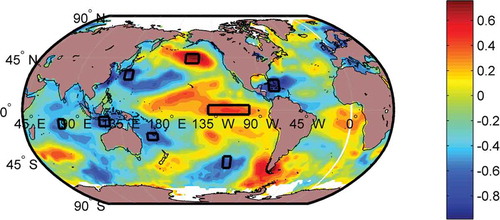
A large contiguous zone is identified in the equatorial Pacific Ocean, between 5°N–5°S and 100°W–140°W. This area is found to be a part of the Niño regions (between 5°N–5°S and 160°E–80°W), which are instrumental in influencing weather patterns globally. In fact, this region is approximately coincident with the Niño 3.4 regions (5°N–5°S and 120°W–170°W).

The anomaly differences in the North Pacific region (lying between 40°N–48°N and 150°W–165°W) are even stronger than those in the equatorial Pacific Ocean zones (Fig. 3). The location and the anomaly pattern of this zone are similar to those of the warm and cold phases of the PDO, having a time period of a few decades, typically 40–60 years. It may be possible that Indian dry and wet events are associated with a transitory circulation pattern of a smaller time period in the North Pacific. Three other zones in the Pacific Ocean (20°S–26°S and 160°E–170°E; 26°N–34°N, 136°E–144°E; 40°S–50°S, 114°W–124°W) are found to exhibit negative (positive) anomalies during the dry (wet) events in the target region. The cold anomalies in these zones may be attributed to the West Pacific SST Gradient (WPG), which is found to be strengthened since the 1980s (Hoell and Funk 2013). It can be speculated that warm anomalies in the equatorial east Pacific are not by themselves sufficient for triggering dry events. A particular pattern of cold anomalies along the west Pacific must coexist with warm anomalies along the east Pacific for dry extremes to occur in India. These anomalies may result from the low-frequency inter-annual to decadal west Pacific sea level and circulation changes attributed to the complex water exchange around the Philippine archipelago (Zhuang et al. 2013).

Negative anomalies are observed in the southern Indian Ocean (8°S–16°S and 74°E–80°E) and also to the northwest of Australia, i.e. the Timor Sea (6°S–14°S and 114°E–124°E). It may be observed from Figs 2 and 3 that, on an average, colder SST anomalies are observed in the southern and eastern Indian Ocean during dry events in the target area.

In the Atlantic Ocean, strong negative (positive) anomalies in the region (16°N–26°N and 70°W–80°W) between the North and South Americas are associated with dry (wet) events in India. The difference in anomalies is stronger towards the western part of the Atlantic Ocean, a little to the left of the zone responsible for the Atlantic Multidecadal Oscillation (AMO). Thus, as many as eight representative SST zones (Fig. 3), distributed across the globe, are clearly discernible.

It may be noted that some of the selected zones highlight the already established teleconnection patterns. They reaffirm previous findings such as the role of SSTs in the Pacific Ocean and Indian Ocean in influencing ISMR (Rasmusson and Carpenter 1983, Saji et al. 1999). Thus, the proposed approach is capable of identifying the previously known teleconnection patterns as well as other lesser known but potentially influential zones.

3.1.2 Global fields of surface pressure (SP) 

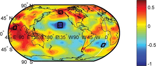
Surface pressure is found to be the second most interpretive climate variable that shows opposite anomaly patterns at a number of distinct zones during dry and wet extremes at the target area. The differences in anomalies are plotted in Figure 4. Similar to SST, the anomaly differences in the core regions are found to be statistically significant at 99.9% confidence level (p-value is less than 0.001). In the North Pacific (55°N–65°N and 145°W–160°W) positive (negative) anomalies are exhibited during dry (wet) events in the target region. In the tropical Pacific (15°N–30°N, 145°W–160°W), negative (positive) anomalies are observed during dry (wet) events in the target region. The whole of the Arabian Sea and Indian Ocean exhibit strong anomaly differences which are represented through a small area bounded by 10°N–20°N and 55°E–65°E. In the southern parts of the Atlantic Ocean (30°S–40°S, 0°–10°W), small negative anomalies are seen during dry events at the target region. Thus, four distinct zones (Fig. 4) are found to reflect opposite features in anomalies during dry and wet events.

Figure 4. Differences in mean SP anomalies during dry events (SPAI-3 < −0.8) and wet events (SPAI-3 > 0.8) at 3-month temporal scale. Possible representative zones are shown in rectangles.

3.1.3 Global fields of air temperature (AT), wind speed (WS), total precipitable water (TPW) and relative humidity (RH) 

The AT, WS, TPW and RH are generally known to influence convective activity on a smaller spatial scale rather than the planetary scale considered for the other climate variables such as SST and SP. Hence, we focus on the distinct zones in and around the study area. Figure 5 shows the local patterns of AT, WS and TPW which are explored for specific information. In the case of RH, the zones are found to be relatively poorer and less conspicuous (not shown in figures) than observed in the case of TPW. As the TPW and RH are closely related, RH was not considered separately after already considering TPW.

Figure 5. Differences in mean anomalies during dry (SPAI-3 < −0.8) and wet events (SPAI-3 > 0.8) at 3-month temporal scale for (a) AT (b) WS and (c) TPW. Possible representative zones are shown in rectangles.

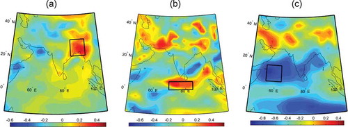
Warm anomalies of AT over the nook of the Bay of Bengal (20°N–30°N and 85°E–95°E) and very strong negative TPW anomalies around the Persian Gulf (5°N–15°N and 55°E–65°E) are found to be associated with dry events in the target region. Positive (negative) WS anomalies in the Indian Ocean (0°–5°N, 70°E–85°E) are found to be consistent during dry (wet) events in the target region. Thus, a period of high temperature and wind activity, along with insufficient precipitable water around the subcontinental region make up the ideal local climatic configuration heralding dry events in the Indian mainland. It is worthwhile to note here that the areal extent of the selected WS anomaly zone resembles the EQUINOO zone very closely; once again pointing to the fact that established teleconnection patterns are highlighted through the proposed approach for identification of GCP.

Summarizing the aforementioned findings, 15 zones are identified to characterize the GCP. These zones (summarized in Table 1) show significantly contrasting features, causing dry and wet precipitation extremes of Indian rainfall. It can be reiterated that the physical justification for some of the identified regions reaffirms the previously established hydroclimatic teleconnections. However, it is established that regional precipitation extremes at a relatively smaller spatial scale (continental scale) are linked to extensive GCP, rather than only a few preselected oceanic–atmospheric patterns. Though the physical justification for some of the zones is speculative, nonetheless it indicates and possibly completes the extensive climate signal pool from all across the globe. It may be worth noting that this pattern is, of course, specific to the target region and the considered hydrological event at the target region. If the target region is altered, a different GCP is expected to emerge. Moreover, even for the same target area, if a large-scale change in land use–land cover (LULC) occurs, then caution should be exercised before using the identified GCP. The occurrence of continental-scale changes in LULC is a rather slow process and is not expected to happen suddenly. Such changes would affect the continental-scale hydrological cycle, thereby altering the precipitation regime, nature of monsoon, etc. This would, in turn, affect the location and extent of the identified GCP. Hence, it is recommended to check the identified zones and revise them accordingly if significant change in large-scale LULC is suspected for the target area. It may be noted that, for our study area, no major changes in large-scale LULC and precipitation regime were observed during the study period.

Table 1. Identified representative zones of climate anomalies to characterize the GCP that are used to assess the possibility of classification of dry and wet events based on global climate fields.

Physical variable	Symbol	Latitude	Longitude
Air temperature	AT	20°N–30°N	85°E–95°E
Wind speed	WS	0°–5°N	70°E–85°E
Total precipitable water	TPW	5°N–15°N	55°E–65°E
Surface pressure	SP1	15°N–30°N	145°W–160°W
Surface pressure	SP2	30°S–40°S	0°–10°W
Surface pressure	SP3	55°N–65°N	145°W–160°W
Surface pressure	SP4	10°N–20°N	55°E–65°E
Sea surface temperature	SST1	40°N–48°N	150°W and 164°W
Sea surface temperature	SST2	16°N–26°N	70°W–80°W
Sea surface temperature	SST3	20°S–26°S	160°E–170°E
Sea surface temperature	SST4	4°N and 4°S	100°W and 140°W
Sea surface temperature	SST5	8°S and 16°S	74°E and 80°E
Sea surface temperature	SST6	6°S–14°S	114°E–124°E
Sea surface temperature	SST7	40°S–50°S	116°W–124°W
Sea surface temperature	SST8	26°N–34°N	136°E–144°E

Further, it may be noted that reliable identification of GCP is dependent on the correctness of the data used. The precipitation dataset used in this study has undergone sufficient quality checks. Minor changes in the precipitation dataset are not expected to have much effect on the GCP as long as the extreme events are identified correctly. There might be some changes in the boundaries of the identified zones with contrasting features. Hence, as mentioned earlier, it is recommended that the core regions of the statistically significant zones be selected. Then the identified GCP is expected to remain unchanged for the target area. However, if data for a particular target region are known to be highly uncertain, then it is recommended that some initial quality check and data pre-processing be performed before applying the proposed approach.

3.2 Potential of the GCP

3.2.1 Prediction of precipitation events using identified GCP 

As mentioned earlier, the dimensionality reduction of the n-dimensional input (n = 15) is obtained by performing PCA. The number of principal components (n_c) to be considered must serve two criteria: (i) it should be large enough to incorporate maximum information hidden in the identified GCP, and (ii) it should not be too large to hamper the SVM training owing to the curse of dimensionality. The entire analysis, comprising all the modelling steps, is repeated 15 times, varying the number of considered principal components (n_c) from 1 to 15. The value of contingency coefficient (C) is used to arrive at the optimum value of n_c. It is found that the value of C during the testing period is highest (indicating best performance) (Fig. 6) when the first six principal components are considered.

Figure 6. Variation of contingency coefficient C with number of principal components during testing period (2001–2010).

The selected principal components of the GCP are subjected to SVM training and classification as described in Section 2.4.2. The performance is assessed by inspecting the contingency table (Table 2(a)). It is found that for both development and testing periods, many of the events are predicted correctly. The performance is quantitatively evaluated through C, which was explained earlier. The value of C is obtained as 0.295 and 0.546 during the model development and testing periods, respectively. The considerably higher value of C obtained during the testing period (as compared to the development period) may be explained by the fact that it corresponds to the best performance possible during the testing period, which was used as a criterion for deciding upon the number of principal components to be considered in the analysis.

Table 2. Contingency table for multi-class classification using identified GCP and previous KV.

	Development period (1959–2000)			Testing period (2001–2010)
Observed category	Predicted category
	Dry	Normal	Wet	Dry	Normal	Wet
(a) GCP
Dry	53	5	17	12	1	5
Normal	122	39	140	5	3	66
Wet	22	11	68	0	3	20
Q	45.400			48.865
	4			4
p-value
C	0.295			0.546
	0.817			0.817
	0.361			0.668
(b) KV
Dry	47	6	26	1	0	18
Normal	137	29	148	4	2	71
Wet	31	7	73	0	2	22
Q	22.632			3.821
	4			4
p-value
C	0.207			0.176
	0.817			0.817
	0.253			0.215

3.2.2 Comparison of GCP potential with respect to previously known indicators 

The location of the 15 variables comprising the GCP was explained in Section 3.1. It may be noted that out of the eight identified SST zones, the one lying in the equatorial Pacific Ocean (SST4, Table 1) resembles the Nino 3.4 zone very closely. Again, another identified SST zone (SST5, Table 1), though it does not coincide with the poles of IOD, definitely bears the signature of the Indian Ocean SSTs. It is an established fact that the SSTs in the equatorial Pacific Ocean and equatorial Indian Ocean have an important role in influencing ISMR (Clark et al. 2000, Maity and Nagesh Kumar 2006, Rajagopalan and Molnar 2012). Thus, the proposed approach is capable of identifying the teleconnection patterns that have been previously discovered and established to be instrumental for ISMR anomalies, besides bringing forth new zones of importance. Hence, the two variables mentioned immediately above are together designated as the known variables (KV), which represent the well-known indicators of ISMR. In this section, a comparison of the potential of GCP with that of KV in predicting extremes of Indian rainfall is presented.

For this purpose, the prediction process is repeated using KV in place of GCP. Reduction of dimensionality is not required here, since the KV consists of only two variables. Still the PCA is performed for statistical uniformity and both the principal components are considered for the subsequent SVM training and prediction. The values of C during model development and testing periods are found to be 0.207 and 0.176, respectively. The complete contingency table is shown in Table 2(b). Comparing the Tables 2(a) and 2(b), it may be safely concluded that a higher degree of association between observed and predicted categories is achieved using the proposed GCP as against the KV. Next, we look at individual extreme events that were observed during the testing period. In the year 2002, the monsoon failed and droughts were observed for each of the 3-month periods of May–June–July (MJJ), June–July–August (JJA), July–August–September (JAS), August–September–October (ASO) and September–October–November (SON). In the case of GCP, these periods are predicted to be dry (SPAI ; whereas in the case of KV, these periods are predicted as wet (SPAI. Hence, while the former correctly predicts five out of the five dry events in 2002, the latter predicts none. Similarly, all the three dry events of 2009 are also correctly predicted to be dry when the principal components of the GCP are used as model input, but all are incorrectly predicted as wet events when the principal components of the KV are used. Thus, the information obtained from the extensive GCP, when processed properly, has remarkable merits over the few traditionally used teleconnection patterns in predicting precipitation extremes.

4 Summary and conclusions

The findings of this study establish the existence of a specific global climate pattern behind hydrological extremes observed at a relatively small spatial scale. The GCP is characterized by a set of different climate variables from different, distinct zones on the globe. The study reveals the fact that assessment of the long recognized hydroclimatic teleconnection of one or two specific and predetermined large-scale circulation pattern(s) may not necessarily be exhaustive for a comprehensive analysis of regional precipitation extremes. A number of zones of opposite anomalies are obtained for six climate variables during dry and wet events at the target area. Among the climate variables, SST and SP anomaly zones are found to be widely distributed over the globe and the source of maximum hydroclimatic information. Other variables such as AT, WS and TPW are considered on a smaller spatial scale. The distinct climate anomaly maps responsible for dry and wet events at the target area confirm the existence of specific globally extended climate patterns, apart from reaffirming the already known hydroclimatic teleconnections for Indian rainfall, such as ENSO or IOD or both. The proposed GCP, comprising 15 identified indicator variables, is subjected to PCA analysis and the first six principal components are used as inputs to two binary SVM models simultaneously. Their outputs are logically combined to obtain the predicted categories of all precipitation events. A similar prediction exercise is undertaken with the KV, which denote the known indicators of ISMR. The prediction performances are then compared and it is found that the former provides a more robust prediction of precipitation events at the target area compared to the latter. Thus, the proposed approach may be substantially useful in explaining apparent paradoxes in extreme precipitation behaviour on a continental scale. Moreover, future research work may be carried out to explore the possibility of extending the methodology to extremes of other hydrological variables such as soil moisture, runoff, etc.

Since the proposed approach of identifying the GCP is a generalized approach, it may be extended to other target areas across the world. However, it is expected that the minimum spatial scale of the target area required to identify a reliable GCP would vary based on the geographical location of the target area. In general, as the spatial extent of the target area is reduced, the global hydroclimatically influential zones would become less conspicuous. For instance, extreme events occurring in a small basin may be triggered by many local factors rather than systematic large-scale global circulation patterns. For a small target area, the global anomaly zones (of contrasting features) may not be very reliable. They may be scattered, less numerous and inconclusive. In the absence of large contiguous zones of contrasting features (during opposite extremes), the core regions would be difficult to select and thus identification of GCP would be difficult. However, the proposed methodology may be replicated with other target areas of similar spatial extent as that of India. Even smaller spatial scales may be used, but it is preferable not to apply the methodology on target areas less than approximately 10⁵ km². This may be treated as a rough guideline only. It is recommended to investigate whether contiguous zones of contrasting features are identifiable for potential use as GCP for any given target area.

Acknowledgements

Monthly Indian precipitation data were obtained from the India Meteorological Department (IMD) for the period 1959–2010. Monthly gridded climate data (Reanalysis I) for six global climate variables were obtained from the National Oceanic and Atmospheric Administration (NOAA) (http://www.esrl.noaa.gov/psd/data/gridded/data.ncep.reanalysis.surface.html) for the period 1958–2010. The authors would like to acknowledge the data providers.

Disclosure statement

No potential conflict of interest was reported by the authors.

Additional information

Funding

The authors acknowledge the partial financial support from a research project sponsored by the Ministry of Earth Science (MoES), Government of India (Sanction order# MoES/PAMC/H&C/30/2013-PC-II).

References

- Abram, N.J., et al., 2007. Seasonal characteristics of the Indian Ocean Dipole during the Holocene epoch. Nature, 445, 299–302. doi:10.1038/nature05477
- Anirudh, V. and Umes, C.K., 2007. Classification of rainy days using SVM. Norfolk, Virginia: Proceedings of Symposium at HYDRO.
- Bhagwat, P.P. and Maity, R., 2012. Multistep-ahead river flow prediction using LS-SVR at daily scale. Journal of Water Resource and Protection, 4, 528–539. doi:10.4236/jwarp.2012.47062
- Boser, B.E., Guyon, I., and Vapnik, V., 1992. A training algorithm for optimal margin classifiers. Proceedings Fifth annual Workshop on Computational Learning Theory, Pittsburgh, 144–152. doi:10.1145/130385.130401
- Brandimarte, L., et al., 2011. Relation between the north-atlantic oscillation and hydroclimatic conditions in mediterranean areas. Water Resources Management, 25 (5), 1269–1279. doi:10.1007/s11269-010-9742-5
- Bray, M. and Han, D., 2004. Identification of support vector machines for runoff modelling. Journal of Hydroinformatics, 6, 265–280.
- Cai, W. and Vanrensch, P., 2012. The 2011 southeast Queensland extreme summer rainfall: a confirmation of a negative pacific decadal oscillation phase? Geophysical Research Letters, 39, L08702. doi:10.1029/2011GL050820
- Chen, H., et al., 2010. Downscaling GCMs using the smooth support vectormachine method to predict daily precipitation in the Hanjiang basin. Advances in Atmospheric Science, 27 (2), 274–284. http://dx.doi.org/10.1007/s00376-009-8071-1
- Chiew, F.H.S. and McMahon, T.A., 2002. Global ENSO-streamflow teleconnection, streamflow forecasting and interannual variability. Hydrological Sciences Journal, 47 (3), 505–522. doi:10.1080/02626660209492950
- Clark, C.O., Cole, J.E., and Webster, P.J., 2000. Indian ocean SST and Indian summer rainfall: predictive relationships and their decadal variability. Journal of Climate, 13, 2503–2519. doi:10.1175/1520-0442(2000)013<2503:IOSAIS>2.0.CO;2
- Cristianini, N. and Shawe-Taylor, J., 2000. An introduction to support vector machines: and other kernel-based learning methods. Cambridge: Cambridge University Press.
- Feng, S. and Hu, Q., 2008. How the North Atlantic Multidecadal Oscillation may have influenced the Indian summer monsoon during the past two millennia. Geophysical Research Letters, 35, L01707. doi:10.1029/2007GL032484
- Francis, P.A. and Gadgil, S., 2013. A note on new indices for the equatorial Indian Ocean oscillation. The Journal of Earth System Science, 122 (4), 1005–1011. doi:10.1007/s12040-013-0320-0
- Fu, G., et al., 2013. Temporal variation of extreme rainfall events in China. 1961–2009. Journal of Hydrology, 487, 48–59. doi:10.1016/j.jhydrol.2013.02.021
- Gadgil, S., et al., 2004. Extremes of the Indian summer monsoon rainfall, ENSO and equatorial Indian Ocean oscillation. Geophysical Research Letters, 31, L12213. doi:10.1029/2004GL019733
- Giannini, A., Biasutti, M., and Verstraete, M.M., 2008. A climate model-based review of drought in the Sahel: desertification, the re-greening and climate change. Global and Planetary Change, 64, 119–128. doi:10.1016/j.gloplacha.2008.05.004
- Gibbons, J.D. and Chakraborti, S., 2011. Nonparametric statistical inference. 5th ed. Boca Raton, FL: Chapman and Hall.
- Goswami, B.N., et al., 2006. A physical mechanism for North Atlantic SST influence on the Indian summer monsoon. Geophysical Research Letters, 33, L02706. doi:10.1029/2005GL024803
- Gu, W., et al., 2009. Interdecadal unstationary relationship between NAO and east China’s summer precipitation patterns. Geophysical Research Letters, 36, L13702. doi:10.1029/2009GL038843
- Guyon, I., Boser, B., and Vapnik, V., 1993. Automatic capacity tuning of very large VC-dimension classifiers. In: H.S. José, C. Jd, and G.C. Lee, eds. Advances in neural information processing systems. Vol. 5. San Mateo: Morgan Kaufmann, 147–155.
- Hoell, A. and Funk, C., 2013. The ENSO-Related West Pacific Sea surface temperature gradient. Journal of Climate, 26, 9545–9562. doi:10.1175/JCLI-D-12-00344.1
- Hoerling, M., 2003. The perfect ocean for drought. Science, 299 (5607), 691–694. doi:10.1126/science.1079053
- Jiang, P., et al., 2013. How well do the GCMs/RCMs capture the multi-scale temporal variability of precipitation in the Southwestern United States? Journal of Hydrology, 479, 75–85. doi:10.1016/j.jhydrol.2012.11.041
- Jolliffe, I.T., 1986. Principal component analysis. New York, NY: Springer.
- King, A.D., Alexander, L.V., and Donat, M.G., 2013. Asymmetry in the response of eastern Australia extreme rainfall to low-frequency Pacific variability. Geophysical Research Letters, 40, 2271–2277. doi:10.1002/grl.50427
- Kişi, O. and Çimen, M., 2009. Evapotranspiration modelling using support vector machines / Modélisation de l’évapotranspiration à l’aide de ‘support vector machines’. Hydrological Sciences Journal, 54 (5), 918–928. doi:10.1623/hysj.54.5.918
- Kousky, V.E., Kagano, M.T., and Cavalcanti, I.F.A., 1984. A review of the Southern Oscillation: oceanic-atmospheric circulation changes and related rainfall anomalies. Tellus, 36A (5), 490–504. doi:10.1111/j.1600-0870.1984.tb00264.x
- Krishna Kumar, K., 1999. On the weakening relationship between the Indian monsoon and ENSO. Science, 284, 2156–2159. doi:10.1126/science.284.5423.2156
- Krishnamurthy, L. and Krishnamurthy, V., 2013. Decadal scale oscillations and trend in the Indian monsoon rainfall. Climate Dynamics. doi:10.1007/s00382-013-1870-1
- Li, S., et al., 2008. Modelling the influence of North Atlantic multidecadal warmth on the Indian summer rainfall. Geophysical Research Letters, 35, L05804. doi:10.1029/2007GL032901
- Lin, J.-Y., Cheng, C.-T., and Chau, K.-W., 2006. Using support vector machines for long-term discharge prediction. Hydrological Sciences Journal, 51 (4), 599–612. doi:10.1623/hysj.51.4.599
- Maity, R., Bhagwat, P.P., and Bhatnagar, A., 2010. Potential of support vector regression for prediction of monthly streamflow using endogenous property. Hydrological Processes, 24, 917–923. doi:10.1002/hyp.7535
- Maity, R. and Kashid, S.S., 2010. Short-term basin-scale streamflow forecasting using large-scale coupled atmospheric oceanic circulation and local outgoing longwave radiation. Journal of Hydrometeorology, American Meteorological Society (AMetSoc), 11 (2), 370–387. doi:10.1175/2009JHM1171.1
- Maity, R. and Kashid, S.S., 2011. Importance analysis of local and global climate inputs for basin-scale streamflow prediction. Water Resources Research, American Geophysical Union, 47, W11504. doi:10.1029/2010WR009742
- Maity, R. and Nagesh Kumar, D., 2006. Hydroclimatic association of the monthly summer monsoon rainfall over India with large-scale atmospheric circulations from tropical Pacific Ocean and the Indian Ocean region. Atmospheric Science Letters, 7, 101–107. doi:10.1002/asl.141
- Maity, R. and Nagesh Kumar, D., 2008. Basin-scale stream-flow forecasting using the information of large-scale atmospheric circulation phenomena. Hydrological Processes, 22 (5), 643–650. doi:10.1002/hyp.6630
- Maity, R., Ramadas, M., and Govindaraju, R.S., 2013. Identification of hydrologic drought triggers from hydroclimatic predictor variables. Water Resources Research, American Geophysical Union, 49, 4476–4492. doi:10.1002/wrcr.20346
- Mo, K.C. and Schemm, J.E., 2008. Relationships between ENSO and drought over the southeastern United States. Geophysical Research Letters, 35, L15701. doi:10.1029/2008GL034656
- Nicholls, N., 1983. Predicting Indian monsoon rainfall from sea-surface temperature in the Indonesia–north Australia area. Nature, 306, 576–577. doi:10.1038/306576a0
- Oubeidillah, A.A., Tootle, G., and Anderson, S.-R., 2012. Atlantic Ocean sea-surface temperatures and regional streamflow variability in the Adour-Garonne basin, France. Hydrological Sciences Journal, 57 (3), 496–506. doi:10.1080/02626667.2012.659250
- Panda, D.K., et al., 2013. Streamflow trends in the Mahanadi River basin (India): linkages to tropical climate variability. Journal of Hydrology, 495, 135–149. doi:10.1016/j.jhydrol.2013.04.054
- Parthasarathy, B., Munot, A.A., and Kothaale, D.R., 1995. All-India monthly and seasonal rainfall series: 1871–1993. Theoritical and Applied Climatology, 49, 217–224. doi:10.1007/BF00867461
- Pearson, K., 1904. On the theory of contingency and its relation to association and normal correlation. Draper’s Comp. Res. Mem. Biometric Ser. I, London, UK: Dulau and Co.
- Philipp, A., et al., 2007. Long-term variability of daily North Atlantic–European pressure patterns since 1850 classified by simulated annealing clustering. Journal of Climate, 20, 4065–4095. doi:10.1175/JCLI4175.1
- Qin, Z., et al., 2005. Application of least squares vector machines in modelling water vapor and carbon dioxide fluxes over a cropland. Journal of Zhejiang University Science, 6B (6), 491–495. doi:10.1631/jzus.2005.B0491
- Qiu, Y., et al., 2014. The asymmetric influence of the positive and negative IOD events on China’s rainfall. Scientific Reports, 4, 4943. doi:10.1038/srep04943
- Raghavendra, N.S. and Deka, P.C., 2014. Support vector machine applications in the field of hydrology: a review. Applied Soft Computing, 19, 372–386. http://dx.doi.org/10.1016/j.asoc.2014.02.002
- Rajagopalan, B. and Molnar, P., 2012. Pacific Ocean sea-surface temperature variability and predictability of rainfall in the early and late parts of the Indian summer monsoon season. Climate Dynamics, 39 (6), 1543–1557. doi:10.1007/s00382-011-1194-y
- Rajeevan, M., et al., 2006. High resolution daily gridded rainfall data for the Indian region: analysis of break and active monsoon spells. Current Science, 91 (3), 296–306.
- Rasmusson, E.M. and Carpenter, T.H., 1983. The relationship between eastern equatorial Pacific sea surface temperature and rainfall over India and Sri Lanka. Monthly Weather Review, 111, 517–528. doi:10.1175/1520-0493(1983)111<0517:TRBEEP>2.0.CO;2
- Rogers, J.C., 2013. The 20th century cooling trend over the southeastern United States. Climate Dynamics, 40 (1–2), 341–352. doi:10.1007/s00382-012-1437-6
- Saji, N.H., et al., 1999. A dipole mode in the tropical Indian Ocean. Nature, 401, 360–363. doi:10.1038/43854
- Samsudin, R., Saad, P., and Shabri, A., 2011. River flow time series using least squares support vector machines. Hydrology and Earth System Sciences, 15, 1835–1852. doi:10.5194/hess-15-1835-2011
- She, N. and Basketfield, D., 2005. Long range forecast of streamflow using support vector machine. In: R. Walton ed. Proceedings of the world water and environment resources congress ASCE, May 15–19, 2005, Anchorage: Alaska. doi:10.1061/40792(173)481
- Shelton, M.L., 2009. Hydroclimatology: perspectives and applications. New York: Cambridge University Press.
- Singhrattna, N., Babel, M.S., and Perret, S.R., 2012. Hydroclimate variability and long-lead forecasting of rainfall over Thailand by large-scale atmospheric variables. Hydrological Sciences Journal, 57 (1), 26–41. doi:10.1080/02626667.2011.633916
- Terray, P., et al., 2003. Sea surface temperature associations with the late Indian summer monsoon. Climate Dynamics, 21, 593–618. doi:10.1007/s00382-003-0354-0
- Ting, M., et al., 2011. Robust features of Atlantic multi-decadal variability and its climate impacts. Geophysical Research Letters, 38, L17705. doi:10.1029/2011GL048712
- Tripathi, S.H., Srinivas, V.V., and Nanjundiah, R.S., 2006. Downscaling of precipitation for climate change scenarios: a support vector machine approach. Journal of Hydrology, 330, 621–640. doi:10.1016/j.jhydrol.2006.04.030
- Vapnik, V.N., 1998. Statistical learning theory. New York, NY: John Wiley & Sons.
- Viswambharan, N. and Mohanakumar, K., 2014. Modulation of Indian summer monsoon through northern and southern hemispheric extra-tropical oscillations. Climate Dynamics, Springer, Article in press, 43, 925–938. doi:10.1007/s00382-014-2049-0
- Wang, B., et al., 2013. Northern Hemisphere summer monsoon intensified by mega-El Niño/southern oscillation and Atlantic multidecadal oscillation. Proceedings of the National Academy of Sciences of the United States of America. doi:10.1073/pnas.1219405110
- Willems, P., 2013. Multidecadal oscillatory behaviour of rainfall extremes in Europe. Climatic Change, 120 (4), 931–944. doi:10.1007/s10584-013-0837-x
- Wong, W.K., et al., 2011. Climate change effects on spatiotemporal patterns of hydroclimatological summer droughts in Norway. Journal of Hydrometeorology, 12 (6), 1205–1220. doi:10.1175/2011JHM1357.1
- Wu, R. and Zhang, L., 2010. Biennial relationship of rainfall variability between Central America and equatorial South America. Geophysical Research Letters, 37, L08701. doi:10.1029/2010GL042732
- Ye, J.-S., 2014. Trend and variability of China’s summer precipitation during 1955–2008. International Journal of Climatology, 34, 559–566. doi:10.1002/joc.3705
- Yuan, X. and Wood, E.F., 2013. Multimodel seasonal forecasting of global drought onset. Geophysical Research Letters, 40. doi:10.1002/grl.50949
- Zakaria, Z.A. and Shabri, A., 2012. Streamflow forecasting at ungaged sites using support vector machines. Applied Mathematical Sciences, 6 (60), 3003–3014.
- Zhuang, W., Qiu, B., and Du, Y., 2013. Low-frequency western Pacific Ocean sea level and circulation changes due to the connectivity of the Philippine Archipelago. Journal of Geophysical Research Oceans, 118, 6759–6773. doi:10.1002/2013JC009376