
ABSTRACT
Forecasting future water demands has always been of great complexity, especially in the case of tourist cities which are subject to population fluctuations. In addition to the usual uncertainties related to climate and weather variables, daily water consumption in Mashhad, a tourist city is affected by a significant different fluctuation. Mashhad is the second most populous city in Iran. The number of tourists visiting the city is subject to national and religious events, which are respectively based on the Iranian formal calendar (secular calendar) and the Arabic Hijri calendar (Islamic religious calendar). Since religious events move relative to the secular calendar, the coincidence of the two calendars results in peculiar wild fluctuations in population. Artificial neural networks (ANNs) are chosen to predict water demand under such conditions. Three types of ANNs, feedforward back-propagation, cascade-forward and radial basis functions, are developed. In order to track how population fluctuation propagates in the model and affects the outputs, two sets of inputs are considered. For the first set, based on evaluating several repetitions, a typical combination of variables is selected as inputs, whereas for the second set, new calendar-based variables are included to decrease the effect of population fluctuations; the results are then compared using some performance criteria. A large number of runs are also conducted to assess the impact of random initialization of the weights and biases of networks and also the effect of calendar-based inputs on improvement of network performance. It is shown that, from the points of view of performance measures and unchanging outputs through numerous runs, the radial basis network that is trained by patterns including calendar-based inputs can provide the best domestic water demand forecasting under population fluctuations.
Editor D. Koutsoyiannis Associate editor E. Rozos
1 Introduction
Water resources planning and management is greatly influenced by estimation of future water demands. Long-term water demand forecasting is essential for design of water resources structures, whereas short-term forecasting is needed for reservoir operation and management of water transmission and distribution facilities such as pumping stations and pipe networks (Yurdusev and Firat Citation2009). While complexity of municipal water demand forecasting justifies employing nonlinear information processing systems, other demands such as agricultural, environmental and industrial demands are usually estimated by means of empirical equations (Felfelani et al. Citation2013). According to literature on the subject, several researchers have addressed urban water consumption forecasting not only by means of various methodologies but also by using different combinations of inputs such as population, climatic and weather conditions, the day of the week, socio-economic factors and cultural behaviour of societies. These factors have not been considered eligible as inputs for models in all research. Some studies considered climatic factors such as temperature and precipitation as significant variables (e.g. Billings and Agthe Citation1998, Zhou et al. Citation2000), while others focused on historical demand observations, and claimed that the effect of climatic variables is reflected directly in the consumption time series, and therefore these variables do not need to be separately included as inputs (e.g. Jowitt and Xu Citation1992). Homwongs et al. (Citation1994) presented an adaptive smoothing–filtering approach for on-line forecasting of hourly municipal water use time series. They showed that the forecasting system can maintain surprisingly small forecasting errors, despite various unmodelled time-varying climatic variability. Zhang et al. (Citation2006) claimed that in the winter season climate factors have little effect on domestic water demands. Therefore, they used only historical demand as the input. In the summer season, the difference between weekday and weekend demands and climate factors such as temperature, relative humidity, dew point, wind speed and rainfall were incorporated in their ANN models. They showed that their ANN models demonstrate strong capability in extracting the nonlinear relations between water demand and climatic variables. Ghiassi et al. (Citation2008) developed a dynamic ANN model for comprehensive urban water demand forecasting and demonstrated that, by using water demand time series, this kind of model can provide forecasts without explicit inclusion of weather factors. Firat et al. (Citation2009, Citation2010) used two types of fuzzy inference systems (an adaptive neuro-fuzzy inference system and a Mamdani fuzzy inference system) and also evaluated three schemes of neural networks to predict monthly water consumption. They developed six models with different input datasets. In these studies, input data were selected only from water consumption time series and other effective variables such as climatic factors were not considered. Herrera et al. (Citation2010) compared the efficiency of a series of alternative machine-learning methods for forecasting hourly water demand for a city in southeastern Spain. They assessed the efficacy of ANNs, projection pursuit regression, multivariate adaptive regression splines, random forests and support vector regression in domestic water demand forecasting. In the referenced paper, in addition to water demand time series, weather time series, temperature, wind velocity, atmospheric pressure, rain and the day of the week were also entered into the models. In recent research, hybrid models have been employed as time series forecasting tools. Campisi-Pinto et al. (Citation2012) tackled the problem of water demand forecasting by means of back-propagation ANNs coupled with wavelet denoising and used a 7-year time series of water demands as predictors.
In usual domestic demand forecasting cases, fluctuations of population are not taken into account. However, in cities such as Mashhad in Iran, where tourists have religious reasons for visiting the city, there is a peculiar fluctuation in population caused by the distribution of religious events and holidays in the calendar. The secular calendar, which is the solar type (like the Christian calendar), measures the time taken by the Earth to rotate around the Sun, while the lunar calendar is based on the amount of time it takes the Moon to move through all of its phases. Twelve lunar months are equal to 354.4 days, whereas the solar year is 365.2 days. So the lunar calendar (Islamic religious calendar) is shorter than the solar calendar (secular calendar) by about 11 days a year or 1 year in every 33 years. Therefore, the dates of religious events are not constant based on the solar calendar. The coincidence of religious events and weekends leads to a significant increase in the city’s population and water demand. This peculiar fluctuation in population can complicate the domestic water demand forecasting problem.
According to the literature on urban water demand forecasting, ANN models have performed very well in comparison with conventional regression models and other soft computing techniques. They are specifically of great interest for short-term forecasting while econometric models, coupled with simulation or scenario-based forecasting, are more likely to be used in long-term forecasting (Donker et al. Citation2014). Although a wide variety of ANN models have attracted attention, none evaluated the effect of peculiar fluctuations such as in population, and also none entered the calendar as an input to the ANN model. Therefore, in this paper, a comprehensive introduction to the real case of Mashhad city in Iran is presented. Three types of ANN models are developed using different classes of inputs and verified by use of two common performance criteria. Numerous runs are conducted to address the impact of random initialization of networks and also evaluate the effect of adding new calendar-based inputs on performance improvement. Finally, from the points of view of performance measures and unchanging outputs through runs, the best model is selected for the purpose of forecasting water consumption for the next 14 days.
2 Study area
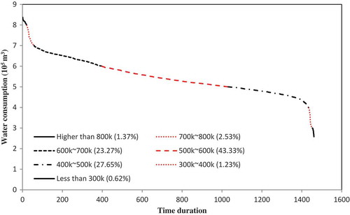
Mashhad is a city in the northeast of Iran with a cold and semi-arid climate. The mausoleum of Imam Reza, the eighth Imam of Shia Islam, is located in this city. The existence of the Imam Reza holy shrine makes Mashhad the centre of religious tourism in Iran. Its resident population of 3 million alongside more than 20 million annual visitors make it a huge water consumer. About 220 million cubic metres of water are needed to satisfy the annual domestic demand of the city. Daily water consumption in Mashhad varies considerably from 270 000 to 830 000 m3 during a year (). A load duration curve (LDC) for daily water consumption in Mashhad is shown in . About 94% of the observed data are between and
, while 6% of observations represent the extreme conditions (minimum and maximum consumption) which are hard to predict ().
Figure 1. Daily water consumption time series for Mashhad between March 2009 and July 2013. The time series includes a wide range of values from 270 000 to 830 000 m3 over a year. Dashed line shows the linear trend of demand time series. Ovals show some extreme effects of the coincidence of the two calendars that result in jumps (each represents a special religious holiday) in daily water consumption.
Figure 2. Load duration curve of Mashhad daily water consumption showing the approximate frequency of each value in the time series. The proportion of each class is inserted in the legend.
3 Artificial neural networks (ANNs)
Artificial neural network models are a class of flexible nonlinear information processing systems that are capable of machine learning, pattern recognition, function approximation and also forecasting. Mathematical generalization of neural biology, ANN model development and regulation, adjustment of the training algorithm and evaluation of the network performance are the cyclic steps that should be taken until an acceptable error rate is achieved (Fausett Citation1994). The trained network is then used to predict future values. Three types of neural networks, namely the common feedforward multi-layer perceptron with back-propagation algorithm (MLP-BP), cascade-forward (CF-BP) and radial basis functions (RBF), are evaluated in this study.
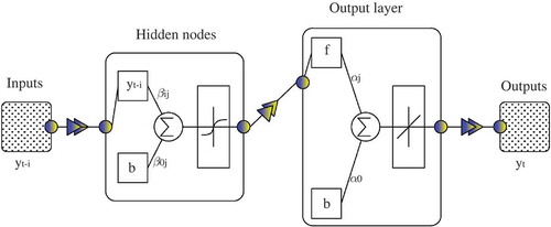
Figure 3. Schematic architecture of a feedforward multilayer perceptron with one hidden layer. A sigmoid activation function is used for the hidden layers and a linear activation function is assigned to the output node.
3.1 Multilayer perceptron with the back-propagation algorithm (MLP-BP)
Among many types of neural networks, the most popular one that is still of interest among researchers is the feedforward MLP. A typical MLP network comprises an input layer, at least one middle layer (or hidden layer) and an output layer (). The training process of the MLP network occurs through a back-propagation algorithm. The algorithm minimizes a quadratic error between the actual values and network outputs until errors reach acceptable values. A typical one-hidden-layer MLP model can be expressed as (Zhang and Qi Citation2005):
where n represents the number of hidden nodes, m represents the number of input nodes, f is a sigmoid activation function such as the hyperbolic tangent sigmoid activation function: ;
is the weight vector from the hidden to output nodes in which
and
are weights from the input to hidden nodes in which
and
.
and
as biases are weights on links leading from the units (b in ) that are used in both hidden and output layers and have activation values equal to 1. Note that equation (1) and propose a linear activation function (g) for the output node, as desired for forecasting problems (Zhang and Qi Citation2005).
3.2 Cascade-forward back-propagation (CF-BP)
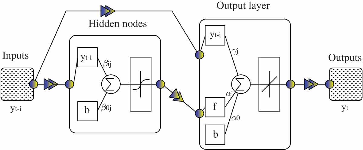
This network is very similar to feedforward MLP networks, but includes a weight connection from the input to each layer and also from each layer to the successive layers (). Therefore, the number of weight connections and biases in the cascade-forward network is greater compared to the MLP-BP network and this may lead to a slower training speed but a smaller required number of epochs (Hedayat et al. Citation2009). The cascade-forward network also resembles feedforward MLP in its use of a back-propagation training algorithm. In this work, the Levenberg-Marquardt training algorithm, which is known as the fastest back-propagation algorithm (Hagan et al. Citation1996), is used for both MLP and cascade-forward networks. Filik and Kurban (Citation2007) presented a new approach to short-term load forecasting using autoregressive (AR) analysis for the input of different ANN models, which were MLP-BP and CF-BP models. They found CF-BP to be more efficient. Therefore, in this study CF-BP is used and evaluated as an efficient approach to water consumption forecasting.
Figure 4. Schematic architecture of a cascade-forward network with one hidden layer. A sigmoid activation function for the hidden layers and a linear activation function for the output node are desired for forecasting problems.
3.3 Radial basis function networks (RBF)
In the context of neural networks, radial basis functions are functions only of the inputs’ distances from central points. A radial basis function neural network consists of two layers: the radial basis layer (or feature/kernels layer) and the linear layer ().
Figure 5. Schematic architecture of a typical radial basis network which has only two layers.
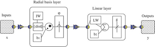
In , IW and LW are input weights and linear layer weights vectors, is the Euclidean distance between the input vector and IW (centres) and b is the bias vector. In most of the studies, the activation function in the radial basis layer is the Gaussian function radbas (equation (2)) and in the linear layer is a linear function (g).
where n is a function of the Euclidean norm. The output of a radial basis network can be written as:
where m is the number of centres, x is the input vector, b1 is the bias vector of the radial basis layer, b2 is the bias vector of the linear layer, .* is an operator that does element-by-element multiplication, and ϕi is the activation function, which is mostly a Gaussian function. In some manuscripts ϕi is referred to as the kernel (e.g. Giustolisi and Simeone Citation2006, Lin et al. Citation2006). In fact, kernel functions are used as a nonlinear mapping from the original space to a higher dimensional one in order to handle the nonlinear relationship and provide a more separable dataset.
In this research, Matlab® software and “newrb” syntax () are used to develop the radial basis network. In the syntax P and T are the input and output vectors,
is the acceptable mean square error (MSE),
is the spread index of radial basis functions. The determination of the
parameter is paramount in the model development process. If the value of
is very small, the number of training epochs increases and this would cause the overtraining condition (Tetko et al. Citation1995). So, in order to reach the optimum condition, the
parameter must be chosen near the minimum MSE value of the validation dataset. The determination of the optimum
parameter is also of great importance. Having small values of
makes the radbas functions sharper and decreases the overlapping intervals, and vice versa. As a general rule, if the function to be approximated is smooth, larger values for
will be selected, but for noisy and severely fluctuating functions, the
parameter must be small.
4 Input variables and data
In this research, to incorporate effects of population fluctuations, some new calendar-based inputs are considered in the water demand forecasting model. Regarding accessibility of data, input data are selected from 4-year daily water consumption time series, maximum and minimum air temperature, the day of the week, the day of the solar year and the day of the lunar year. Other climatic variables, such as humidity, that do not vary considerably in the study area are not considered. Several combinations of input data derived from a literature review are tested and total performance of the models evaluated using common criteria both in training and in testing progress. Finally, 26 variables in 10 categories are chosen as input vector of the ANNs (). Regarding the main scope of this study, which incorporates effects of population fluctuations by using some new calendar-based inputs, all ANN models are developed and evaluated considering two sets of inputs. For the first set of inputs, calendar-based variables (categories 2, 4–8 in ) are excluded from the training process, while for the second set, all 26 variables are taken into account. For each forecasting lead time, input data are arranged separately and according to the target day. For instance, if today is Monday 1 January, and we want to forecast the consumption 2 days from now, that is to say for Wednesday 3 January, the consumption of last Wednesday and also 3 January of the previous year are applied as the inputs; but if we want to forecast 5 days from now, that would be Saturday 6 January, the consumption of last Saturday and also 6 January a year before are considered as the inputs. Other variables such as calendar-based inputs are likewise arranged based on the target day. In this paper, to forecast daily water demands for the next 2 weeks, 14 data series are used as the inputs for 14 networks (each network for forecasting one lead time).
Table 1. Ten categories of input data to neural networks. Among these variables, ,
,
,
,
and
are the calendar-based inputs, which are used to consider effects of population fluctuations.
Networks that are trained by normalized and standardized data and patterns show better performance in convergence (Shanker et al. Citation1996, Luk et al. Citation2000, Aqil et al. Citation2007). Hence, the inputs are standardized by subtracting each column of the raw dataset () by its mean value (
) and dividing by the standard deviation (
) (equation (4)). Also to scale to be in the support domain of the activation functions (i.e.
), equation (5) is used.
where is the standardized dataset,
and
are the minimum and maximum values of the ith dataset and
is the normalized dataset.
5 Performance assessment
All the data series are divided into two groups randomly. Ninety percent of the data are selected as a training dataset to train the networks and 10% are chosen as a validation/test dataset to verify the model outputs. The training dataset is used in the training process and then the statistical criteria, regression coefficient and mean square error are calculated to assess the performance of the network by using the validation dataset which has not been involved in the training process:
where MSE and R respectively denote mean square error and regression coefficient, and
are the model outputs and observed data,
and
are the average values, and
is the number of data.
6 Results and discussion
The best configuration of neural networks is often determined by trial and error. So, through a trial and error process on over 2800 arrangements (networks with one to four hidden layers and with one to seven neurons in each layer), the best architectures for MLP-BP and CF-BP networks have been determined. A MLP-BP network with one hidden layer which has one neuron and a four-hidden-layer CF-BP network with 3-6-1-4 neurons in the hidden layers have the best performance. The training and simulation times of MLP-BP, CF-BP and RBF models (for 14 forecasting lead times) are about 2, 5 and 4 minutes, respectively. The MSE and R indices calculated using the validation dataset show the performance of both MLP-BP and CF-BP models in forecasting water consumption 1–14 days ahead (). The average values of R and MSE for 14 MLP-BP networks (14 networks for water demand forecasting in different daily lead times) are 0.8338 and 0.0291, while for CF-BP networks these values are 0.864 and 0.0263 ().
Table 2. Values of the performance indices calculated using the validation dataset for 14 forecasting lead times. For each lead time, the performances of the three types of neural networks are presented, with the best in bold.
The RBF network parameters are also selected based on a trial and error process in which and
lead to the best values for the performance criteria (). After regulating the model parameters, 14 RBF networks have been developed. The values of R and MSE are calculated for each network using the validation dataset ( and ). The average values of R and MSE for 14 networks are 0.8863 and 0.0212. Validation results for 14 radial basis networks show the better performance of this type of neural network in comparison with MLP-BP and CF-BP ().
Figure 6. (Top) Regression coefficient, R and MSE of validation dataset vs goal parameter. (Bottom) Regression coefficient and MSE of validation dataset vs spread parameter. and
provide the best performance.
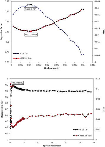
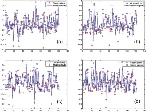
Figure 7. The best and the worst validation results of the selected radial basis networks using the test dataset. Validation of test data for (a) 5-day ahead forecasting with R = 0.9178 and MSE = 0.0172, (b) 10-day ahead forecasting with R = 0.8556 and MSE = 0.0255, (c) 13-day ahead forecasting with R = 0.8636 and MSE = 0.0273, (d) 14-day ahead forecasting with R = 0.9167 and MSE = 0.0158. The vertical axis is the normalized range of water consumption values. Among 14 radial basis networks, models 5 and 14 (which forecast the 5th and 14th day ahead) provide the maximum value of R and minimum value of MSE respectively, models 10 and 13 (which forecast the 10th and 13th day ahead) provide the minimum value of R and maximum value of MSE respectively.
As mentioned in Section 4 (Input variables and data), all selected models that provide the best performance are also evaluated without calendar-based inputs. In all cases, the regression coefficient declines and the MSE measure increases. shows the effect of excluding calendar-based inputs on RBF model performance. Although the model trained without calendar-based inputs follows the general trend of the time series, it can hardly track the daily fluctuations of water consumption. Moreover, including the new inputs results in a significant improvement in capability of all models to forecast large consumption values (values placed above the 80% bound of the historical water consumption range) (). Overall results for all networks and impacts of excluding calendar-based inputs on the results of MLP-BP, CF-BP and RBF models are presented in .
Figure 8. The actual time series vs the forecasts of the selected radial basis network trained with/without calendar-based inputs. Forecasts from 100 runs of the radial basis network are exactly the same.
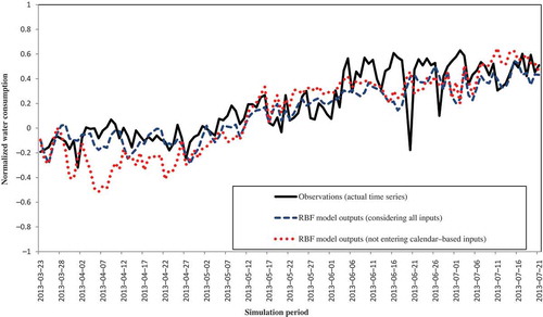
Table 3. Overall results of the three types of neural networks.
All applied ANN models are initialized randomly. The effect of random initialization of ANN weights on model performance has to be studied rigorously through the verification process (Napolitano et al. Citation2011). Thereafter, several hundred repetitions are carried out to estimate the variation range of forecasting values for all models (demonstrated in the Appendix). Evaluating the precise effect of random initialization of weights and comparing the results of experimental repetitions, training and validation datasets are selected likewise for all models (last 10% of the data are selected as the validation/test dataset). All runs also address the adverse impact of excluding calendar-based inputs on the values of performance criteria. Repetitions show that simpler models (which have fewer connections, neurons and layers) result in more stable forecasts. Hence, from the point of view of stability, RBF and MLP-BP models maintain approximately constant forecasting values ( and ). However, CF-BP models seem to be highly susceptible to random initialization of weights. Although a four-hidden-layer CF-BP network with 3-6-1-4 neurons in the hidden layers performs better than a one-hidden-layer network, the simpler model (one-hidden-layer network) provides more stable outputs through repetitions ( and ).
7 Summary and conclusions
In this paper, we proposed some ANN-based models for short-term forecasting of domestic water consumption under peculiar fluctuations in population. Since the model inputs were different for each lead time of water demand forecasting, 14 different networks were developed to predict daily water consumption 1–14 days ahead (a network for each day). The idea of using new calendar-based variables to deal with population fluctuations was evaluated. Validation tests showed that a radial basis function neural network trained by patterns including calendar-based inputs provides the best results in comparison with MLP-BP and CF-BP networks. To investigate the impact of random initialization of the weights and biases of networks and the effect of new inputs on performance measures, several hundred experiments were conducted. It was shown that in 58.89% of the four-hidden-layer CF-BP model runs, 61.14% of the one-hidden-layer CF-BP model runs, 71.07% of the one-hidden-layer MLP-BP model runs and 82.14% of the RBF model runs, the values of performance measures are improved by including the calendar-based inputs. Repetitions likewise indicated poor stability of CF-BP network outputs and qualified the RBF model as the most stable network, having unchanging forecasts for all runs. It seems that the existence of wild fluctuations in population reduces the accuracy and capability of neural networks in water demand forecasting problems. However, this level of precision is still acceptable for short-term water resources planning and management. According to the Appendix, and , the calendar-based inputs can be taken into account to reduce the adverse effects of population fluctuations in tourist cities. This consideration helps networks (especially those that are not highly susceptible to random initialization of connection weights) to provide more accurate water demand forecasting. Significant improvement of the models’ performance was highlighted in forecasting large consumption values. In future work, the results of stochastic modelling of the inputs time series can be compared with the results of the models proposed in this paper. The results of the ANN-based models can also be compared with those of other soft computing techniques.
Acknowledgements
This research was part of a project entitled “Multiobjective optimal operation scheduling for pumping stations of the Doosti water transmission system to the Mashhad city” and was supported by the Doosti Water Transmission System Operation Department of the Khorasan Razavi Regional Water Authority. We hereby acknowledge the great support of Mr Hosein Esmaeliyan and Mr Hamid Mohammadzade.
Disclosure statement
No potential conflict of interest was reported by the author(s).
References
- Aqil, M., et al., 2007. A comparative study of artificial neural networks and neuro-fuzzy in continuous modeling of the daily and hourly behaviour of runoff. Journal of Hydrology, 337 (1–2), 22–34. doi:10.1016/j.jhydrol.2007.01.013
- Billings, R.B. and Agthe, D.E., 1998. State-space versus multiple regression for forecasting urban water demand. Journal of Water Resources Planning and Management, 124 (2), 113–117. doi:10.1061/(ASCE)0733-9496(1998)124:2(113)
- Campisi-Pinto, S., Adamowski, J., and Oron, G., 2012. Forecasting urban water demand via wavelet-denoising and neural network models. Case study: city of syracuse, Italy. Water Resources Management, 26 (12), 3539–3558. doi:10.1007/s11269-012-0089-y
- Donkor, E.A., et al., 2014. Urban water demand forecasting: Review of methods and models. Journal of Water Resources Planning and Management, 140 (2), 146–159. doi:10.1061/(ASCE)WR.1943-5452.0000314
- Fausett, L., 1994. Fundamentals of neural networks: architectures, algorithms, and applications. Upper Saddle River, NJ: Prentice-Hall.
- Felfelani, F., Jalali Movahed, A., and Zarghami, M., 2013. Simulating hedging rules for effective reservoir operation by using system dynamics: a case study of Dez Reservoir, Iran. Lake and Reservoir Management, 29 (2), 126–140. doi:10.1080/10402381.2013.801542
- Filik, U.B. and Kurban, M., 2007. A new approach for the short-term load forecasting with autoregressive and artificial neural network models. International Journal of Computational Intelligence Research, 3 (1), 66–71.
- Firat, M., Turan, M.E., and Yurdusev, M.A., 2009. Comparative analysis of fuzzy inference systems for water consumption time series prediction. Journal of Hydrology, 374 (3–4), 235–241. doi:10.1016/j.jhydrol.2009.06.013
- Firat, M., Turan, M.E., and Yurdusev, M.A., 2010. Comparative analysis of neural network techniques for predicting water consumption time series. Journal of Hydrology, 384 (1–2), 46–51. doi:10.1016/j.jhydrol.2010.01.005
- Ghiassi, M., Zimbra, D.K., and Saidane, H., 2008. Urban water demand forecasting with a dynamic artificial neural network model. Journal of Water Resources Planning and Management, 134 (2), 138–146. doi:10.1061/(ASCE)0733-9496(2008)134:2(138)
- Giustolisi, O. and Simeone, V., 2006. Optimal design of artificial neural networks by a multi-objective strategy: groundwater level predictions. Hydrological Sciences Journal, 51 (3), 502–523. doi:10.1623/hysj.51.3.502
- Hagan, M.T., Demuth, H.B., and Beale, M.H., 1996. Neural network design. Boston, MA: PWS.
- Hedayat, A., et al., 2009. Estimation of research reactor core parameters using cascade feed forward artificial neural networks. Progress in Nuclear Energy, 51 (6–7), 709–718. doi:10.1016/j.pnucene.2009.03.004
- Herrera, M., et al., 2010. Predictive models for forecasting hourly urban water demand. Journal of Hydrology, 387 (1–2), 141–150. doi:10.1016/j.jhydrol.2010.04.005
- Homwongs, C., Sastri, T., and Foster III, J.W., 1994. Adaptive forecasting of hourly municipal water consumption. Journal of Water Resources Planning and Management, 120 (6), 888–905. doi:10.1061/(ASCE)0733-9496(1994)120:6(888)
- Jowitt, P.W. and Xu, C., 1992. Demand forecasting for water distribution systems. Civil Engineering Systems, 9 (2), 105–121. doi:10.1080/02630259208970643
- Lin, J.-Y., Cheng, C.-T., and Chau, K.-W., 2006. Using support vector machines for long-term discharge prediction. Hydrological Sciences Journal, 51 (4), 599–612. doi:10.1623/hysj.51.4.599
- Luk, K., Ball, J., and Sharma, A., 2000. A study of optimal model lag and spatial inputs to artificial neural network for rainfall forecasting. Journal of Hydrology, 227 (1–4), 56–65. doi:10.1016/S0022-1694(99)00165-1
- Napolitano, G., Serinaldi, F., and See, L., 2011. Impact of EMD decomposition and random initialisation of weights in ANN hindcasting of daily stream flow series: an empirical examination. Journal of Hydrology, 406 (3–4), 199–214. doi:10.1016/j.jhydrol.2011.06.015
- Shanker, M., Hu, M.Y., and Hung, M.S., 1996. Effect of data standardization on neural network training. Omega, 24 (4), 385–397. doi:10.1016/0305-0483(96)00010-2
- Tetko, I.V., Livingstone, D.J., and Luik, A.I., 1995. Neural network studies. 1. Comparison of overfitting and overtraining. Journal of Chemical Information and Computer Sciences, 35 (5), 826–833.
- Yurdusev, M.A. and Firat, M., 2009. Adaptive neuro fuzzy inference system approach for municipal water consumption modeling: an application to Izmir, Turkey. Journal of Hydrology, 365 (3–4), 225–234. doi:10.1016/j.jhydrol.2008.11.036
- Zhang, G.P. and Qi, M., 2005. Neural network forecasting for seasonal and trend time series. European Journal of Operational Research, 160 (2), 501–514. doi:10.1016/j.ejor.2003.08.037
- Zhang, J., et al., Short-term water demand forecasting: a case study. ed. 8th annual water distribution systems analysis symposium, 27–30 August 2006 Cincinnati, OH: ASCE Library.
- Zhou, S.L., et al., 2000. Forecasting daily urban water demand: a case study of Melbourne. Journal of Hydrology, 236 (3–4), 153–164. doi:10.1016/S0022-1694(00)00287-0
Appendix
To rigorously study the effect of random initialization of ANN weights on model performance, several hundred repetitions were carried out. The results of these runs were used to estimate the variation range of forecasting values for all ANN models and are illustrated in the following tables and figures.
Figure A1. The actual time series vs the forecast offset resulting from 100 multilayer perceptron model runs. + signs represent forecasts of the model trained with all inputs and the dashed line connects their mean values in each forward lead time. Dots (red) represent forecasts of the model trained excluding calendar-based inputs and the dotted (red) line connects their mean values in each forward lead time.
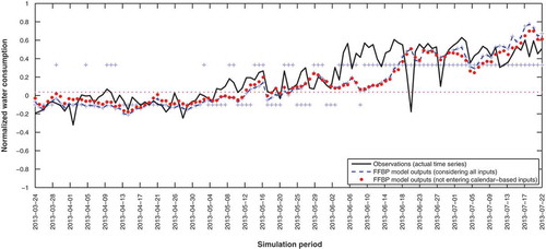
Figure A2. The actual time series vs the forecast offset resulting from 100 one-hidden-layer cascade-forward model runs. Symbols as in Fig. A1.
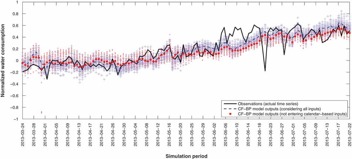
Figure A3. The actual time series vs the forecast offset resulting from 100 four-hidden-layer cascade-forward model runs. Symbols as in Fig. A1.
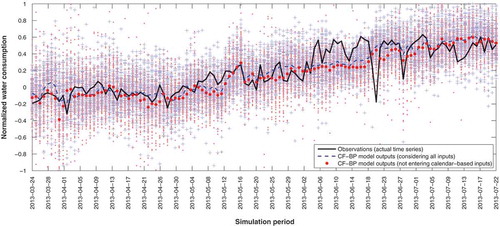
Table A1. Overall results of all repetitions for multilayer perceptron and radial basis function models.
Table A2. Overall results of all repetitions for one-hidden-layer and four-hidden-layer cascade-forward networks.