Predictability in dice motion: how does it differ from hydro-meteorological processes?

ABSTRACT

From ancient times dice have been used to denote randomness. A dice throw experiment is set up in order to examine the predictability of the die orientation through time using visualization techniques. We apply and compare a deterministic-chaotic model and a stochastic model and we show that both suggest predictability in die motion that deteriorates with time, just as in hydro-meteorological processes. Namely, a die’s trajectory can be predictable for short horizons and unpredictable for long ones. Furthermore, we show that the same models can be applied, with satisfactory results, to high temporal resolution time series of rainfall intensity and wind speed magnitude, occurring during mild and strong weather conditions. The difference among the experimental and two natural processes is in the time length of the high-predictability window, which is of the order of 0.1 s, 10 min and 1 h for dice, rainfall and wind processes, respectively.

KEYWORDS:

• stochastic models
• deterministic-chaotic models
• predictability
• uncertainty
• Hurst-Kolmogorov behaviour
• rainfall
• wind

Editor Z.W. Kundzewicz; Associate editor E. Eris

1 Introduction

In principle, one should be able to predict the trajectory and outcome of a die throw by solving the classical deterministic equations of motion; however, the die has been a popular symbol of randomness. This has been the case from ancient times, as revealed in the famous quotation by Heraclitus (c. 540–480 BC; Fragment 52) “Αἰών παῖς ἐστι παίζων πεσσεύων” (“Time is a child playing, throwing dice”). The die’s first appearance in history is uncertain but, as evidenced by archaeological findings, games with cube-shaped dice were widespread in ancient Greece, Egypt and Persia. Dice were also used in temples as a form of divination for oracles and sometimes even restricted or prohibited by law, perhaps for the fear of gamblers’ growing passion to challenge uncertainty (Vasilopoulou 2003).

Despite dice games originating from ancient times, little has been carried out in terms of explicit trajectory determination through deterministic classical mechanics (see Nagler and Richter 2008, Kapitaniak et al. 2012). Recently, Strzalko et al. (2010) studied the Newtonian dynamics of a three-dimensional die throw and noticed a larger probability for the outcome face of the die to be the face looking down at the beginning of the throw, which makes the die not fair by dynamics. However, the probability of the die landing on a face should approach the same value for any face, for large values of the initial rotational and potential energy, and a large number of die bounces. Contrariwise to deterministic analyses, real experiments with dice have not been uncommon. In a letter to Francis Galton (1894), Raphael Weldon, a British statistician and evolutionary biologist, reported the results of 26 306 rolls from 12 different dice; the outcomes showed a statistically significant bias toward fives and sixes, with an observed frequency approximately 0.3377 against the theoretical one of 1/3 (see Labby 2009). Labby (2009) repeated Weldon’s experiment (26 306 rolls from 12 dice) after automating the way the die is released, and reported outcomes close to those expected from a fair die (i.e. 1/6 for each side). This result strengthened the assumption that Weldon’s dice were not fair by construction. Generally, a die throw is considered to be fair as long as it is constructed with six symmetric and homogenous faces (Diaconis and Keller 1989) and for large initial rotational energy (Strzalko et al. 2010). Experiments of the same kind have also been examined in the past in coin tossing (Jaynes 1996, ch. 10; Diaconis et al. 2007). According to Strzalko et al. (2008), a significant factor influencing the coin orientation and final outcome is the coin’s bouncing. Particularly, they observed that successive impacts introduce a small dependence on the initial conditions leading to a transient chaotic behaviour. Similar observations are noticed in the analysis by Kapitaniak et al. (2012) of a die’s trajectory, where lower dependency in the initial conditions was noticed when the die’s bounces are increasing and energy status is decreasing. This observation allowed the speculation that, as knowledge of the initial conditions becomes more accurate, the die orientation with time and the final outcome of a die throw can be more predictable, and thus the experiment tends to be repeatable. Nevertheless, in experiments with no control of the surrounding environment, it is impractical to fully determine and reproduce the initial conditions (e.g. initial orientation of the die, magnitude and direction of the initial or angular momentum). Although in theory one could replicate in an exact way the initial conditions of a die throw, there could be numerous reasons for the die path to change during its course. Since the classical Newtonian laws can lead to chaotic trajectories, this infinitesimal change could completely alter the rest of the die’s trajectory and, consequently, the outcome. For example, the smallest imperfections in the die’s shape or inhomogeneities in its density, external forces that may occur during the throw, such as air viscosity, table friction, elasticity etc., could vaguely diversify the die’s orientation. Nagler and Richter (2008) describe the die’s throw behaviour as pseudorandom since its trajectory is governed by deterministic laws while it is extremely sensitive to initial conditions. However, Koutsoyiannis (2010) argues that it is a false dichotomy to distinguish deterministic from random. Rather, randomness is none other than unpredictability, which can emerge even if the dynamics is fully deterministic (see Appendix B for an example of a chaotic system resulting from the numerical solution of a set of linear differential equations). According to this view, natural process predictability (rooted to deterministic laws) and unpredictability (i.e. randomness) coexist and should not be considered as separate or additive components. A characteristic example of a natural system considered as fully predictable is the Earth’s orbital motion, which greatly affects the Earth’s climate (e.g. Markonis and Koutsoyiannis 2013). Specifically, the Earth’s location can become unpredictable, given a scale of precision, in a finite time window (35 to 50 million years, according to Laskar, 1999). Since a die’s trajectory is governed by deterministic laws, the related uncertainty should emerge as in any other physical process. Hence, there must also exist a time window for which predictability dominates over unpredictability. In other words, a die’s trajectory should be predictable for short horizons and unpredictable for long ones.

In this paper, we reconsider the uncertainty related to dice throwing. We conduct dice throw experiments to estimate a predictability window in a practical manner, without implementing equations based on first principles (all data used in the analysis are available at http://www.itia.ntua.gr/en/docinfo/1538/). Furthermore, we apply the same models to high temporal resolution series of rainfall intensity and wind speed magnitude, which occurred during mild and strong weather conditions, to acquire an insight into their similarities and differences in the uncertainty of the process. The predictability windows are estimated based on two types of model: one stochastic model fitted on experimental data using different time scales, and one deterministic-chaotic model (also known as the analogue model) that utilizes observed patterns assuming some repeatability in the process. For validation reasons, the aforementioned models are also compared to benchmark ones. Certainly, the estimated predictability windows are of practical importance only for the examined type of dice experiments and hydro-meteorological process realizations; nevertheless, this analysis can improve our perception of what predictability and unpredictability (or randomness) are.

2 Data description

In this section, we describe the die throw experimental set-up and analysis techniques, as well as information related to the field observations of small-scale rainfall intensities and wind speed magnitude.

2.1 Experimental set-up of die throw

A simple mechanism is constructed with a box and a high-speed camera in order to record the die’s motion for further analysis (see also Dimitriadis et al. 2013). For this experiment we use a wooden box painted white (to easily distinguish it from the die), with dimensions 30 × 30 × 30 cm. Each side of the die represents one number from 1 to 6, so that the sum of two opposite sides is always 7. The die is of acetate material with smoothed corners, has dimensions 1.5 × 1.5 × 1.5 cm and weighs 4 g. Each side of the die is painted a different colour (Fig. 1): yellow, green, magenta, blue, red and black, for the 1, 2, …, 6 pips, respectively (Table 1). Instead of the primary colour cyan, we use black, as that is easier to trace in contrast to the white colour of the box. The height from which the die is released (with zero initial momentum) or thrown remains constant for all experiments (30 cm). However, the die is released or thrown with a random initial orientation and momentum, so that the results of this study are independent of the initial conditions. Specifically, 123 die throws are performed in total, 52 with initial angular momentum in addition to the initial potential energy and 71 with only the initial potential energy. Despite the similar initial energy status of the die throws, the duration of each throw varied from 1 to 9 s, mostly due to the die’s cubic shape which allowed energy to dissipate at different rates (see Fig. 3).

Figure 1. Mixed combination of frames taken from all the die throw experiments.

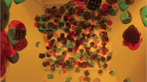
Table 1. (a) Definitions of variables x, y and z that represent proportions of each pair of opposite colours and (b) the eight possible colour/pips triplets, i.e. combinations of three successive colours.

(a) Value →	−1		1
Variable ↓	Colour	Pips	Colour	Pips
x	yellow	1	black	6
y	magenta	3	blue	4
z	red	5	green	2
(b) Colour triplets (by pips)
1^st	2	4	6
2^nd	4	5	6
3^rd	2	3	6
4^th	3	5	6
5^th	1	2	4
6^th	1	4	5
7^th	1	2	3
8^th	1	3	5

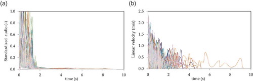
The visualization of the die’s trajectory is done via a digital camera with a pixel density of 0.045 cm/pixel and a frame resolution of 120 Hz. The camera is placed in a standard location and symmetrically to the top of the box. The video is analysed by frames and numerical codes are assigned to coloured pixels based on the HSL system (i.e. hue–saturation–lightness colour representation) and the die’s position inside the box. Specifically, three coordinates are recorded based on the Cartesian orthogonal system; two are taken from the box’s plan view (denoted x_c and y_c) and one corresponding to die’s height (denoted z_c) is estimated from the die’s area (the higher the die, the larger the area; Fig. 2). Moreover, the area of each colour traced by the camera is estimated and then transformed to a dimensionless value divided by the total traced area of the die. In this way, the orientation of the die in each frame can also be estimated through the traced colour triplets, i.e. combinations of three successive colours (Table 1; e.g. Fig. 2(f)). Note that pixels not assigned to any colour (due to relatively low resolution and blurriness of the camera) are approximately 30% of the total traced die area on average. Finally, the audio is transformed to a dimensionless index from 0 to 1 (with 1 indicating the highest sound produced in each experiment) and can be used to record the times the die bounces, colliding with the bottom or sides of the box and contributing in this way to sudden changes in the die’s orientation, to its orbit and, as a result, to the final outcome. We observe in Fig. 3 that the die’s potential energy status (roughly estimated through the noise produced by the die’s bounces) decays faster than its kinetic energy status (roughly estimated through linear velocity). Seemingly, most of the die’s energy dissipation occurs before approximately 1.5 s, regardless of the initial conditions of the die throw (Fig. 3). Based on these observations, we expect predictability to improve after the first 1.5 s.

Figure 2. Selected frames showing the die’s trajectory from experiments number (a) 48 and (b) 78; (c, d) the three Cartesian coordinates (denoted x_c, y_c and z_c for length (left–right), width (down–up) and height, respectively); (e) the colour triplets (corresponding to one of the eight possible combinations of the three neighbouring and most dominant colours; see Table 1 for the definition); and (f) the standardized audio index (representing the sound the die makes when colliding with the box).

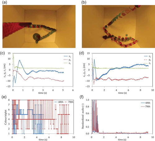
Figure 3. (a) Standardized audios, showing the time the die collides with the box (picks) and (b) linear velocities (calculated from the distance the die covers in two successive frames) for all experiments.

To describe the die orientation we use three variables (x, y and z) representing proportions of each colour, as viewed from above, each of which varies in [−1,1], with x, y, z = 1 corresponding to black, blue or green, respectively, and with x, y, z = −1 corresponding to the colour of the opposite side, that is yellow, magenta or red, respectively (see Table 1 and Fig. 4).

Figure 4. Time series of variables x, y and z for experiments 48 (a, b, c) and 78 (d, e, f); in both experiments the outcome was green.

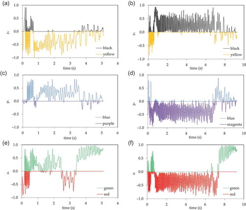
However, these variables are not stochastically independent of each other because of the obvious relationship:

(1)

The following transformation produces a set of independent variables u, v and w, where u and v vary in [−1,1] and w is a two-valued variable taking the value either −1 or 1:

(2)

The inverse transformation is:

(3)

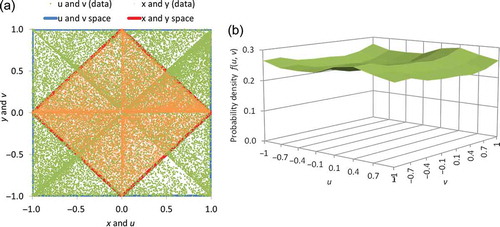
In Fig. 5, the plots of all experimental points and of the probability density function (pdf) show that u and v are independent and fairly uniformly distributed, with the exception of the more probable states where u ± v = 0 (corresponding to one of the final outcomes). Note that w outcomes are also nearly uniform with marginal probabilities and .

Figure 5. Plot of (a) all (x,y) and (u,v) points from all experiments and (b) the probability density function of (u,v).

2.2 Hydro-meteorological time series

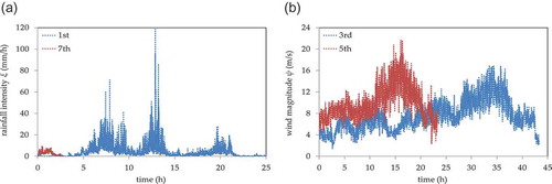
We choose a set of high-resolution time series of rainfall intensities (denoted ξ and measured in mm/h) and wind speed (denoted ψ and measured in m/s). The rainfall intensities dataset consists of seven time series (Fig. 6(a)), with a 10 s time step, recorded during various weather states (high and low rainfall rates) by the Hydrometeorology Laboratory at the University of Iowa (for more information concerning the database see Georgakakos et al. 1994). The wind speed database consists of five time series (Fig. 5(b)), with a 1 min time step, recorded during various weather states (such as strong breeze and storm events) by a sonic anemometer on a meteorological tower located at Beaumont, Kansas, and provided by NCAR/EOL (http://data.eol.ucar.edu/). We have chosen these processes as they are of great interest in hydro-meteorology and are often regarded as random-driven processes.

Figure 6. (a) Rainfall events 1 and 7 (provided by the Hydrometeorology Laboratory at the University of Iowa) and (b) wind events 3 and 5 (provided by NCAR/EOL).

3 Prediction models

In this section, we use several prediction models in order to illustrate the differences and similarities in predictability of a die’s motion (in particular, its orientation) and of two hydro-meteorological processes (rainfall intensity and wind speed magnitude). Specifically, we apply two types of prediction models in each process and compare their outputs, for the same process and between the other processes, in terms of the Nash and Sutcliffe (1970) efficiency coefficient defined as:

(4)

where d is an index for the sequential number of the die experiments, rainfall or wind events; i denotes time; n is the total number of experiments, or of recorded rainfall or wind events (n = 123 for the die throw experiment, n = 7 for the rainfall and n = 5 for the wind events); b_d is the total number of recorded frames in the dth experiment, rainfall or wind event; s represents the variable of interest (u, v and w, ξ or ψ); is the vector , transformed from the originally observed , for the die throw, the one-dimensional rainfall intensity, , for the rainfall events and the one-dimensional wind speed magnitude, , for the wind events; is the mean vector for the process; and is the discrete-time vector estimated from the model.

The prediction models described below are checked against two naïve benchmark models. For the first benchmark model (abbreviated B1), the prediction is considered to be the average state (hence, F = 0), i.e.:

(5)

where tΔ is the present time in s (t denotes dimensionless time), lΔ the lead time of prediction in s (l > 0), Δ the sampling frequency (equal to 1/120 s for the die throw game, 10 s for the rainfall events and 1 min for the wind events) and the process mean (i.e. , mm/h and m/s).

Although the mean state is not permissible per se, the B1 can be used as a threshold, since any model worse than this (i.e. F < 0), is totally useless. At the second benchmark model (abbreviated B2), the prediction is considered to be the current state regardless of how long the lead time lΔ is, i.e.:

(6)

Regarding the more sophisticated models applied, a parsimonious linear stochastic model is first tested (described in detail in Appendix A), which predicts the state at lead time lΔ, based on a number of weighted present and past states , where , as:

(7)

where c_q are weighting factors and p is the total number of past states.

The coefficients c_q are determined on the basis of a generalized Hurst-Kolmogorov stochastic process, which incorporates both short- and long-term persistence using very few model parameters. Once these parameters are estimated from the data, in terms of their climacograms (i.e. variance of the time-averaged process over averaging time scale; Koutsoyiannis 2010, 2015), the coefficients c_q can be analytically derived as detailed in Appendix A.

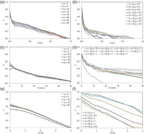
Applying a sensitivity analysis to this model (Appendix A; Fig. A2), we deduce that for the die process a value of p = 20 (which corresponds to time length ~0.17 s) works relatively well (on the concept that it is a small value producing a large F), for lead time, lΔ, varying from 8 ms to 1.5 s (for larger values of p we have a negligible improvement of the efficiency). Similarly, for the rainfall process, we come to the conclusion that p = 15 (corresponding to 150 s) is adequate, for lΔ varying from 10 s to 1 h. Finally, for the wind process, the model’s performance is sufficient for p = 5 (corresponding to 5 min), for lΔ varying from 1 min to 6 h.

Additionally, we apply a deterministic data-driven model (also known as the analogue model, e.g. Koutsoyiannis et al. 2008), which is often used in chaotic systems (such as the classical Lorenz set of differential equations shown in Appendix B). This model is purely data-driven, since it does not use any mathematical expressions between variables. Notably, to predict a state based on h past states , for r varying from 1 to h, we explore the database of all experiments or events to detect k similar states (called neighbours or analogues), , so that for each j (varying from 1 to k) the expression below holds for all r:

(8)

where g is an error threshold.

Subsequently, we obtain for each neighbour the state at time , i.e. , and predict the state at lead time lΔ as:

(9)

Applying again a sensitivity analysis to this model (Appendix A; Fig. A2), we estimate that a number of past values h = 15 (which corresponds to time length ~0.125 s) and a threshold g = 0.5 performs relatively well for the die process. Similarly, for the rainfall process, we infer that the model performance is adequate for h = 15 (which corresponds to time length 150 s) and a threshold g = 2 mm/h. Finally, we conclude that h = 5 (which corresponds to time length 5 min) and a threshold g = 0.5 m/s work sufficiently for the wind process.

Note that for the estimation of the above model parameters we adopt two extra criteria. The first is that both models’ efficiency coefficients should be larger than that of the B2 model (at least for most of the lead times). The second is that their efficiency values should be estimated from a reasonably large set of tracked neighbours (>10% of the total number of realizations for each process). Due to high variances of the time-averaged process (or, equivalently, high autocorrelations), shown in Fig. A1 of Appendix A, it is expected that the B2 model will perform sufficiently well for fairly small lead times. This can be verified in Fig. 7, which depicts the results for the four prediction models, for die experiment 48, the first rainfall event and the third wind event.

Figure 7. Comparisons between B1, B2, stochastic and analogue models for the die experiment (a and b), the observed rainfall intensities (c and d) and the observed wind speed (e and f). The left column (a, c and e) represents the application of the models to all experiments and events and the right column (b, d and f) to individual ones.

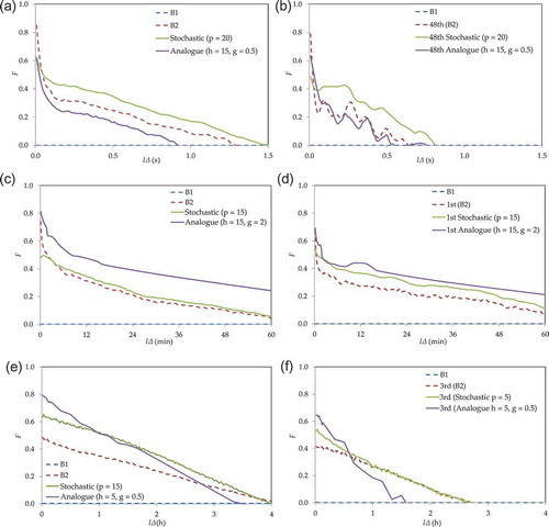
The stochastic model provides relatively good predictions (F ≳ 0.5 and efficiency coefficients larger than the B1 and B2 models) for lead times lΔ ≲ 0.1 s for the die experiments (with a range approximately from 0.05 to 0.5 s), ≲10 min for the rainfall events (with a range approximately from 1 to 30 min) and ≲1 h for the wind events (with a range approximately from 0.1 to 2 h). The analogue model produces smaller F values than the B2 model for the die and the wind processes, and larger values in the case of the rainfall process (but smaller than the stochastic model). Predictability is generally good for short lead times; however, the situation deteriorates for longer ones. Finally, we define and estimate the predictability window (that is the window beyond which the process is considered as unpredictable), as the time window beyond which the efficiency coefficient F becomes negative. Specifically, predictability is superior to the case of a pure random process (B1) for lead times lΔ ≲ 1.5 s for the die throw, ≲2 h for the rainfall and ≲4 h for the wind process.

4 Summary and conclusions

A die throw experiment is performed with varying initial conditions (in terms of rotational energy and die orientation) in order to investigate the predictability time window of the die’s trajectory. We apply two types of models, one solely data-driven model (of deterministic-chaotic type) which exploits observed patterns similar to the present one to predict future states. Also, a stochastic model is applied for the first time (to the authors’ knowledge) in this type of experiment. For this model, the climacogram (variance of the time-averaged process over averaging time scale) is estimated and fitted to a generalized Hurst-Kolmogorov process. Subsequently, the best linear unbiased estimator (BLUE) method is applied to determine weighting factors for the prediction model components. The predictability time window is estimated such as the Nash-Sutcliffe efficiency coefficient is greater than 0.5 and greater than those estimated from simple benchmark models. Furthermore, the same prediction models are applied to rainfall intensity and wind speed magnitude processes.

The results show that a die’s trajectory is fairly predictable for time windows of approximately 0.1 s, and this time window becomes 10 min for rainfall intensity and 1 h for wind speed. Thus, dice seem to behave like any other common physical system: predictable for short horizons, unpredictable for long horizons. The main difference between dice trajectories and other common physical systems is that they enable unpredictability very quickly. This important result, though holding only for the examined type of die experiment and hydro-meteorological processes, highlights the fact that the die trajectory should not be considered as completely unpredictable. Thus, it helps to develop a unified perception for all natural phenomena and expel dichotomies such as random vs deterministic; there is no such thing as a ‘virus of randomness’ infecting some phenomena to make them random, leaving other phenomena uninfected. It seems rather that both randomness and predictability coexist and are intrinsic to natural systems, which can be deterministic and random at the same time, depending on the prediction horizon and the time scale. On this basis, the uncertainty in a geophysical process can be both aleatory (‘alea’ being Latin for ‘dice’) and epistemic (as in principle we could know perfectly the initial conditions and the equations of motion but in practice we do not). Therefore, dichotomies such as ‘deterministic vs random’ and ‘aleatory vs epistemic’ may be false ones and may lead to paradoxes.

Finally, we observe that the largest Hurst coefficient (estimated from the stochastic processes) corresponds to the wind process (H ≈ 0.95), the intermediate to the rainfall process (H ≈ 0.9), and the smallest one to the die process (0.5 < H < 0.6). It is interesting to observe that as H increases so does the predictability time window. This may seem a paradox, since high H is related to high uncertainty. The latter statement is indeed true but only for long time scales. As thoroughly analysed in Koutsoyiannis (2011), processes with high H exhibit smaller uncertainty (i.e. smaller entropy production) for short time periods, in comparison with processes with smaller H. Conversely, if averages at large time scales are considered, then dice become more predictable as they will soon develop a time average of 3.5; this is also strengthened by the fact that a die is orientation limited to a combination of six faces, while rainfall and wind processes have infinite possible patterns and thus can be more unpredictable for long horizons and long time scales.

Acknowledgements

Wind time series used in the analysis are made available on-line by NCAR/EOL under the sponsorship of the National Science Foundation (http://data.eol.ucar.edu/). The seven storm events were recorded by the Hydrometeorology Laboratory at the University of Iowa. We thank the editors Zbigniew Kundzewicz and Ebru Eris, the reviewer and the eponymous reviewer Francesco Laio for the constructive comments which helped us improve the paper.

Disclosure statement

No potential conflict of interest was reported by the authors.

Additional information

Funding

This work was partly funded by the Greek General Secretariat for Research and Technology through the research project Combined REnewable Systems for Sustainable Energy DevelOpment (CRESSENDO, grant number 5145).

Appendix A

In this appendix, we describe the stochastic prediction model (used in Section 3). Additionally, we show the results from the sensitivity analysis of the stochastic model as well as the analogue model (described in Section 3).

The linear stochastic model predicts the state at lead time lΔ, i.e. , based on the linear aggregation of weighted past states, i.e. , with c_q the weighting factors (equation (7); see Section 3 for notation). Before we estimate the weights, it is necessary to presume a model of the stochastic structure for each process. The observed climacogram (i.e. variance of the time-averaged process over averaging time scale) in Fig. A1, shows the strong dependence of the die orientation, rainfall intensity and wind speed on time (long-term, rather than short-term persistence). This enables stochastic predictability up to a certain lead time. Regarding the fitting method of the stochastic model, we choose the climacogram (Koutsoyiannis 2010, 2015) and for the model type we choose the generalized Hurst-Kolmogorov (gHK) process. The climacogram is chosen because it results in smaller estimation errors in comparison to autocovariance (or autocorrelation) and a power spectrum for this type of models (a thorough analysis of this has been made elsewhere; Dimitriadis and Koutsoyiannis 2015). Also, the gHK model is chosen as it can exhibit both Markovian (short-term) and HK (long-term) persistence, depending on the value of the Hurst coefficient (defined as H = 1 − b/2, where b is the true log-log slope of the climacogram at large scales). In particular, the Markovian case appears when H = 0.5, while for greater values it signifies long-term persistence. By definition, the true autocovariance, c(τ) for lag τ, of a gHK process is (Koutsoyiannis 2013, Dimitriadis and Koutsoyiannis 2015):

(A1)

Figure A1. True, expected and averaged empirical climacograms for (a) u and , (b) , (c) and (d) ψ.

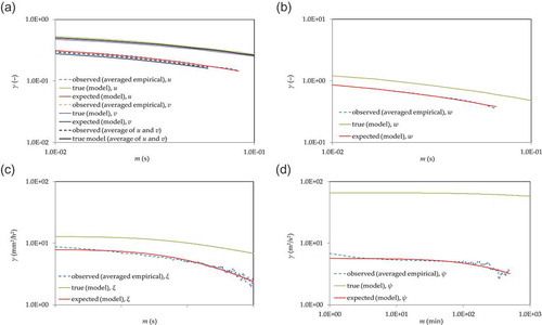
where λ is the variance at an instantaneous time scale and q and b are the scale and long-term persistence parameters, respectively. Its climacogram, γ(m), for time scale m ≔ kΔ (with k the dimensionless discrete-time scale), is:

(A2)

while the classical estimator of the true climacogram is biased (due to finite sample size) and is given by:

(A3)

where Δ is the time resolution parameter (1/120 s for the die experiments, 10 s for the rainfall events and 1 min for the wind events) and N is the sample size.

For consideration of the bias effect due to varying sample sizes n of the die experiments and rainfall and wind events, we estimated the average of all empirical climacograms for experiments and events of similar sample size. However, due to the strong climacogram structure of all three processes, the varying sample size has a small effect on the shape of the climacogram for scales up to approximately 10% of the sample size (following the rule of thumb for this type of model, as analysed in Dimitriadis and Koutsoyiannis 2015) and thus we consider the averaged empirical climacogram to represent the expected one.

The fitted models are shown in Fig. A1 in terms of their climacograms (a stochastic analysis based on the autocorrelation of the examined rainfall events can be seen in Papalexiou et al. 2011). Their parameters are: for the u and v symmetric variables of the die process λ = 0.6, q = 0.013 s and b = 0.83 (H ≈ 0.6); for the w variable λ = 1.635, q = 0.0082 s and b ≈ 1.0 (H ≈ 0.5); for the rainfall process λ = 12.874 mm²/h², q = 130 s and b = 0.22 (H ≈ 0.9); and for the wind process λ = 65.84 m²/s², q = 86 min and b = 0.09 (H ≈ 0.95). We observe that the scale parameter q and Hurst coefficient H are largest in the wind process and smallest in the die process.

Finally, we apply the best linear unbiased estimator (BLUE) method (Koutsoyiannis and Langousis 2011), under the assumption of stationarity and isotropy, to estimate the weighting factors c_q (so as the sum of them equals unity):

(A4)

where represents the vector of the weighting factors c_q (for q = 0, …, p) and ζ a coefficient related to the Lagrange multiplier of the method; , for all i,j = q, is the positive definite symmetric matrix whose elements are the true (included bias) autocovariances of x, which represents the variable of interest (u, v, w, ξ or ψ) and now is assumed random (denoted by the underscore) for the application of this method; for all q; l is the index for the lead time (l > 0); and the superscript T denotes the transpose of a matrix.

In Fig. A2, we show the sensitivity analysis applied to both stochastic and analogue models, and for each process. Specifically, we apply a variety of p values (i.e. number of present and past states that the model assumes the future state is depending on) for the stochastic model and combinations of h (same as p) and (i.e. error threshold value for secting neighbours) values for the analogue one.

Figure A2. Sensitivity analyses of the stochastic (left column) and analogue (right column) model parameters for the die experiment (a and b), the rainfall intensities (c and d) and the wind speed (e and f).

Appendix B

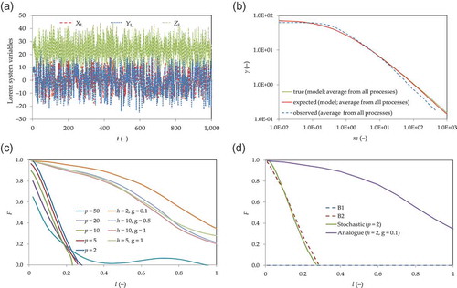
In this appendix, we apply all models described in Section 3 to a set of time series produced by numerically solving Lorenz’s chaotic system (see below). Particularly, applying the Runge-Kutta integration approach (Press et al. 2007), we produce n = 100 time series of the Lorenz-system dimensionless variables (denoted X_L, Y_L and Z_L), with randomly varying initial values of variables between −1 and 1, a time step of d_t = Δ = 0.01 (dimensionless), a total time length of T_L = 10³ (so, each time series contains Ν = 10⁵ data) and with the classical Lorenz-system dimensionless parameters of σ_L = 10, r_L = 8 and b_L = 8/3 (Lorenz 1963):

(B1)

The fifth time series is shown in Fig. B1, along with the results from the stochastic and analogue models. The estimated parameters for the best fitted (Markov-type) stochastic model are λ ≈ 72.8, q ≈ 0.13 for the X_L process, λ ≈ 93.1, q ≈ 0.0836 for Y_L and λ ≈ 272, q ≈ 0.0007 for Z_L, with b ≈ 1.0 (H ≈ 0.5) for all processes (with and ). From the analysis, we conclude that the analogue model with h = 2 (which corresponds to time length 0.02 s) and a threshold of g = 0.1 performs very well as opposed to the stochastic model. The latter’s efficiency factor is slightly higher than that corresponding to the B2 model, only for small lead times and lower than the rest, in contrast with the experimental and natural processes in Fig. 7. We believe this is because the system’s dynamics are relatively simple and no other factors affect the trajectory. Such conditions are never the case in a natural process and thus the performance of the analogue model is usually of the same order (given there are many data available, whereas the stochastic model can be set up with much fewer data). Finally, predictability seems to be generally superior to a pure random process (B1), for lead times lΔ ≲ 1.

Figure B1. (a) Values of X_L, Y_L and Z_L, plotted at a time interval of 0.1, for the fifth time series produced by integrating the classical Lorenz chaotic system. (b) Observed climacogram as well as its true and expected values for the fitted stochastic gHK model (average of X_L, Y_L and Z_L processes). (c) Sensitivity analysis of the analogue and stochastic models and (d) comparison of the optimum stochastic and analogue models with B1 and B2.

References

- Diaconis, P., Holmes, S., and Montgomery, R., 2007. Dynamical Bias in the Coin Toss. SIAM Review, 49 (2), 211–235. doi:10.1137/S0036144504446436
- Diaconis, P. and Keller, J.B., 1989. Fair Dice. American Mathematical Monthly, 96 (4), 337–339.
- Dimitriadis, P. and Koutsoyiannis, D., 2015. Climacogram vs. autocovariance and power spectrum in stochastic modelling for Markovian and Hurst-Kolmogorov processes. Stochastic Environmental Research & Risk Assessment, 29 (6), 1649–1669. doi:10.1007/s00477-015-1023-7
- Dimitriadis, P., Tzouka, K., and Koutsoyiannis, D., 2013. Windows of predictability in dice motion. In: Facets of Uncertainty: 5th EGU Leonardo Conference – Hydrofractals 2013 – STAHY 2013[online], 17–19 October. Kos Island: European Geosciences Union, International Association of Hydrological Sciences, International Union of Geodesy and Geophysics, p. 18. Available from: www.itia.ntua.gr/en/docinfo/1394/ [Accessed 15 Aug 2014] .
- Georgakakos, K.P., et al., 1994. Observation and analysis of Midwestern rain rates. Journal of Applied Meteorology, 33, 1433–1444. doi:10.1175/1520-0450(1994)033<1433:OAAOMR>2.0.CO;2
- Jaynes, E. T., 1996. Probability theory: the logic of science. Cambridge: Cambridge University Press.
- Kapitaniak, M., et al., 2012. The three-dimensional dynamics of dice throw. Chaos, 22 (4), 047504.
- Koutsoyiannis, D., 2010. HESS opinions “A random walk on water”. Hydrology and Earth System Sciences, 14, 585–601. doi:10.5194/hess-14-585-2010
- Koutsoyiannis, D., 2011. Hurst-Kolmogorov dynamics as a result of extremal entropy production. Physica A: Statistical Mechanics and its Applications, 390 (8), 1424–1432. doi:10.1016/j.physa.2010.12.035
- Koutsoyiannis, D., 2013. Encolpion of stochastics: Fundamentals of stochastic processes [online]. Department of Water Resources and Environmental Engineering, National Technical University of Athens, Athens. Available from: http://www.itia.ntua.gr/en/docinfo/1317/ [Accessed 15 Aug 2014].
- Koutsoyiannis, D., 2015. Generic and parsimonious stochastic modelling for hydrology and beyond. Hydrological Sciences Journal. doi:10.1080/02626667.2015.1016950.
- Koutsoyiannis, D. and Langousis, A., 2011. Precipitation. In: P. Wilderer and S. Uhlenbrook, eds. Treatise on water science. Vol. 2: The science of hydrology. Oxford: Academic Press, 27–77.
- Koutsoyiannis, D., Yao, H., and Georgakakos, A., 2008. Medium-range flow prediction for the Nile: a comparison of stochastic and deterministic methods. Hydrological Sciences Journal, 53 (1), 142–164. doi:10.1623/hysj.53.1.142
- Labby, Z., 2009. Weldon’s dice automated. Chance, 22 (4), 6–13. doi:10.1007/s00144-009-0036-8
- Laskar, J., 1999. The limits of Earth orbital calculations for geological time-scale use. Philosophical Transactions of the Royal Society of London A, 357, 1735–1759. doi:10.1098/rsta.1999.0399
- Lorenz, E.N., 1963. Deterministic nonperiodic flow. Journal of the Atmospheric Sciences, 20 (2), 130–141. doi:10.1175/1520-0469(1963)020<0130:DNF>2.0.CO;2
- Markonis, Y. and Koutsoyiannis, D., 2013. Climatic variability over time scales spanning nine orders of magnitude: connecting Milankovitch cycles with Hurst–Kolmogorov dynamics. Surveys in Geophysics, 34 (2), 181–207. doi:10.1007/s10712-012-9208-9
- Nagler, J. and Richter, P., 2008. How random is dice tossing. Physics Review E, 78, 036207. doi:10.1103/PhysRevE.78.036207
- Nash, J.E. and Sutcliffe, J.V., 1970. River flow forecasting through conceptual models part I — a discussion of principles. Journal of Hydrology, 10 (3), 282–290. doi:10.1016/0022-1694(70)90255-6
- Papalexiou, S.M., Koutsoyiannis, D., and Montanari, A., 2011. Can a simple stochastic model generate rich patterns of rainfall events? Journal of Hydrology, 411 (3–4), 279–289. doi:10.1016/j.jhydrol.2011.10.008
- Press, W.H., et al., 2007. Preface to the third edition, numerical recipes: the art of scientific computing. 3rd ed. New York: Cambridge University Press.
- Strzalko, J., et al., 2010. Can the dice be fair by dynamics?. International Journal of Bifurcation and Chaos, 20 (4), 1175–1184. doi:10.1142/S021812741002637X
- Strzalko, J., et al., 2008. Dynamics of coin tossing is predictable. Physics Reports, 469, 59–92. doi:10.1016/j.physrep.2008.08.003
- Vasilopoulou, E., 2003. The child and games in ancient Greek art. Graduating thesis. Aristotle University of Thessaloniki (in Greek).