Improvement and comparison of the rainfall–runoff methods in SWAT at the monsoonal watershed of Baocun, Eastern China

ABSTRACT

A new physics-based rainfall–runoff method of the Soil and Water Assessment Tool (SWAT) was developed, which integrates a water balance (WB) approach with the variable source area (WB-VSA). This approach was further compared with four methods—soil-water-dependent curve number (CN-Soil), evaporation-dependent curve number (CN-ET), Green and Ampt equation (G&A) and WB—in a monsoonal watershed, Eastern China. The regional sensitivity analysis shows that volumetric efficiency coefficient (VE) with river discharges is sensitive to the most parameters of all approaches. The results of model calibration against VE demonstrate that WB-VSA is the most accurate owing to its reflection of the spatial variation of runoff generation as affected by topography and soil properties. Other methods can also mimic baseflow well, but the G&A and CN-ET simulate floods much worse than the saturation excess runoff approaches (WB-VSA, WB and CN-Soil). Meanwhile, CN-Soil as an empirical method fails to simulate groundwater levels. By contrast, WB-VSA captures them best.

Editor M.C. Acreman; Associate editor S. Kanae

KEYWORDS:

• Soil and Water Assessment Tool (SWAT)
• infiltration excess (Horton) runoff
• saturation excess (Dunne) runoff
• water balance
• topographic index
• variable source area

1 Introduction

The Soil and Water Assessment Tool (SWAT) developed by the USDA Agricultural Research Service (ARS) is computationally efficient and capable of continuous simulation of hydrology- and water-related processes over long time periods, which has been proved to be an effective tool for assessing water resource problems over a wide range of scales and environmental conditions (Gassman et al. 2007). The SWAT model provides two methods to estimate overland runoff (i.e. a flow that occurs along a sloping surface). The first option is the Soil Conservation Service curve number procedure (CN) that includes the soil water content dependence (CN-Soil) and the plant evapotranspiration dependence (CN-ET) retention parameter methods (Neitsch et al. 2005). The second option is the Green and Ampt infiltration equation (G&A) (Neitsch et al. 2005).

The CN method is widely used to calculate watershed runoff from rainfall, and is included in many other hydrological softwares, such as HEC-HMS, CREAMS, SWRRB, and EPIC, possibly because of its simplicity, predictability and stability (SCS 1972, Ponce and Hawkins 1996, Grimaldi et al. 2013). It assumes that the ratio of actual retention to potential retention equals the ratio of actual runoff to potential runoff, which was derived from small experimental watersheds with a unique hydrologic soil group and land use (Yuan et al. 2001, Yu 2012). The curve number is a function of the soil type, land use and antecedent moisture condition, so the CN model can be used to estimate the amounts of runoff under varying land use and soil types (Rallison and Miller 1982). However, the CN model has been found to have structural limitations. For example, the CN is based only on total rainfall volume, while rainfall intensity and duration are not considered (King et al. 1999, Jeong et al. 2010). As a result, the method fails to represent runoff rates, pathways and source areas (Tedela et al. 2012). The original purpose of the CN model is to compute streamflow volume (minus baseflow) for a storm, so treating the curve number runoff (that may include some interflow) as only overland flow by SWAT would result in an overestimation of the overland flow (Garen and Moore 2005, Arnold et al. 2011). The unavailability of detailed and descriptive information on soil properties often limits the implementation of complete infiltration schemes (Gabellani et al. 2008). To overcome these limitations, many efforts have been made by modifying the CN schematization (e.g. Yu 1998, Mishra and Singh 2003, Gabellani et al. 2008).

The Green and Ampt (G&A) method was developed to predict infiltration when the excess water was on the surface at all times (Neitsch et al. 2005). Different from the CN method, the G&A is a physically-based method. It assumes that the soil profile is homogeneous, antecedent moisture is uniformly distributed in the soil profile, and the pattern of soil water movement is the saturated plug/piston flow. The physics-based Horton-like methods present parameters that, though measurable to a point, make it difficult to achieve a reliable estimate at the catchment scale. To overcome this limitation, Gabellani et al. (2008) developed an approach that maps the CN values onto the initial infiltration rate of a modified Horton’s equation, which obviously outperforms the CN method on long, multi-peak events. The G&A method requires sub-daily inputs (King et al. 1999, Jeong et al. 2010). As a result, if quality input data are not available, watershed models with the G&A method may not be appropriate (Migliaccio and Srivastava 2007, Jeong et al. 2010).

Both the CN and the G&A approaches are based on the principle of the infiltration excess (Horton overland flow; Walter and Shaw 2005). Horton overland flow occurs when the rainfall rate exceeds the infiltration capacity of the surface soil (Loague et al. 2010). Comparison of the CN and the G&A approaches, based on uncalibrated SWAT simulations, indicated that no significant advantage was obtained by using one approach rather than the other (King et al. 1999, Ficklin and Zhang 2013). However, Kannan et al. (2007) pointed out that the calibrated streamflow results were more accurate using the CN approach when compared to the G&A approach for a small watershed because the G&A approach holds more water in the soil profile and predicts a lower peak runoff rate. Han et al. (2012) found that both the CN and the G&A methods in the SWAT have some limitations in reflecting that soil moisture updates into the surface runoff generation.

Another type of surface runoff process is Dunne overland flow (saturation excess). Dunne overland flow occurs when the rainfall rate is less than the infiltration capacity of the surface soil with small soil-saturation deficit (Dunne 1978, Loague et al. 2010). For Dunne overland flow, surface runoff is contributed by only a portion of a watershed. This concept is often referred to as variable source areas (VSAs). Although the CN approach is derived from the principle of Horton overland flow, Steenhuis et al. (1995) revealed that the CN approach can be revisited for variable source runoff areas. In order to further improve the physical basis of the CN and identify the location of the contributing runoff areas, numerous authors proposed many new models (e.g. SWAT-VSA) by incorporating the soil-topographic index into CN-based watershed models (Lyon et al. 2004, Schneiderman et al. 2007, Easton et al. 2008). However, White et al. (2011) found that the CN-based SWAT-VSA cannot account for the extreme antecedent moisture conditions that are found in monsoonal climates. They incorporated the water balance model (WB) with the spatial adjustments by using a soil wetness index to replace the CN approach, and developed a physics-based SWAT model termed SWAT-WB. They found that SWAT-WB was useful when the rainfall intensity is generally less than the soil infiltration capacity. In SWAT-WB, the effective depth of soil profile is a very important parameter, which is used to reflect the effect of topography on soil saturation deficit. However, SWAT-WB needs to determine the parameter of effective soil depth in each soil wetness class, which brings many inter-correlated parameters and results in difficulties in model calibration.

The primary goal of this study is to improve the SWAT-WB model by establishing an estimation method for the effective depth of soil profile in the water balance model (WB). The improved approach, termed WB-VSA, is further compared with four rainfall–runoff approaches (CN-Soil, CN-ET, G&A and WB) of SWAT in a monsoonal watershed. To assess the model performance and reliability, we firstly used the Regional Sensitivity Analysis method with Latin Hypercube Sampling (LHS-RSA) to analyse the sensitivity of model parameters, and then adopted the automatic optimization method of the Differential Evolution Adaptive Metropolis (DREAM) scheme to calibrate the five models. Lastly, the groundwater levels and the last 2 years of river discharges were employed in validation of the five models.

2 Study area

The Baocun watershed is located in the eastern Jiaodong Peninsula, a part of Shandong Province in China (Fig. 1). The elevation of the watershed ranges from 20 m at the watershed outlet to 220 m above mean sea level at the head-watershed (northern mountain area). The watershed area amounts to 86.7 km². The length of watershed is 16.1 km, the average width is 5.38 km and the average slope is 8.2‰. The climate belongs to the warm temperate zone in a humid monsoon region with an average annual precipitation of 806 mm. There is a considerable inter-annual variation of precipitation. Over the past 50 years, the maximum was observed in 2003 with an annual precipitation of 1220 mm, and the minimum occurred in 1999 when only 384 mm was recorded. Meanwhile, nearly 70% of the annual precipitation occurs in the rainy season from June to September. The average annual potential evaporation is 899 mm (measured by pan evaporation equipment). The average monthly temperature ranges from −0.8°C in January to 24.4°C in August, and the warm months correspond with the moist months.

Figure 1. Location and topography of (a) the Jiaodong peninsula and (b) the Baocun watershed, as well as position of the gauging stations. Database: 1:10 000-scale topographic map.

According to the study of Wang et al. (2002), the Baocun watershed is located in the eastern part of the Jiao-Liao uplift-fault block, and the exposed rocks are mainly of the metamorphic and igneous types. The area was always uplifting and suffering from erosion from the Early Proterozoic era to the Neogene period. Sediments and weathered residuals were deposited in this area until the Cenozoic-Quaternary-Pleistocene. Therefore, the soils are generally shallow. The main land use is cropland, and the dominant crops are peanut, corn and winter wheat. The croplands are farmed three times every 2 years, which is termed crop rotation. The detailed schedule of planting crops is peanut in May, winter wheat in October, and corn in June of the next year.

3 Material and methods

3.1 SWAT model

SWAT is a distributed hydrological model. It describes the spatial distribution of hydrological processes by dividing a watershed into multiple sub-basins, and then further subdividing the sub-basin into multiple hydrologic response units (HRUs) consisting of homogeneous land use, soil characteristics and slope. The HRU is the smallest element of SWAT. The HRU represents percentages of the sub-basin area rather than spatially identified locations. HRUs are independent of each other, mainly including four water storages (surface water, soil water, shallow groundwater and deep aquifer) and five pathways for water movement (surface runoff, evapotranspiration, lateral flow, baseflow, and percolation from soil layer to groundwater aquifer). The model structure of one HRU in the SWAT model is shown in Fig. 2, where ‘Shallow GW’ means the shallow groundwater aquifer, and the arrow is the direction of water movement.

Figure 2. Schematic of main pathways for water movement in SWAT.

3.1.1 Description of the surface runoff generation approaches

3.1.1.1 Curve number approach (CN)

On the basis of the hypothesis that the ratio between potential runoff volume and runoff volume equals the ratio between potential maximum retention and infiltration volume by the SCS curve number approach, a simplified mass balance equation can be obtained (Neitsch et al. 2005):

(1)

where Q_surf is the accumulated overland flow (mm/d), R is the daily rainfall (mm/d), S is the retention parameter (mm) and I_a is the initial abstraction that is commonly approximated as 0.2S. The retention parameter is defined as:

(2)

where CN is the curve number for the day (Table 1), which is a function of the soil type, land cover and antecedent moisture condition.

Table 1. Description of model parameters and their ranges.

Categories	Parameter^a	Range^b		Definition
		LB	UB
Evapotranspiration	v__ESCO	0.01	1	Soil evaporation compensation factor
	v__EPCO	0.01	1	Plant uptake compensation factor
Surface water	r__CN2^c	−0.9	1	Initial curve number for moisture condition II (only in the CN-soil, CN-ET and G&A approaches)
	v__CNCOEF	0.1	10	Plant ET curve number coefficient (only in the CN-ET approach)
	v__EDC^d	0	1	Effective depth of the soil profile (only in the WB and WB-VSA approaches)
	v__OV_N	0.005	0.5	Roughness coefficient of sloping surface
	v__SURLAG	0	24	Surface runoff lag coefficient
Soil water	r__SOL_Z	−0.9	2	Soil thickness (mm)
	r__SOL_BD	−0.6	1	Moist bulk density (g cm^−3)
	r__SOL_AWC	−0.99	3	Available water capacity of the soil layer
	r__SOL_K	−0.99	10	Saturated hydraulic conductivity (mm/d)
Groundwater	v__GW_DELAY	0	60	Groundwater delay time (d)
	v__ALPHA_BF	0	1	Baseflow recession constant
	v__GWQMN	0	1000	Threshold depth of water in the shallow aquifer required for return flow to occur (mm)
	v__RCHRG_DP	0	1	Deep aquifer percolation fraction
	v__REVAPMN	0	1000	Threshold depth of water in the shallow aquifer for revaporization (mm)
	v__GW_REVAP	0.02	0.2	Groundwater revaporization coefficient
Tributary/main channel	v__CH_N1	0.005	0.15	Roughness coefficient of tributary channels
	v__CH_N2	0.005	0.15	Roughness coefficient of main channels

^a“v__” indicates the active value replaces the initial value; “r__” indicates a relative change to the initial value, i.e. the active value adds one and then multiplies the initial value.

^bLB and UB are the lower and the upper bounds, respectively.

^cThe CN2 is only used to calculate the initial soil moisture in the G&A approach.

^dThe EDC in the WB approach is defined as the same value in all HRUs.

When the retention parameter varies with soil profile water content (CN-Soil), the following equation is used (Neitsch et al. 2005):

(3)

where S_max is the maximum value of the retention parameter (mm), SW is the soil water content of the entire profile (mm) and w₁ and w₂ are shape coefficients, which depend on the amount of water in the soil profile at field capacity.

However, the CN-Soil method would predict too much surface runoff in shallow soils (Arnold et al. 2011). Therefore, the plant evapotranspiration dependence retention parameter (CN-ET) method was added, where the value of CN is less dependent on soil storage and more dependent on antecedent climate (Arnold et al. 2011). When the retention parameter varies with plant evapotranspiration (CN-ET), the following equation is used (Neitsch et al. 2005):

(4)

where S_prev is the retention parameter for the previous day (mm), E₀ is the potential evapotranspiration (mm/d) and CNCOEF is the weighting coefficient (Table 1).

3.1.1.2 Green-Ampt approach (G&A)

In SWAT, the G&A infiltration rate is defined as (Neitsch et al. 2005):

(5)

where f_inf,t is the infiltration rate at time t (mm/h), K_e is the effective hydraulic conductivity (SOL_K, Table 1), _wf is the wetting front matric potential (mm), Δθ_v is the change in volumetric moisture content across the wetting front (unitless) and F_inf,t is the cumulative infiltration at time t (mm).

To avoid numerical errors over long time steps, f_inf,t is replaced by in equation (5) and integrated to obtain:

(6)

Numerical discretization of equation (6) is:

(7)

A successive substitution technique is used to solve F_inf,t in equation (7). Then, the surface runoff is calculated by the rainfall minus the infiltration rate:

(8)

3.1.1.3 The WB approach and its coupling with the variable source area approach (WB-VSA)

The WB approach (based on the principle of the soil profile water balance) was first proposed by White et al. (2011). In each HRU, surface runoff occurs only when the precipitation amount is larger than the available soil storage τ:

(9)

The available soil storage τ is termed as the saturation deficit of soil profile (mm):

(10)

where EDC is the effective depth of the soil profile (unitless, ranging from 0 to 1; Table 1), which is used to reflect the effect of topography on soil saturation deficit, ε is the total soil profile porosity (mm) that is a constant value for each soil type and θ is the volumetric soil moisture for each day (mm).

The method, based on simple water balance equations (9) and (10), is termed the WB approach. To further express the spatial variation of the rainfall–runoff mechanism influenced by topography in addition to soil and land use in SWAT, the soil topography index (STI) map is substituted for the soil type map, which combines the soil type map with the topographic index (TI, and where A is upslope contributing area and tanβ is slope) map. The STI is reclassified into wetness classes of equal area. White et al. (2011) computed runoff using equation (9) in each wetness class that has its own independence parameter of EDC (i.e. EDC_i). They considered that EDC_i is spatially varied in such a way that low values are assigned to areas with a high likelihood of saturation, and higher EDCs are used for areas where not much surface runoff is generated via saturation excess.

This assignment of EDC values by White et al. (2011) results in difficulties in model calibration because too many EDC values need to be optimized. In fact, EDC is closely associated with the TI: EDC is small in an area with a large TI and vice versa. Easton et al. (2011) built a method for the estimation of EDC_i based on the assumption of the inversely proportional relationship between EDC_i and TI_i. However, their method is complex and arbitrary. Actually, the spatial variation characteristics of EDC_i are similar to that of storage deficit (SD_i), which is a famous variable in TOPMODEL and has a linear relationship with TI_i (Beven et al. 1979). Therefore, according to the TOPMODEL concept (Beven 1997, Chen et al. 2010), EDC_i for each wetness class can be simply defined as a function of TI_i:

(11)

where is the catchment average TI_i, and EDC is a parameter. By integrating EDC_i in the whole watershed, we get:

(12)

where A is the area of watershed.

By solving for EDC in equation (12), we get:

(13)

So, the EDC is the catchment average EDC_i, which is a constant for every HRU. The calculation method directly links the WB with the VSA and is termed the WB-VSA approach in this study. The description of saturation deficit and overland flow by the WB-VSA approach is the same as in the WB approach proposed by White et al. (2011), except that the EDC_i value is estimated by equation (11).

In summary, this section presents five rainfall–runoff methods: CN-Soil, CN-ET, G&A, WB and WB-VSA approaches. The CN approaches (CN-Soil and CN-ET) are the empirical method. By contrast, the G&A, WB and WB-VSA are the physically- based methods. The CN and G&A approaches are both based on the principle of the infiltration excess overland flow. However, CN can be revisited for variable source runoff areas (VSA; Steenhuis et al. 1995). By comparison, WB and WB-VSA approaches are based on the principle of saturation excess overland flow. The distinction between the CN-Soil and CN-ET approaches lies in whether the retention parameter (S) is estimated according to the soil profile water content (equation (3)) or the potential evapotranspiration (equation (4)). The CN-ET is developed for the watershed with a shallow soil layer, where the CN-Soil was predicting too much runoff (Arnold et al. 2011). The difference between the WB-VSA and WB approaches lies in whether the principle of VSAs is incorporated into the WB model or not.

3.1.2 Other hydrological processes

The lateral flow is modelled by the kinematic storage model which accounts for variation in conductivity, slope and soil water content. In this model, the rate of lateral flow linearly depends on the soil hydraulic conductivity (SOL_K, Table 1). The percolation rate is also governed by the saturated conductivity of the soil layer (SOL_K). SWAT partitions the total daily percolation/recharge between shallow and deep aquifer according to a partition coefficient (RCHRG_DP, Table 1) defined by users (Fig. 2). The lag between the time that water (percolating through soil layer) exits the soil profile and enters the shallow aquifer is modelled by the Exponential-Decay model with the delay time constant (GW_DELAY, Table 1). The groundwater return flow (baseflow) is calculated via an Exponential-Decay model with the baseflow recession constant (ALPHA_BF, Table 1).

The subbasin time of runoff concentration includes overland flow time and the tributary channel flow time (Fig. 2), which are estimated using Manning’s formula with the Manning roughness constant of overland (OV_N, Table 1) and tributary channels (CH_N1, Table 1), respectively. The main channel routing is calculated by the variable storage routing method with the Manning roughness constant of main channel (CH_N2, Table 1).

SWAT computes evaporation from soils and plants separately. Soil water evaporation is estimated by a layered evaporation model, which depends on the soil depth and water content. Plant transpiration is simulated as a linear function of potential evapotranspiration and leaf area index. The evaporation from the shallow aquifer is termed as ‘revap’, which is estimated by a linear function of potential evapotranspiration with the conversion coefficient of GW_REVAP (Table 1).

3.2 Data description

To drive the SWAT model, a wide range of information, especially spatial data (such as topographic data, soil types and land use) is required. In the following, a brief description of the data collected from Weihai Hydrology and Water Resource Survey Bureau is given.

3.2.1 DEM data

The digital elevation model (DEM) with 30 m resolution is from the resampling of the 1:10 000 scale topographic map with 2.5 m contour interval (Fig. 1(b)). The watershed was divided into seven sub-basins according to the river system (Fig. 1(b)).

3.2.2 STI data

In this study, the soil type map is replaced by the STI map to reflect the effect of topography on runoff (Cheng et al. 2014). The distribution of soil types depends on topographic index (TI; Fig. 3(a)) in the Baocun watershed, so soil-topographic indexes can be classified into 10 units in terms of 10 TI classes of equal area shown in Fig. 3(b) (Cheng et al. 2014). In this figure, the value of TI in the legend is the averaged TI across each topographic index class. The soil property data adopt field survey results (Cheng et al. 2011, 2014).

Figure 3. The spatial data in the Baocun watershed for the five rainfall–runoff approaches: (a) soil type map; (b) soil-topographic index map; (c) average annual land use map.

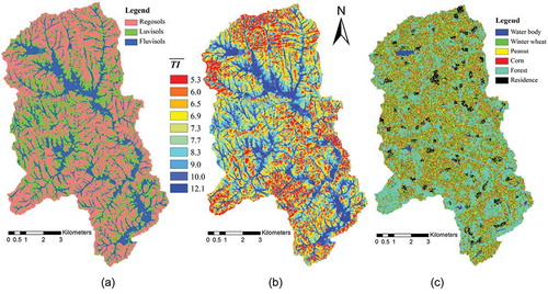
3.2.3 Land-use data

Although the land use is only cropland in the Baocun watershed, the crops vary cyclically because of the crop rotation method with farming three times in every 2 years. Therefore, the average annual land use map is charted to overcome the problem of land utilization change, according to the growth time of crops (Fig. 3(c); Cheng et al. 2014). The property data of crops/vegetation are extracted from the database of SWAT.

3.2.4 Weather data

The daily data (from 1990 to 2013) of the maximum and minimum air temperature, wind speed, relative humidity and solar radiation are collected from three national weather stations (Weihai, Chengshantou and Shidao) located at a distance of about 35 km from the Baocun watershed (black triangles in Fig. 1(a)). The precipitation data are observed at four rainfall gauges during 1990–2013 in the Baocun watershed (circles in Fig. 1(b)). The daily potential evapotranspiration (PET) uses the data measured by pan evaporation equipment at the Baocun hydrometric station (star in Fig. 1(b)).

In this study, the SWAT input-files/input-data of different rainfall–runoff approaches are the same. According to the previous studies (Van Griensven et al. 2006, Güngör and Göncü 2013), 19 key parameters have to be identified by parameter sensitivity analysis, model calibration and validation (Table 1). However, the parameters of surface runoff generation are different among the five rainfall–runoff methods (CN-Soil, CN-ET, G&A, WB and WB-VSA), as detailed in the last column of Table 1. Note that the EDC (Table 1) of the WB approach is defined as the same value in all HRUs to facilitate model calibration, which means the effects of topography on soil saturation deficit are neglected. Because the soil-related parameters of different soil types or layers need to be calibrated independently, resulting in a large number of parameters, the so-called aggregated parameters will be selected instead of the original parameters. In this way, full use can be made of information about spatial variation, the number of parameters can be reduced, and the calibration process simplified (Yang et al. 2007). Aggregated parameters are formed by adding a modification term which includes two types: v__ and r__, referring to a replacement and a relative change to the initial parameter value, respectively (Table 1).

To compare the performances of the five approaches, the river discharge data (1993–2011) are used as a target for model calibration, and the groundwater level data measured in the watershed (cross in Fig. 1(b)) are used for model validation. A warm-up period is recommended by SWAT in order to initialize and then obtain reasonable starting values for model variables. Herein, the warm-up period is from 1990 to 1992, and the model running period for calibration is from 1993 to 2011. The period of model validation using groundwater level data is from June 2007 to December 2011, and the last 2 years (2012 and 2013) of river discharges are also used for model validation.

3.3 Selection of objective functions

There are two widely used criteria of model performance: the coefficient of determination (R²) and the Nash–Sutcliffe efficiency coefficient (NSE) (Nash and Sutcliffe 1970). Because R² is oversensitive to high flow and independent of additive and proportional differences/errors between model simulations and observations, it fails to be used for quantitative assessments of the degree to which the model simulations match the observations (Legates and McCabe 1999, Krause et al. 2005, Criss and Winston 2008). And the NSE also puts greater emphasis on high flow at the expense of the low flow because of the Gaussian error assumption (Cheng et al. 2014). After comparison of many efficiency criteria, Legates and McCabe (1999) found that the mean absolute error (MAE) is slightly preferred over NSE when large outliers (i.e. extreme values) are present, and numerous authors (Krause et al. 2005, Muleta 2012, Wu and Liu 2014) pointed out that the MAE favours balanced consideration of the high and low flows. Furthermore, Criss and Winston (2008) proposed a normalization of MAE, i.e. ‘volumetric’ efficiency (VE), which is calculated by subtracting the ratio between the MAE and the mean of observations from one, to replace NSE:

(14)

where Q_m is the observed river discharge, Q_s is the simulation result, i is the time step.

The VE is dimensionless and ranges from minus infinity to one in theory. If the VE is one, the hydrologic model is perfect. However, if the VE is less than zero, the hydrologic model is no better than a predictor using zeros. In this study, the VE is used as the efficiency criterion for hydrological model assessment.

3.4 Model sensitivity analysis and calibration

The Regional Sensitivity Analysis method with Latin Hypercube Samplings (LHS-RSA) is a method of assessing the sensitivity of model parameters, where the sensitivity is defined as the effect of parameters on overall model performance (Hornberger and Spear 1981, Wagener et al. 2001). The detailed calculation steps are as follows: firstly, use the Latin Hypercube Sampling (LHS) method to generate parameter samplings (40 000 samplings in this study); then substitute these generating parameters into SWAT to obtain the criterion values (VE, equation (14)); next, rank the parameter sets according to the criterion values of VE and separate them into 10 groups in terms of equal sample numbers; finally, calculate the cumulative frequency distribution of each parameter in each group. If a parameter has a significant effect on the model output, there will be a large difference between the cumulative frequency distributions, meaning that the model performance is sensitive to this parameter (Wagener et al. 2001).

To quantify the parameter sensitivity, the proportion of the area enclosed by the envelope curve of cumulative frequency distributions is used as the degree of parameter sensitivity. For example, in Fig. 4, the shadow area is an enclosed area of the envelope curve of cumulative frequency distributions, and the degree of parameter sensitivity is the ratio of the shadow area to the total area. The larger the value of degree, the more sensitive the parameter is.

Figure 4. An example of calculating the degree of parameter sensitivity in the LHS-RSA method.

The DREAM scheme (Vrugt et al. 2009) is used to optimize all parameters in Table 1, because these parameters are all important for river discharges according to previous studies (Van Griensven et al. 2006, Güngör and Göncü 2013), and there are enough data (19 years) for model calibration in this study.

4 Results

4.1 Parameter sensitivity analysis

The LHS-RSA method with the criterion of VE (equation 14) according to the river discharges from 1993 to 2011, is used for the sensitivity analysis of the five rainfall–runoff approaches (CN-Soil, CN-ET, G&A, WB and WB-VSA). As an example, the cumulative frequency distribution analysed by LHS-RSA for the WB-VSA is shown in Fig. 5. In this figure, there are 17 subgraphs corresponding to 17 parameters in the WB-VSA. In each subgraph, the y-axis denotes the cumulative frequency of parameters while the x-axis represents the corresponding parameter values. The 10 lines in the panel are the parameter cumulative frequency distribution of 10 different groups, where the parameter samples are equally divided according to the value of VE and the brightness of line color increases along with the VE increase. The parameters (such as the effective depth of soil profile (EDC), the soil depth (SOL_Z), the soil bulk density (SOL_BD), the soil available water capacity (SOL_AWC), the soil hydraulic conductivity (SOL_K) and the groundwater delay time (GW_DELAY)) show large differences among the cumulative frequency distributions, meaning that these parameters are highly sensitive to the VE with river discharges. Figure 5 also shows that the cumulative frequency distributions for insensitive parameters (such as the plant transpiration (EPCO), the slope roughness (OV_N) and the channel roughness (CH_N1 and CH_N2) for the WB-VSA) are nearly on the same straight line.

Figure 5. Regional sensitivity analysis results for parameters in the WB-VSA approach.

The degree of parameter sensitivity is calculated for the five rainfall–runoff methods and shown in Table 2. In this table, all values are in percentages (%). Comparison of parameter-sensitivity degrees in Table 2 with Fig. 5 reveals that if the degree is less than 4%, the parameter is insensitive to river discharges; by contrast, if the degree is more than 10%, the parameter is significantly sensitive. Comparison of the degrees of parameter sensitivity in Table 2 with different parameters and rainfall–runoff methods indicates parameters of the overland flow generation (such as the curve number (CN2) for CN-Soil, the CN2 and plant evapotranspiration curve number coefficient (CNCOEF) for CN-ET, the SOL_K for G&A and the EDC for WB and WB-VSA) and the soil property parameters (such as SOL_Z, SOL_BD, SOL_K and GW_DELAY) for all approaches are highly sensitive to the VE with river discharges. In contrast, the parameters relating to the evapotranspiration (e.g. EPCO), the overland flow concentration (OV_N and surface flow lag time (SURLAG)), the groundwater revaporization/evaporation (REVAPMN and GW_REVAP), and the channel routing (CH_N1 and CH_N2) are much less sensitive. For the CN-ET, the parameters relating to the water storage and movement of the soil profile and groundwater (such as SOL_Z, SOL_BD, SOL_K and GW_DELAY) are less sensitive than those of other rainfall–runoff approaches.

Table 2. Results of the parameter sensitivity degree (%) for the five rainfall–runoff approaches.

Categories^a	Parameters	CN-Soil	CN-ET	G&A	WB	WB-VSA
Evapotranspiration	v__ESCO	2.61	3.73	3.22	5.03	6.23
	v__EPCO	2.71	5.16	1.87	2.51	2.50
Surface Water	r__CN2	25.44	24.28	2.04	–	–
	v__CNCOEF	–	32.80	–	–	–
	v__EDC	–	–	–	19.83	22.45
	v__OV_N	3.32	4.74	1.77	3.14	3.31
	v__SURLAG	4.39	21.57	1.84	4.74	4.61
Soil water	r__SOL_Z	19.32	14.02	31.84	15.07	16.64
	r__SOL_BD	16.07	8.28	15.59	15.30	16.53
	r__SOL_AWC	9.83	9.94	16.25	9.20	12.10
	r__SOL_K	38.74	22.87	31.37	29.18	31.72
Groundwater	v__GW_DELAY	10.08	7.14	14.21	13.06	12.83
	v__ALPHA_BF	6.25	5.48	6.85	6.56	7.08
	v__GWQMN	6.69	4.57	7.68	5.08	5.87
	v__RCHRG_DP	8.76	7.43	10.12	8.04	7.72
	v__REVAPMN	4.09	4.95	4.84	4.05	4.64
	v__GW_REVAP	3.74	5.42	3.18	3.73	4.52
Tributary/main channel	v__CH_N1	2.81	5.68	2.11	2.70	3.11
	v__CH_N2	3.02	6.00	2.74	2.56	2.40

^aA dash signifies that there are no parameters for this method.

4.2 Model calibration and validation using river discharge data

The parameters optimized by the DREAM with the objective function of VE and the corresponding statistic-measures (VE and NSE) of the hydrologic model performance are listed in Table 3. In this table, the optimized values of most parameters have distinct differences among the five approaches mainly because of the different rainfall–runoff structures. Among the five approaches, the largest value of model efficiency criterion VE is from the simulation of our WB-VSA approach and this highest VE value corresponds to the largest values of NSE as well. It is worth mentioning that the performance of WB-VSA is clearly better than that of widely used CN in model calibration and validation. Compared with the WB, the WB-VSA slightly improves the model performance. By contrast, the G&A and CN-ET approaches based on the infiltration excess or the evaporation-dominant mechanism of rainfall–runoff generation give the poorest results.

Table 3. Optimized parameters for the five rainfall–runoff approaches and performances of the model calibration and validation.

Category	Parameter	CN-Soil	CN-ET	G & A	WB	WB-VSA
Evapotranspiration	v__ESCO	0.515	0.040	0.052	0.468	0.198
	v__EPCO	0.021	0.769	0.991	0.258	0.128
Surface water	r__CN2	−0.394	−0.415	−0.191	―	―
	v__CNCOEF	―	0.192	―	―	―
	v__EDC	―	―	―	0.765	0.781
	v__OV_N	0.351	0.106	0.117	0.404	0.412
	v__SURLAG	0.994	0.510	6.548	1.783	2.550
Soil water	r__SOL_Z	1.403	0.819	0.886	0.865	0.890
	r__SOL_BD	0.835	0.227	0.428	0.354	0.405
	r__SOL_AWC	0.717	1.918	0.004	2.061	1.834
	r__SOL_K	−0.839	−0.311	0.328	−0.185	−0.195
Groundwater	v__GW_DELAY	0.210	0.392	0.373	0.924	0.859
	v__ALPHA_BF	0.182	0.995	0.973	0.970	0.936
	v__GWQMN	297.803	382.189	438.765	582.048	548.907
	v__RCHRG_DP	0.447	0.031	0.001	0.075	0.061
	v__REVAPMN	749.327	829.650	397.525	561.083	527.690
	v__GW_REVAP	0.172	0.060	0.199	0.198	0.183
Tributary/main channel	v__CH_N1	0.047	0.018	0.127	0.006	0.120
	v__CH_N2	0.007	0.056	0.017	0.013	0.031
Model calibration^a	VE^c	0.6071	0.5716	0.5777	0.6059	0.6075
	NSE	0.7992	0.6025	0.6258	0.8188	0.8224
Model validation^b	VE	0.587	0.567	0.577	0.603	0.610
	NSE	0.777	0.686	0.606	0.877	0.879

^aUsing the river discharges from 1993 to 2011.

^bUsing the river discharges in 2012 and 2013.

^cThe efficiency criterion of model calibration.

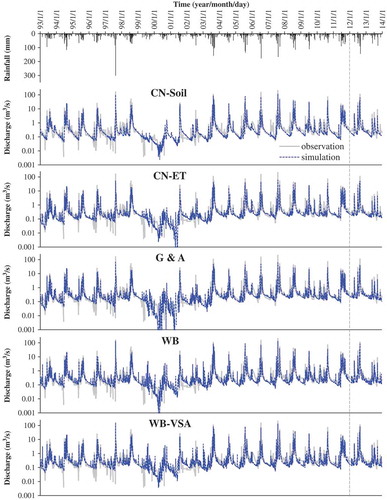
The river discharges from 1993 to 2013 simulated by the five approaches with optimized parameters (Table 3) are shown in Fig. 6. In this figure, the black column (top) is the rainfall, the solid line is the observed river discharge, and the dotted line is the simulated river discharge. Figure 6 shows that all the five rainfall–runoff methods after calibration can reproduce most flood events. However, the CN-Soil, WB and WB-VSA approaches can capture the floods better than the G&A and CN-ET approaches. This is also reflected by the value of NSE: the NSE values of CN-Soil, WB and WB-VSA approaches are obviously greater than those of the G&A and CN-ET approaches. In order to highlight low flow, the observed and simulated river discharges are plotted in Fig. 7 with logarithmic vertical-axes. This figure shows that all the rainfall–runoff approaches, after calibration against observed river discharges, can mimic the low flow well. However, these approaches fail to capture extremely small flow close to zero at the beginning of rainy season, especially in the driest years such as 1999 and 2000, probably because of neglecting the effect of agricultural irrigation on the river discharges during the spring ploughing season in this study. The effect of agricultural irrigation on the river discharges is significant because it (by pumping water from river) often happens before the monsoonal season (about in April; Fig. 6) when the river is dry.

Figure 6. Comparison of the simulated (dotted line) and observed (solid line) river discharges for the five rainfall–runoff approaches.

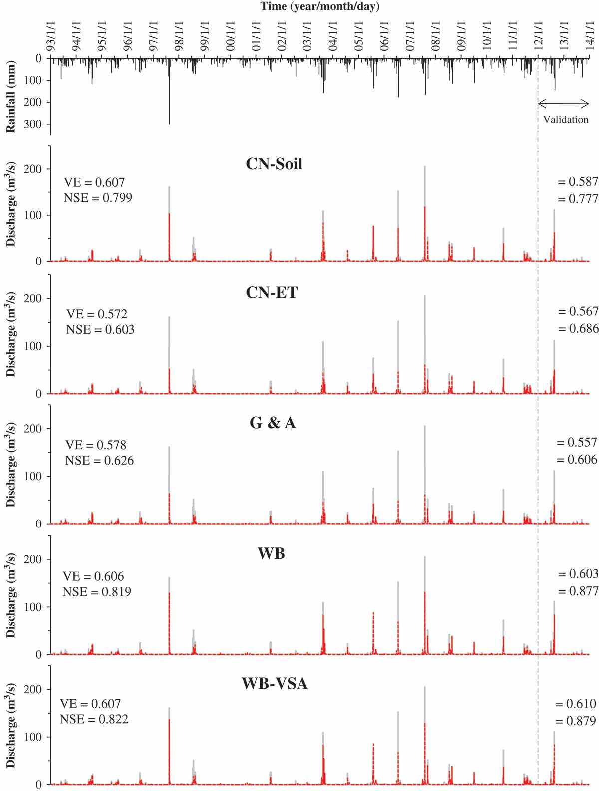
Figure 7. Comparison of the simulated and observed river discharges on the logarithmic vertical-axis (base 10).

Computed by SWAT using the optimized parameters in Table 3, the average annual components of simulated runoff from 1993 to 2011 of the five approaches are listed in Table 4. This table shows that the overland flow substantially differs among the five approaches: the overland flow simulated by the CN-Soil is the largest, which corresponds to the viewpoint of Arnold et al. (2011) that the CN-Soil predicted too many overland runoffs in the shallow-soil area. By contrast, the amount of overland flow is negligible in the CN-ET and G&A approaches. However, the subsurface flow including interflow and groundwater return flow accounts for the larger proportion of runoff components, i.e. 56%, 97%, 100%, 83%, and 83% for CN-Soil, CN-ET, G&A, WB and WB-VSA, respectively. The evapotranspiration is the main method of water loss from the watershed for all five approaches. However, among the five methods, the groundwater losses are different: for the CN-Soil method, the deep recharge is the main method of groundwater loss, whereas the revaporization/evaporation is the main way for three physics-based approaches (G&A, WB and WB_VSA), which better correspond to the characteristics of the shallow-soil area. The groundwater losses of the CN-ET are negligible and the least among the five approaches, but the evapotranspiration is the largest.

Table 4. Comparison of the average annual runoff-components among the five rainfall–runoff approaches.

Categories (mm/a)	CN-Soil	CN-ET	G & A	WB	WB-VSA
Evapotranspiration	490.3	539.5	476.1	476.8	485.3
Overland flow	112.38	7.5	0.0	44.35	45.74
Lateral flow	62.92	91.04	119.27	117.76	119.92
Baseflow	82.27	155.82	134.76	106.25	104.63
Revaporization^a	0.0	0.0	79.34	50.99	45.29
Deep recharge^b	68.37	5.17	0.22	13.6	10.37

^aThe evaporation of groundwater.

^bThe groundwater losses from the shallow aquifer to the deep aquifer.

4.3 Model validation using groundwater data

In each HRU, SWAT separately simulates the soil water of the soil profile and the groundwater of shallow aquifer, and neglects the interactions between soil water and groundwater (Fig. 2). Therefore, SWAT fails to mimic the groundwater table level directly. Vazquez-Amábile and Engel (2005) and White et al. (2011) proposed a method that converts the model-predicted/simulated soil water to an equivalent groundwater depth by dividing by soil porosity. This method depends heavily on the measurement precision of soil porosity. However, it is difficult or impossible to accurately measure soil porosity in the field because of its heterogeneity.

As shown in Fig. 1(b), the groundwater gauge in the Baocun watershed is located in the flood plain and started working in June 2007. The borehole material shows that the soil can be separated into three layers: (i) 0.0–1.5 m, filled with loose soil, (ii) 1.5–3.5 m, silty and coarse sand, and (iii) below 3.5 m, coarse sand. The average groundwater table depth is 2 m, and the groundwater table depth varies between 0.8 m and 3.5 m during the monitoring period. Because of the shallow water table depth and the sandy soil layers with high hydraulic conductivity around the groundwater gauge, the storage capacity of the unsaturated soil layer could be neglected on the daily time step. As a result, the groundwater level can reflect the amount of soil water (Qiao et al. 2013). In other words, there is a linear relationship between the groundwater table level and the total soil water volume. The slope of the linear relationship approximates the specific yield of the unconfined aquifer (Cheng et al. 2014).

SWAT can predict the total soil water amount by adding the soil water in the soil profile and the groundwater in the shallow aquifer. Therefore, in order to avoid measuring soil porosity, we directly tested the linear relationship between the observed groundwater level and the simulated soil water volume stored in the soil profile and shallow aquifer of the HRU that the groundwater gauge fell into, for model validation. Comparisons of observed groundwater level and simulated soil water volume among the five rainfall–runoff approaches are presented in Fig. 8. The performance indicator is the coefficient of determination (R²), which reflects the linear correlation between the observed groundwater level and the simulated soil water volume.

Figure 8. Observed groundwater levels versus simulated soil water volume of the five rainfall–runoff approaches.

Figure 8 demonstrates the empirical rainfall–runoff approach of CN-Soil simulates the groundwater levels worst. Even the R² of the CN-ET (in which the surface runoff generation is independent of soil water content) is better than that of CN-Soil. By contrast, the physics-based rainfall–runoff approach WB-VSA proposed in this study mimics the groundwater levels best.

5 Discussion

5.1 Parameter characteristics

After comparison of the parameter sensitivity of SWAT among many watersheds, Van Griensven et al. (2006) pointed out that there were distinct differences in sensitivity results between different watersheds because the effect of the parameters on model performance depends on watershed characteristics such as land use, topography and soil types. Therefore, parameter sensitivity results in this study may be different from other studies, e.g. the parameters of soil properties (such as soil depth (SOL_Z) and hydraulic conductivity (SOL_K)) in this study are more sensitive than those in the study of Van Griensven et al. (2006). And the parameter sensitivity results reflect the characteristics of the Baocun watershed and the rainfall–runoff approaches.

In this study, the parameters relating to the overland flow generation and the soil water storage and movement are all highly sensitive in the five rainfall–runoff approaches (Table 2). Correlatively, the proportions of subsurface flow are all large (Table 4), and the rainfall–runoff approaches all well mimic the baseflow (Fig. 7). This may result for three reasons: (1) the model efficiency criterion VE can balance consideration of the high and low flow (Krause et al. 2005, Muleta 2012, Wu and Liu 2014); (2) the calculation methods for subsurface flow are the same among the five rainfall–runoff approaches (Neitsch et al. 2005, White et al. 2011); (3) there is a lot of low flow and considerable temporal variance of the river discharges in the Baocun watershed, where the proportion of flow less than 1.0 m³/s accounts for 89% of total records, the proportion of zero-flow reaches 10% and the mean of daily river discharges is only 0.8 m³/s, but the standard deviation is 4.8 m³/s and the maximum value reached 205 m³/s in 2007 (Fig. 6). In short, the main reason may be that the model efficiency criterion VE puts greater emphasis on the low flow in Baocun watershed (Cheng et al. 2014). By contrast, because of the small flood-concentration time (less than 2 hours) in the Baocun watershed, the parameters relating to overland runoff concentration and channel routing are less sensitive (Table 2; Cheng et al. 2014).

The CN-ET uses the potential evaporation to estimate the retention parameter (equation (4)) which weakens the interactions between surface flow parameters and soil parameters. Therefore, its parameters relating to soil properties are less sensitive than those of other rainfall–runoff approaches (Table 2) and its evapotranspiration is the largest (Table 4).

5.2 Simulation results

The field survey results show that the Baocun watershed was intensively affected by human activities and the whole watershed was terraced for agriculture even at the mountaintop where the steep slopes were transformed to staircase platforms. The terraced fields can delay the overland flow and facilitate the rainfall infiltration. As a result, there is a lot of low flow and no surface runoff generation until the soil layer is saturated in the Baocun watershed, although it is a mountain watershed with a shallow soil layer. In addition, there is abundant rainfall (806 mm/year). Therefore, the saturation excess overland flow method may be more appropriate for the Baocun watershed than the infiltration excess overland flow method, which was confirmed by the results of model performance (Table 3): the model performance indicators (VE and NSE) of the water balance methods (WB-VSA and WB) are much better than those of the G&A approach which uses the Green-Ampt equation to estimate the soil infiltration capacity (equation (7)). It is actually because the NSE always puts emphasis on the high flow (Cheng et al. 2014) that the flood simulation results of the water balance methods (WB-VSA and WB) are much better than that of the G&A method (Table 4; Fig. 6). The very large soil hydraulic conductivity (SOL_K) inferred by the automatic optimization program with the G&A approach (Table 3) results in the very large soil infiltration capacity and no infiltration excess overland flow occurring (Table 4; Kannan et al. 2007).

Because the CN-Soil approach implies the principle of saturation excess overland flow (Steenhuis et al. 1995), it gets similar model performance for river discharges to the water balance methods (WB-VSA and WB) in the Baocun watershed (Table 3). However, CN-Soil is an empirical method that assumes two empirical relationships: one between the retention (rainfall not converted into runoff) and runoff properties of the watershed and the rainfall (equation (1)), and the other between the retention parameter and the soil water content (equation (3)), so it mimics the groundwater levels worst (Fig. 8). Surprisingly, the groundwater simulation results of the CN-ET approach are much better than those of CN-Soil (Fig. 8), although the two approaches are all based on the CN method. This may result for two reasons: (1) the CN-ET simulates the surface flow and the subsurface flow separately, because the retention parameter of CN-ET is estimated by the potential evaporation, rather than the soil water content (equation (4)); and (2) the automatic optimization program with the VE makes the CN-ET mimic the baseflow well (Fig. 7). For these reasons, the flood simulation results of the CN-ET approach are much worse than those of the CN-Soil approach (Tables 3 and 4; Fig. 6).

The TOPMODEL under the steady-state condition and exponential decline of transmissivity with depth assumptions has been widely accepted by hydrologists (Beven 1997). Its key contribution is building a linear relationship between the soil moisture deficit and the topographic index (Beven 1997). In the WB, White et al. (2011) introduced a parameter (EDC) to reflect the effect of topography on soil moisture deficit. The WB-VSA further improved WB by transplanting the linear expression of soil moisture deficit in the TOPMODEL to the EDC in WB. However, in the Baocun watershed, because the terraced fields change the micro-topography and weaken the effects of topography on soil saturation deficit, the effective soil depth is close to the original soil depth (i.e. the value of EDC is close to 1.0) in both WB and WB-VSA (Table 3; equation (10)). The relationship between the value of EDC and the topographic index is shown in Fig. 9. This figure shows that the EDC in the WB looks like the average value of the EDC_i in the WB-VSA. Consequently, the river discharge simulation results of the WB-VSA only improved a little compared with the WB (Table 3). However, some other factors still confirmed the theory of the WB-VSA: first, the EDC as the catchment average EDC_i in the WB-VSA (equation (13)) approximates to the constant EDC of all HRUs assumed by the WB (Table 3; Fig. 9). In other words, the WB is only a special case of the WB-VSA in the Baocun watershed because of the small effects of topography on soil saturation deficit. Second, the groundwater simulation result of the WB-VSA is obviously better than that of the WB (Fig. 8), which means that WB-VSA better reflects the spatial variation of runoff generation.

Figure 9. The value of EDC as a function of topographic index in the WB-VSA and WB approaches.

6 Conclusions

In this study, the sensitivity analysis, calibration and validation procedures were performed for the WB-VSA approach developed by this study and for the other four methods of CN-Soil, CN-ET, G&A and WB for comparison purposes. In order to balance consideration of the high and low flow, the VE was used as the model efficiency criterion. The results of parameter sensitivity and runoff component analysis demonstrate that the VE with discharges is sensitive to the greatest number of parameters (especially the overland flow generation and soil property parameters) of the five rainfall–runoff approaches, and the subsurface flow controls river discharge variations in the rainfall–runoff simulation for the Baocun watershed possibly because of the effects of human activities especially terraced fields.

The results of model calibration with river discharges and model validation with groundwater levels demonstrate that WB-VSA is the most accurate in simulating flow discharge and groundwater owing to reflection of the spatial variation of runoff generation affected by topography and soil properties. The WB and CN-Soil approaches also mimic the river discharges well with the consideration of the principle of saturation excess overland flow. In contrast, the flood simulation results of the G&A based on Horton overland flow and the CN-ET that neglects the relationship between the surface flow generation and the soil water content are much worse. However, the groundwater simulation results of the empirical method (CN-Soil) are the worst. By comparison, the WB-VSA as a physics-based methods best mimics the groundwater levels.

The WB-VSA approach established a linear relationship between the EDC and the TI by reference to the principle of TOPMODEL. Compared with the WB, the WB-VSA improves both the simulation results of river discharges and groundwater levels. On the other hand, because the terraced fields change the micro-topography and weaken the effects of topography on soil saturation deficit in the Baocun watershed, the effective soil depth in both WB and WB-VSA is close to the original soil depth, and the WB becomes a special case of the WB-VSA, of which the optimization parameters and simulation results are similar to that of the WB-VSA.

Acknowledgements

The authors would like to thank Weihai Hydrology and Water Resource Survey Bureau for providing hydrologic data, the National Meteorological Information Center, China Meteorological Administration (CMA) for providing climate data, and the computing facilities of Freie Universität Berlin (ZEDAT) for computer time. The authors also wish to thank two anonymous reviewers for their valuable comments that led to significant improvements in the paper.

Disclosure statement

No potential conflict of interest was reported by the author(s).

Additional information

Funding

This research was supported by the National Natural Science Foundation of China (No. 51190091), the International Science & Technology Cooperation Program of China (No. 2012DFG22140), the Fundamental Research Funds for the Central Universities (No. B15020003), the Natural Science Foundation of Jiangsu Province, China (No. BK20150809) and a governmental scholarship from the China Scholarship Council (CSC).

References

- Arnold, J.G., et al., 2011. Soil and water assessment tool input/output file documentation version 2009. College Station, TX: Texas Water Resources Institute Technical Report, No. 365.
- Beven, K., 1997. TOPMODEL: a critique. Hydrological Processes, 11 (9), 1069–1085. doi:10.1002/(ISSN)1099-1085
- Beven, K., Gilman, K., and Newson, M., 1979. Flow and flow routing in upland channel networks. Hydrological Sciences Bulletin, 24, 303–325. doi:10.1080/02626667909491869
- Chen, X., et al., 2010. Simulating the integrated effects of topography and soil properties on runoff generation in hilly forested catchments, South China. Hydrological Processes, 24 (6), 714–725. doi:10.1002/hyp.7509
- Cheng, Q.-B., et al., 2011. Water infiltration underneath single-ring permeameters and hydraulic conductivity determination. Journal of Hydrology, 398, 135–143. doi:10.1016/j.jhydrol.2010.12.017
- Cheng, Q.-B., et al., 2014. Improvement and comparison of likelihood functions for model calibration and parameter uncertainty analysis within a Markov chain Monte Carlo scheme. Journal of Hydrology, 519 (27), 2202–2214. doi:10.1016/j.jhydrol.2014.10.008
- Criss, R.E. and Winston, W.E., 2008. Do nash values have value? Discussion and alternate proposals. Hydrological Processes, 22, 2723–2725. doi:10.1002/hyp.v22:14
- Dunne, T., 1978. Field studies of hillslope flow processes. In: M.J. Kirkby, ed. Hillslope hydrology. Chichester: Wiley.
- Easton, Z.M., et al., 2008. Re-conceptualizing the Soil and Water Assessment Tool (SWAT) model to predict runoff from variable source areas. Journal of Hydrology, 348 (3–4), 279–291. doi:10.1016/j.jhydrol.2007.10.008
- Easton, Z.M., et al., 2011. A simple concept for calibrating runoff thresholds in quasi-distributed variable source area watershed models. Hydrological Processes, 25, 3131–3143. doi:10.1002/hyp.v25.20
- Ficklin, D.L. and Zhang, M., 2013. A comparison of the curve number and green-ampt models in an agricultural watershed. Transactions of the ASABE, 56 (1), 61–69. doi:10.13031/2013.42590
- Gabellani, S., et al., 2008. General calibration methodology for a combined Horton-SCS infiltration scheme in flash flood modeling. Natural Hazards and Earth System Sciences, 8, 1317–1327. doi:10.5194/nhess-8-1317-2008
- Garen, D.C. and Moore, D.S., 2005. Curve number hydrology in water quality modeling: uses, abuses and future directions. Journal of the American Water Resources Association, 41, 377–388. doi:10.1111/jawr.2005.41.issue-2
- Gassman, P.W., et al., 2007. The soil and water assessment tool: historical development, applications, and future research directions. American Society of Agricultural and Biological Engineers, 50 (4), 1211–1250.
- Grimaldi, S., Petroselli, A., and Romano, N., 2013. Green-Ampt Curve-Number mixed procedure as an empirical tool for rainfall–runoff modelling in small and ungauged basins. Hydrological Processes, 27 (8), 1253–1264. doi:10.1002/hyp.9303
- Güngör, Ö. and Göncü, S., 2013. Application of the soil and water assessment tool model on the lower porsuk stream watershed. Hydrological Processes, 27, 453–466. doi:10.1002/hyp.v27.3
- Han, E., Merwade, V., and Heathman, G.C., 2012. Implementation of surface soil moisture data assimilation with watershed scale distributed hydrological model. Journal of Hydrology, 416–417, 98–117. doi:10.1016/j.jhydrol.2011.11.039
- Hornberger, G.M. and Spear, R.C., 1981. An approach to the preliminary analysis of environmental systems. Journal of Environmental Management, 12, 7–18.
- Jeong, J., et al., 2010. Development and integration of sub-hourly rainfall–runoff modeling capability within a watershed model. Water Resources Management, 24 (15), 4505–4527. doi:10.1007/s11269-010-9670-4
- Kannan, N., et al., 2007. Sensitivity analysis and identification of the best evapotranspiration and runoff options for hydrological modelling in SWAT-2000. Journal of Hydrology, 332 (3–4), 456–466. doi:10.1016/j.jhydrol.2006.08.001
- King, K.W., Arnold, J.G., and Bingner, R.L., 1999. Comparison of Green – Ampt and curve number methods on Goodwin Creek watershed using SWAT. American Society of Agricultural Engineers, 42 (4), 919–926. doi:10.13031/2013.13272
- Krause, P., Boyle, D.P., and Bäse, F., 2005. Comparison of different efficiency criteria for hydrological model assessment. Advances in Geosciences, 5, 89–97. doi:10.5194/adgeo-5-89-2005
- Legates, D.R. and McCabe Jr., G.J., 1999. Evaluating the use of “goodness-of-fit” measures in hydrologic and hydroclimatic model validation. Water Resources Researches, 35 (1), 233–241. doi:10.1029/1998WR900018
- Loague, K., et al., 2010. The quixotic search for a comprehensive understanding of hydrologic response at the surface: Horton, Dunne, Dunton and the role of concept-development simulation. Hydrological Processes, 24, 2499–2505.
- Lyon, S.W., et al., 2004. Using a topographic index to distribute variable source area runoff predicted with the SCS curve-number equation. Hydrological Processes, 18, 2757–2771. doi:10.1002/hyp.1494
- Migliaccio, K.W. and Srivastava, P., 2007. Hydrologic components of watershed-scale models. Transactions of the ASABE, 50 (5), 1695–1703. doi:10.13031/2013.23955
- Mishra, S.K. and Singh, V.P., 2003. Soil conservation service curve number (SCS-CN) methodology. Dordrecht, Netherlands: Kluwer Academic Publishers.
- Muleta, M. K., 2012. Model performance sensitivity to objective function during automated calibrations. Journal of Hydrologic Engineering, 17 (6), 756–767. doi:10.1061/(ASCE)HE.1943-5584.0000497
- Nash, J.E. and Sutcliffe, J.V., 1970. River flow forecasting through conceptual models 1: A discussion of principles. Journal of Hydrology, 10 (3), 282–290. doi:10.1016/0022-1694(70)90255-6
- Neitsch, S.L., et al., 2005. Soil and water assessment tool theoretical documentation and user’s manual, version 2005. Temple, TX: GSWR Agricultural Research Service & Texas Agricultural Experiment Station.
- Ponce, V.M. and Hawkins, R.H., 1996. Runoff curve number: has it reached maturity? Journal of Hydrologic Engineering, 1 (1), 11–19. doi:10.1061/(ASCE)1084-0699(1996)1:1(11)
- Qiao, L., Herrmann, R.B., and Pan, Z.-T., 2013. Parameter uncertainty reducition for SWAT using grace, streamflow, and groundwater table data for lower Missiouri river basin. JAWRA Journal of the American Water Resources Association, 49 (2), 343–358. doi:10.1111/jawr.2013.49.issue-2
- Rallison, R.E. and Miller, N., 1982. Past, present, and future SCS runoff procedure. In: V.P. Singh, ed. Rainfall–runoff relationship. Littleton, CO: Water Resources Publications, 353–364.
- Schneiderman, E.M., et al., 2007. Incorporating variable source area hydrology into a curve-number-based watershed model. Hydrological Processes, 21, 3420–3430. doi:10.1002/(ISSN)1099-1085
- SCS, 1972. SCS national engineering handbook, Section 4. Washington, DC: Hydrology, Soil Conservation Service, US Department of Agriculture.
- Steenhuis, T., et al., 1995. SCS runoff equation revisited for variable-source runoff areas. Journal of Irrigation and Drainage Engineering, 121 (3), 234–238. doi:10.1061/(ASCE)0733-9437(1995)121:3(234)
- Tedela, N.H., et al., 2012. Runoff curve numbers for 10 small forested watersheds in the mountains of the eastern United States. Journal of Hydrologic Engineering, 17 (11), 1188–1198. doi:10.1061/(ASCE)HE.1943-5584.0000436
- Van Griensven, A., et al., 2006. A global sensitivity analysis tool for the parameters of multi‐variable catchment models. Journal of Hydrology, 324 (1–4), 10–23. doi:10.1016/j.jhydrol.2005.09.008
- Vazquez-Amábile, G.G. and Engel, B.A., 2005. Use of SWAT to compute groundwater table depth and streamflow in the Muscatatuck River watershed. Transactions of the ASABE, 48 (3), 991–1003. doi:10.13031/2013.18511
- Vrugt, J.A., et al., 2009. Accelerating Markov chain Monte Carlo simulation by differential evolution with self-adaptive randomized subspace sampling. International Journal of Nonlinear Sciences and Numerical Simulation, 10 (3), 273–290. doi:10.1515/IJNSNS.2009.10.3.273
- Wagener, T., et al., 2001. A framework for development and application of hydrological models. Hydrology and Earth System Sciences, 5 (1), 13–26. doi:10.5194/hess-5-13-2001
- Walter, M.T. and Shaw, S.B., 2005. Discussion: ‘‘Curve number hydrology in water quality modeling: uses, abuses, and future directions’’ by Garen and Moore. Journal of the American Water Resources Association, 41 (6), 1491–1492. doi:10.1111/jawr.2005.41.issue-6
- Wang, L., Song, M., and Wang, P., 2002. Study development on Jiaonan - Weihai tectonic belt and discussion of some important geological problems. Geology of Shandong, 18 (3–4), 78–83. (in Chinese).
- White, E.D., et al., 2011. Development and application of a physically based landscape water balance in the SWAT model. Hydrological Processes, 25, 915–925. doi:10.1002/hyp.v25.6
- Wu, Y. and Liu, S., 2014. A suggestion for computing objective function in model calibration. Ecological Informatics, 24, 107–111. doi:10.1016/j.ecoinf.2014.08.002
- Yang, J., et al., 2007. Hydrological modelling of the Chaohe Basin in China: statistical model formulation and Bayesian inference. Journal of Hydrology, 340, 167–182. doi:10.1016/j.jhydrol.2007.04.006
- Yu, B.-F., 1998. Theoretical Justification of SCS method for runoff estimation. Journal of Irrigation and Drainage Engineering, 124, 306–310. doi:10.1061/(ASCE)0733-9437(1998)124:6(306)
- Yu, B.-F., 2012. Validation of SCS method for runoff estimation. Journal of Hydrologic Engineering, 17 (11), 1158–1163. doi:10.1061/(ASCE)HE.1943-5584.0000484
- Yuan, Y., et al., 2001. Modified SCS curve number method for predicting subsurface drainage flow. Transactions of the ASABE, 44 (6), 1673–1682.