Robust flood statistics: comparison of peak over threshold approaches based on monthly maxima and TL-moments

ABSTRACT

Flood quantile estimation based on partial duration series (peak over threshold, POT) represents a noteworthy alternative to the classical annual maximum approach since it enlarges the available information spectrum. Here the POT approach is discussed with reference to its benefits in increasing the robustness of flood quantile estimations. The classical POT approach is based on a Poisson distribution for the annual number of exceedences, although this can be questionable in some cases. Therefore, the Poisson distribution is compared with two other distributions (binomial and Gumbel-Schelling). The results show that only rarely is there a difference from the Poisson distribution. In the second part we investigate the robustness of flood quantiles derived from different approaches in the sense of their temporal stability against the occurrence of extreme events. Besides the classical approach using annual maxima series (AMS) with the generalized extreme value distribution and different parameter estimation methods, two different applications of POT are tested. Both are based on monthly maxima above a threshold, but one also uses trimmed L-moments (TL-moments). It is shown how quantile estimations based on this “robust” POT approach (rPOT) become more robust than AMS-based methods, even in the case of occasional extraordinary extreme events.

Editor M.C. Acreman Associate editor A. Viglione

KEYWORDS:

• partial duration
• annual maxima
• robustness
• Poisson process

1 Introduction

The estimation of flood quantiles with very low exceedence probabilities is a key problem of engineering hydrology. Since the recorded series of floods are very limited in number and seldom longer than 100 years, the probabilities of extreme flood events needed are derived from a fitting of a suitable distribution function and its extrapolation into the realm of very low exceedence probabilities. The selection of the underlying statistical model is crucial in this context. One problem of this common approach consists in the temporal variability of statistical characteristics of these series, which results from exceptional extreme events happening occasionally. Those events modify the parameters of distribution functions and their quantiles temporally. The impact of this temporal variability is aggravated if the demand for design floods increases after disastrous flood events, which often results in step changes of the parameters of distribution functions. In many cases, such changes are smoothed again by subsequent periods of “normal” floods. Fig. 1 shows an example of step-wise changes of the 99% quantile derived from the generalized extreme value (GEV) distribution with probability-weighted moments and a year-by-year extended flood series. If these quantiles are applied for design of long-lasting hydraulic structures, their temporal variability becomes a problem.

Figure 1. Annual maxima for the Wechselburg gauge (1910–2013) and the estimated 99% quantile for increasing sample length.

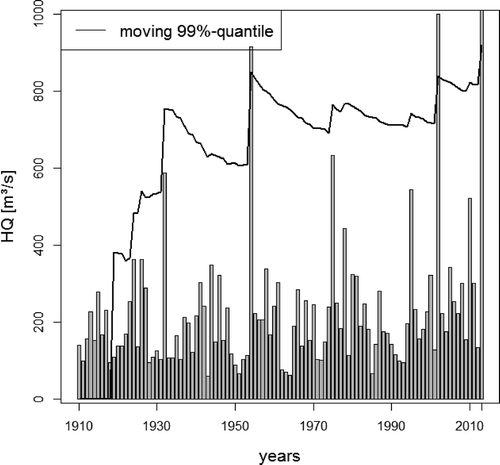
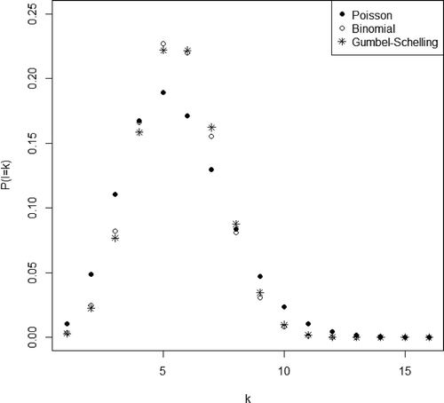
Figure 2. Differences between the discrete distribution functions of the number of exceedences for the Nossen gauge.

There are several approaches to handling such extraordinary events, which cause step changes in hydrological parameters and quantiles. One of them consists in detection and removal of outliers. An outlier is an observation that deviates markedly from the other observations in the sample. Several procedures exist for determining statistically whether the highest observations in the sample are statistical outliers. For example, the widely used Grubbs test is recommended when testing for a single outlier (Grubbs 1969). The generalized extreme Studentized deviate (ESD) proposed by Rosner (1983) can be applied when the exact number of multiple outliers is not known. Such statistical tests were developed to identify which extreme events can be considered to be unexpected. The level of expectation depends on the assumption of the underlying distribution of the data. Often it is assumed that the data follow an approximately normal distribution, but tests for the detection of outliers in data with other underlying distributions also exist (e.g. Spencer and McCuen 1996).

If an outlier is detected, the question arises how to handle it. The outlier could be an erroneous value, which should be corrected or removed. Outliers in flood statistics may be the result of a mixed population occurrence (Klemeš 1986). If we exclude these two possibilities, we can conclude that it is just an event from the tail of the distribution. Here we have two options: it could be censored to avoid distorting the analyses, or it could be used with a weighting to minimize the resulting distortion. The latter option became very popular by introducing L-moments, which are relatively robust to the effects of outliers (Hosking 1990), or LH-moments (Wang 1997), a generalization of L-moments, for characterizing the upper part of distributions and larger events in data.

Another option to obtain more robust estimations of quantiles is trimming. In contrast to censoring, extreme values are excluded without taking into account their frequencies. An overview of the effect of trimming on log-Pearson type III quantile estimates is given by Ouarda and Ashkar (1998). These authors discuss the potential usefulness of robust estimators but also demonstrate the risk of overly robust quantile estimations. Trimmed L-moments, defined by Elamir and Seheult (2003), are useful for distributions with very heavy tails to provide measures analogous to L-moments that remain meaningful for distributions, where the mean does not exist (Hosking 2007). These are mostly very heavy tailed distributions, for example the Cauchy distribution.

The question arises which methodological options exist to specify a more robust estimation of flood peaks with low probabilities but avoiding overly robust quantile estimations. The methods described below are applied to compare the robustness of their results.

As the classical model for annual maxima series (AMS), we chose the GEV distribution. The parameters are estimated with two different methods, maximum likelihood (ML) and probability weighted moments (PWM). The ML estimators are known to be quite efficient but difficult to calculate, needing numerical solutions. The PWM (Greenwood et al. 1979) are a more robust extension of the classical product moments and, unlike these, they exist for all possible values of the shape parameter (Kumar et al. 1994). For small and moderate sample sizes (up to n = 100), they have a smaller or similar variance as the ML-estimates (Hosking et al. 1985, Madsen et al. 1997).

It is known that the partial duration series (peak over threshold (POT) approach) constitutes an important alternative to the classical AMS in performing flood frequency analysis. It has been argued that the POT approach uses more data and thus more information about the floods, whereas AMS only uses one event per year and therefore ignores other floods in the same year that are higher than the annual maxima in other years. Therefore, it is likely that the POT has a more robust behaviour. For the parameter estimation we used PWM. We also used the POT approach with trimmed L-moments (TL-moments) (rPOT).

The return periods derived from annual series are annual occurrences, whereas the return periods of POT are time spans between exceedences of the threshold. Comparisons of the statistics of time periods between flood events derived from partial duration series and annual series are given by Langbein (1949) and Stedinger et al. (1993). They show that for return periods higher than 10 years it makes no difference which approach is used. Nevertheless, we will see that it makes a difference with respect to robustness if we calculate annual return period based on AMS or based on the partial series. Additionally, Cunnane (1973), Rosbjerg (1985) and Madsen et al. (1997) compare the efficiency of the estimation of annual return periods by the annual maxima and partial duration series for independent and dependent peaks and different estimators. Also, Tavares and Da Silva (1983) show the differences in the estimation variance of both cases. Rasmussen and Rosbjerg (1991) considered seasonal approaches for the partial duration series.

In the following, we compare the classical statistics of annual maxima with the annual maximum statistic resulting from the two POT approaches with respect to its robustness. In particular, we want to estimate extreme quantiles (99% and 99.5%) of different gauges within a river basin (the Mulde basin in Saxony, Germany). Several extreme events happened in this basin in the last 12 years, so we can find several extraordinary floods in our data samples. Robustness in this context means stability of the quantiles against the occurrence of extreme events.

The paper is organized as follows. In Section 2 the POT and rPOT approaches are described. The probability distributions, which are based on POT, are a combination of two distribution functions: one for the magnitude of exceedences, the other for the annual number of exceedences (the latter a discrete distribution). We investigate the influence of the choice of the discrete distribution for POT. Often the Poisson distribution is applied for this purpose. This choice is based on the assumption of an underlying Poisson process. Nevertheless, it can be shown that it is not the best fitting distribution in some cases. Extending the study of Önöz and Bayazit (2001), we replace it by other discrete distributions, especially one proposed by Gumbel and Schelling (1950). Some practical aspects of their application are discussed. In Section 3 we specify hydrological metrics for the robustness of flood quantiles. These are applied in Section 4 to assess the performance of POT and rPOT in a German case study. In Section 5 we summarize the main conclusions.

2 Methods

2.1 Conventional methods

Flood statistics are mostly based on annual maxima series (AMS). The estimation of distribution functions can be done with the method of moments, the maximum likelihood method or probability weighted moments (Hosking et al. 1985). Here, we applied these three methods to adapt the GEV to flood series. In a number of European countries, the GEV is among the recommended choices of distribution functions (Salinas et al. 2014). It is also the preferred distribution in our region of interest. The GEV was also selected here, as the Fisher-Tippet-Gnedenko theorem (Fisher and Tippett 1928) says that for independent, identically distributed random variables the maximum (properly normalized) converges in distribution to a GEV distribution (under some technical conditions) for . In this theorem the normalizing factors for the maximum ensure a convergence of the normalized maximum to a non-degenerate random variable with an extreme value distribution. In hydrology, this limit distribution is widely known and often applied (see NERC 1975, Hosking et al. 1985) because of the flexibility of the distribution function with three parameters:

(1)

for , where is the shape parameter, the scale parameter and the location parameter. The special case is called the Gumbel distribution and is given by:

(2)

It is not necessary to normalize the given data since an asymptotic convergence to a non-degenerate random variable can be assumed.

The GEV with the various parameter estimation methods forms the benchmark to specify more robust estimations of flood quantiles. To differentiate from the POT approach that we apply, we use the abbreviation AMS when we fit a GEV to the annual maxima series and refer to the parameterization used when it is necessary.

2.2 POT models

In comparison to AMS, the POT method enlarges the information used for the fitting by considering not only the annual maxima but every (in our case monthly) maximum of discharge above a threshold, specifying a flood. Let us consider a data set with , that is, for example, an n = 100-year series of d = 12 monthly maximum discharges in a year. Of course, this model could also be applied with other numbers of realisations d per year. It is important to consider that not every monthly maximum specifies a flood peak, which has to be specified by a threshold. Since we are interested in flood statistics, we have to exclude such monthly maxima, which are not related to floods, to avoid average or low discharges influencing the flood statistics. For threshold we use the minimum of the series of annual maxima to obtain a partial duration series. Also, the independence between the single flood events has to be ensured. Here we applied an approach, suggested by Malamud and Turcotte (2006), where a minimum time between two flood peaks is required to specify two independent flood events. For the watersheds in our data application with areas of several hundred square kilometres, we use a time span of at least 7 days.

For application of POT we use a theorem of the extreme value theory to find a suitable distribution, the Balkema-de Haan-Pickands theorem (Balkema and de Haan 1974, Pickands 1975). It says that the conditional excess distribution of above a certain threshold converges to a generalized Pareto distribution (GPD) with distribution function:

(3)

for x > if the shape parameter is , and otherwise, and the scale parameter .

For the conditional excess distribution, many other distribution functions can be used, especially the special case of the GPD, which is called the shifted exponential distribution:

(4)

Rosbjerg et al. (1992) have shown that this distribution is preferable in the case where , as it gives a better approximation to the data. Nevertheless, to ensure a high degree of flexibility, we apply the three-parametric case, which can be reduced to the special case of the exponential distribution.

Here the threshold parameter is given by definition and does not have to be estimated. However, it is essential to mention that the choice of it plays an important role in the behaviour of the estimates (see Beguería 2005). As we are interested in annual return periods, one problem remains. We have to transform the results we get from the GPD, the distribution of the magnitude of excesses, into annual return periods. The relationship between annual maxima and the partial duration series can be specified as follows. Using the total probability theorem, we obtain for the distribution function of the annual maxima F_a (see Shane and Lynn 1964):

(5)

where is the probability that the annual number of exceedences of equals k.

The most popular discrete distribution for describing the occurrence of rare events is the Poisson distribution:

(6)

based on the assumption that the underlying process is a Poisson process. Therefore, it seems natural to use this distribution also in the case of the annual number of exceedences, and actually this is done in most cases (e.g. Cunnane 1973, Rosbjerg 1985, Stedinger et al. 1993). The parameter represents both the mean and the variance of the distribution and is estimated by the mean of the annual number of exceedences:

(7)

Nevertheless, the application of the Poisson distribution also has some disadvantages in the case of partial duration series. One important point is that equation (5) specifies probability mass for every k = 0,1,…, even for k > d. Having in mind the example of d = 12 monthly maxima every year, it is not possible that would be exceeded more than 12 times per year. Another problem, which has been discussed in the literature, is the assumption of equal mean and variance, which is the base of the Poisson distribution, but this does not always hold (Taesombut and Yevjevich 1978, Cunnane 1979, Önöz and Bayazit 2001). For this reason we consider different distributions and compare the results. Mathematically, the binomial distribution is applicable since it is a typical distribution for describing the number of exceedences of a threshold in a sample (Önöz and Bayazit 2001). Its probability mass function is given by:

(8)

where p is the probability of an exceedence of the threshold and is estimated as:

(9)

By choosing r = d we avoid the problem of having probability mass for k > d, since then the binomial distribution function equals 0. The binomial distribution converges to the Poisson distribution for and with .

As the third and last distribution, we use a distribution proposed by Gumbel and Schelling (1950):

(10)

where m is the rank of in the sample in decreasing order.

If and , Gumbel and Schelling (1950) have shown that this distribution converges asymptotically to a normal distribution; otherwise, if and m and k remain small, it converges to the Poisson distribution. This distribution has the advantage that we do not have to estimate any parameters and therefore have no uncertainties at this point. The only assumption needed is continuity of the data. The differences among these three distributions are shown by the example of a German flood series (Fig. 2) The Poisson distribution has a broader but flatter behaviour, with probability mass even for k > 12, that is, monthly maximum discharges exceeding a threshold more than 12 times a year. The binomial and Gumbel-Schelling distributions have similar behaviour, although the Gumbel-Schelling distribution has greater skewness. The influence of the different shapes was examined by comparing the three different POT models (Poisson, binomial and Gumbel-Schelling) via their quantiles. The results are similar to those of Önöz and Bayazit (2001). The influence of the chosen weighting distribution is negligible, regardless of the estimated quantile. A possible reason for the similarity of all the results could be that the Poisson distribution is the limit distribution of both the binomial and the Gumbel-Schelling distributions. Thus, in the following we will use the Poisson distribution since the model is much easier to apply than the others. Combining the Poisson distribution with the GPD, we obtain the following distribution function of annual maxima:

(11)

This is the GEV distribution with parameters , and .

2.3 rPOT: combining POT with a trimmed L-moment estimator (TL-moment)

By the application of a robust estimator for parameter estimation of the GPD in the POT model, the influence of extreme events is reduced in two ways: by using more information (more data) resulting in a down-weighting of the influence of extremes, and by a robust estimation of the parameters themselves. As a robust estimator we chose trimmed L-moments (TL-moments), the robust extension of the classical L-moments (Elamir and Seheult 2003). TL-moments have the advantage that they exist even if the expected value of the distribution does not (in contrast to classical L-moments). Here we apply a trimming of the upper part of the sample only by giving zero weight to the extreme value, in our case the highest value (TL(0,1)-moments), since the distribution is bounded in the lower tail by a threshold. Because of the small degree of trimming, we do not lose much information about the extremes. For details and a concrete derivation of the TL(0,1)-moments for the GPD, see Appendix. TL-moments have not been commonly used for the analysis of flood data, but in the few cases where the approach has been applied, it was promising (cf. Asquith 2007).We will refer to the combination of POT with TL-moments in the following as the robust POT (rPOT) approach.

The choice of trimming is a crucial question, especially in the presence of several extraordinary events. Therefore, we not only considered TL(0,1)-moments but also a higher trimming in the upper part of the sample using TL(0,2)-moments (for details see Appendix). The results for TL(0,2)-moments showed that no higher stability and therefore no more robust quantile estimates are gained by using a higher trimming. However, the trimming TL(0,2) resulted in a prolongation of the period of stabilization for the estimated quantiles, indicating a lower efficiency. Considering these results, then, we applied a trimming degree of (0,1).

3 Hydrological measures of robustness and goodness of fit

Robustness is an important practical goal in flood statistics. It becomes evident when an extreme event with an exceedence probability significantly lower than 1/n occurs within a time series of n years. Robustness in this context means robustness not only against outliers but also against model misspecifications or errors in the data. There are other hydrological problems where a demand for robustness also exists, e.g. parameter calibration procedures for deterministic hydrological models (Guerrero et al. 2013). Bárdossy and Singh (2008) specified four criteria for an estimation of parameter vectors of such models in the framework of a “data depth” of observation periods: The parameter vectors should:

1. lead to good model performance over the selected time period;

2. lead to a hydrologically reasonable representation;

3. not be sensitive against the choice of the calibration period; and

4. be transferable to other time periods.

The third and fourth criteria are especially suitable for the interpretation of robustness used in this research. Since the estimated quantiles for certain annual return periods such as T = 1000 are used for the design of long-lasting hydraulic structures, it is not desirable that these parameters change much with any extension of the observed time series.

To measure the robustness of an estimator or a statistical model, there exist various mathematical measures such as the breakdown point or the influence or sensitivity curve (for more details see Huber 2004). However, these measures do not consider the special properties of hydrological data. When using flood series, the quantity of available data is very limited, and the asymptotic behaviour of the mathematical procedures is not effective. The special form of the applied models, in which the estimated parameters have an exponential influence on the resulting quantile, leads to large errors in the results, even if the differences between parameter estimations are small. Therefore, it is not sufficient to check only the parameter estimators for their robustness, but the applied statistical model as a whole plays a crucial role. Therefore, we use different hydrological measures of stability of quantiles. Typical of most hydrological assessments of stability is the comparison of different calibration (in our case, modelling) and validation subperiods (see Brigode et al. 2013).

The following criteria were applied. For stability of quantiles, the criterion SPAN_T was used, which was proposed by Garavaglia et al. (2011) and applied to compare the robustness of fitting methods (Kochanek et al. 2013, Renard et al. 2013).

The value of SPAN_T for a quantile of the annual return period T at a given site l is calculated by:

(12)

where is the estimated quantile related to the return period T for one of b non-overlapping subperiods. The optimal value of SPAN_T, indicating robust, stationary behaviour of the statistical model, is 0. Since in our case the sample length is very limited and the robust estimators need a certain quantity of data, we have to reduce the quantity of subperiods to two, one with a length of 50 years. The SPAN_T criterion can also be applied to compare quantiles of two parts of a time series s₁ and s₂ as follows (Renard et al. 2013):

(13)

where are the estimated quantiles related to the annual return period T for subperiods s₁ and s₂.

To characterize the overall agreement between the estimated distribution at site l with sample length n_l and observations X_i(l), i = 1,…, n_l, the index pval (Renard et al. 2013) was used. This reliability index is calculated as:

(14)

Under the hypothesis of a reliable estimation () the vector is uniformly distributed on the interval [0,1] for every gauge l.

We estimate the annual distribution function via the different approaches (AMS, POT and rPOT) for a sample of length 50 years and apply it on the annual maxima at the gauge.

Since we are interested in the robustness of quantile estimations in prolonged series, the third criterion we used compares the annual return periods of yearly values, which were added step-by-step to the analysed data series. Here we estimate the absolute deviation between the return period of an event, which was estimated on the basis of a series ending 1 year before it was added, and the return period of the same event after integrating it into the analysed series of observations. The first value, using all previous events, is the “predicted return period”; it is compared with the return period using the prolonged series, which we name the “observed return period”. This approach was applied for an increasing sample length, starting with a minimum of 10 years. The differences between predicted and observed return periods depend on the length of previous observations, the statistical characteristics of the time series and the size of the added value. Thus, it is not comparable between gauges but is a means to compare the robustness of quantile estimators. The evolution of quantiles can be compared with the annual return period of the most extreme floods estimated from the whole sample by the AMS approach.

4 Data application

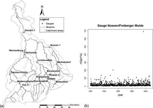
To compare the different approaches, we analysed flood series from 15 gauges in Germany, located in the Mulde River basin in Saxony (Fig. 3(a)) with an observation period of at least 75 years and floods recorded up to the year 2013. The catchment size varies between 75 and 5433 km². All data series contain several extraordinary extreme events. One of these events occurred in August 2002. Its exceptional value becomes evident in Fig. 3(b) (monthly discharge maxima at the Nossen gauge).

Figure 3. (a) Drainage basin of the River Mulde in Saxony and (b) monthly maximum discharges of the Nossen gauge from 1925 to 2013 on the River Freiberger Mulde.

We are aware that there could be some dependence in the time series when considering monthly maximum discharges. Nevertheless, we recognized in our calculations that the estimators used are, due to their robustness, able to cope with slight dependencies of monthly maxima. Additionally, the choice of a discharge threshold specifying monthly maxima as flood peaks reduces these dependencies to a negligible number. However, the influence of dependence needs to be studied further since the model is conceived for independent data, and an underlying process of dependence could lead to errors.

As a threshold to specify floods among the monthly maxima, we chose the minimum value of annual flood peaks of each series. For all gauges we compare POT and rPOT with the classical AMS concerning robustness and goodness of fit. For this purpose, we fit a GEV distribution to the AMS sample and the POT model to the whole sample using the PWM estimation and the TL-moments. For the GEV we concentrate on the more common estimator, the PWM.

To characterize the reliability or goodness of fit of the three different approaches, we used the criterion pval for all gauges. By application of the inverse distribution function, a quantile–quantile (QQ) plot can be used as a graphical tool to demonstrate the goodness of fit of pval for each fitting approach (Fig. 4). Often also a probability–probability plot is applied, but since a QQ-plot illustrates the extreme domains in a better way, we chose this presentation.

Figure 4. QQ plot of pval for (a) AMS, (b) POT and (c) robust POT approaches for gauges l = 1,…,15. When the estimation is reliable, the quantiles of pval equal those of the uniform distribution (thick black line).

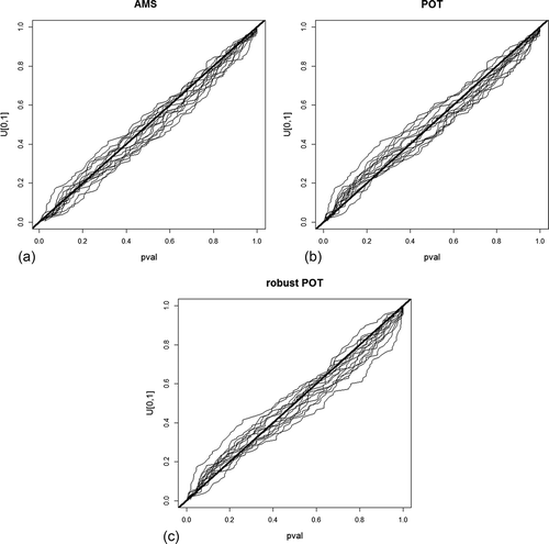
We can see that all three approaches give a good estimation of the distribution of the whole sample. In the area of the upper quantiles, POT seems to give the best goodness of fit, and all in all it does not differ much from the AMS statistic. For rPOT, a greater deviation exists for some gauges. Nevertheless, the deviation of all three approaches does not seem so large that we have to reject any of them. We are aware that the criterion pval could be affected by single extreme observations, which are most relevant for the fit of , but in the same way as for the evaluation of this fit. To consider this we also applied cross-validation, that is:

(15)

where is the fitted distribution function for gauge l based on all data except . The results we obtained from this approach were very similar to those of the original pval, so we can expect that the above mentioned problem did not influence our results.

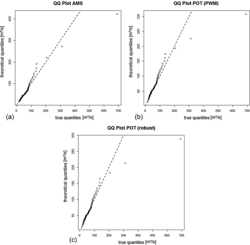
To investigate the fitting in the higher quantiles, where the difference in fitting seems to be largest, we look closely at the QQ-plot (Fig. 5) for the Nossen gauge (see above). Here it becomes evident how much the classical AMS model is influenced by the single extreme event, leading to a worse fitting to the higher quantiles. The POT model uses additional data values, which are mostly located in the lower domain. That is why it has a better fitting in the middle quantiles. Thus, the greater information spectrum leads to a more robust fitting. If the robustness is further increased by the application of the TL(0,1)-moment estimator, we can see a good fitting of all quantiles except the single extreme event.

Figure 5. QQ plots for the annual maximum discharges of the Nossen gauge and the estimates using (a) AMS (with PWM), (b) POT with PWM and (c) robust POT models. If the empirical quantiles of the gauge equal those of the model used, all data points can be found on the dotted line.

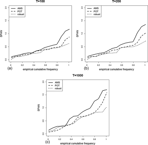
In the next step, the criterion SPAN_T was calculated for all 15 gauges for quantiles with annual return periods of 100, 200 and 1000 years. In Fig. 6 the empirical distributions of these vectors are plotted. The GEV approach with PWM estimators is most sensitive to changes in the data, having clearly higher SPAN_T scores for each of the three annual return periods. In general, the maximum value of SPAN_T increases with increasing T, indicating that the estimates become more sensitive for higher quantiles. This is understandable due to the small quantity of data in these high domains. The rPOT seems to be advantageous in the lower quantile areas, being much smaller than the other two approaches. In general, the main part of the calculated SPAN_T values for the robust POT approach were smaller, and therefore it is the most robust approach.

Figure 6. Empirical distribution of SPAN_T for annual return periods of (a) T = 100, (b) T = 200 and (c) T = 1000 years and all gauges. If the estimation is stable, the relative distance of the quantiles has to be close to zero and therefore also SPAN_T, consisting of the values of all single gauges, should be close to zero.

To have a closer look at these results, we analysed for one gauge (Nossen) values of SPAN_T that were derived from Monte Carlo simulations. We drew 1000 random samples of n = 50 years (for the POT approach this means 50 times 12 values per year) from the observed series. The 99.9% quantile, derived from the different models, was compared via SPAN_T with the quantile of the remaining 37 years of this series. The empirical distribution of SPAN_T can be found in Fig. 7. It becomes evident that the rPOT approach is the most robust, whereas the classical GEV model with PWM estimates is worst. We considered also the GEV model with maximum likelihood (ML) estimates, which is surprisingly more robust than the GEV–PWM model. Nevertheless, it resulted in the highest values of SPAN_T (≈ 2), indicating that for random samples where high flood peaks are concentrated in one subperiod, the estimated quantiles differ significantly from estimates from the other subsample. For samples in which the values within the two subperiods are similarly distributed, the high efficiency of the ML-estimator leads to small values of SPAN_T. In total, the robustness of the POT and rPOT approaches is less affected by the order of occurrence of the events in a data series.

Figure 7. Empirical distribution of SPAN₁₀₀₀ of Monte Carlo based random samples of the Nossen gauge for different models.

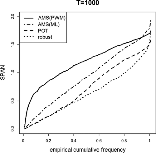
One remark: A comparison with the third classical estimation method, the method of moments, is not possible since the random samples can lead to a shape parameter , where the third moment and therefore the moment estimators no longer exist.

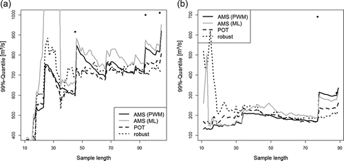
In the next step we analyse the robustness of quantiles of year-by-year increased time series for two gauges (Nossen and Wechselburg). We estimate the absolute deviation between the predicted return period and the observed return period (Tables 1 and 2). It becomes evident that after a certain time of stabilization, which is needed for an adequate modelling, the POT and especially the rPOT approach provide much more stable estimates of the annual return period than the classical annual maxima approach, AMS. Whereas the AMS approach is highly influenced by the occurrence of extreme events, the other two models are less responsive. At the Nossen gauge the flood in the year 2002 was so extreme that every model estimates return periods much higher than 25 000 years. A disadvantage of the rPOT models also becomes evident. In the year 2013 another extreme event occurred. Because of the very short time span since the previous extreme event in the year 2002, the non-robust AMS approach estimates a higher quantile, fitting well in this case. The rPOT handled the former extreme event as a type of outlier. When such an extreme event occurs a second time, however, some probability mass is given to this large flood. POT and rPOT now result in a larger difference. Comparing the evolving 99% quantiles from a series with an increasing length (Tables 3 and 4) with estimations, based on the total series, the deviations from the quantiles of the total series are smaller for the POT approaches. In most cases, the estimated return periods are reduced when the total series is used and are often close to the robust estimations. This shows the difficulties when estimating high quantiles from short data series with extreme events. When the series length increases, the estimation changes considerably.

Table 1. Absolute differences between predicted and observed return period of extraordinary extreme floods (Wechselburg/Zwickauer Mulde gauge, records beginning in the year 1910) with the three different fitting approaches. The return period of the observed flood was estimated with the time series ending in the years before the occurrence of this event. Only differences of more than 5 years are shown. The character ∞ stands for cases where the model was not able to fit a suitable distribution to the given data.

Series used for prediction	Year of the event	AMS	POT	rPOT
1910–1922	1923	3	34
1910–1923	1924	66	57 925
1910–1925	1926	10	68
1910–1931	1932	91	75	45
1910–1953	1954	354	444	88
1910–1974	1975	19	16	3
1910–2001	2002	172	124	38
1910–2012	2013	71	70	49

Table 2. The same content as in Table 1 but for the Nossen/Freiberger Mulde gauge (records beginning in the year 1926).

Series used for prediction	Year of observation	AMS	POT	rPOT
1926–1930	1931		30	1
1926–1953	1954	18	6	4
1926–1957	1958	750	65	29
1926–2001	2002	19 528 768	2 712 055	29 608
1926–2012	2013	31	127	353

Table 3. Flood peaks (in m³/s) with a return period of 100 years at the Wechselburg/Zwickauer Mulde gauge, derived from a series with a growing length and mean absolute deviation (MAD) from the results of the total series with four different approaches.

Series	AMS (ML)	AMS (PWM)	POT	rPOT
1910–1940	1516	687	690	824
1910–1950	649	613	619	728
1910–1960	814	792	717	716
1910–1970	755	714	684	702
1910–1980	829	766	725	729
1910–1990	753	713	717	733
1910–2000	757	720	709	726
1910–2010	822	800	754	726
1910–2013 (all)	953	919	791	708
MAD	231.9	193.4	89.1	34.5
MAD (%)	24.3	21	11.3	4.9

Table 4. Flood peaks (in m³/s) with a return period of 100 years at the Nossen/Freiberger Mulde gauge, derived from a series with a growing length and mean absolute deviation (MAD) from the results of the total series with four different approaches.

Series	AMS (ML)	AMS (PWM)	POT	robust POT
1926–1956	170	165	192	206
1926–1966	241	206	225	239
1926–1977	242	195	203	211
1926–1986	210	180	188	190
1926–1996	193	173	171	196
1926–2006	280	305	232	190
1926–2013 (all)	316	337	251	225
MAD	93.3	133	49.2	14.3
MAD (%)	29.5	39.5	19.6	7.4

The behaviour discussed above leads to the assumption that the rPOT results in an estimation of high quantiles that is stable over time and is less influenced by single extreme floods. Nevertheless, very extreme floods are still identified as extremely rare events. To demonstrate this, we compare the 99% quantiles of flood series with increasing sample lengths. As before, we started with the first 10 years of observations and estimated the 99% quantile from this sample. Then the sample length was increased step-by-step by 1 year and the 99% quantile was estimated. This was done up to the point where all recorded floods were included, in our case the year 2013. Plotting these results, the typical shape of the time series of quantiles is a “sawtooth” curve, as shown in Fig. 1. Every large event causes a jump in the quantile in the year of its occurrence. Afterwards, during periods with “normal” floods, these differences decrease slowly until the next large event occurs. Overall, we normally have a slight increase of the values of quantiles with growing sample length as more extreme events become more probable with the increase of the length of observations.

An example of such a moving quantile estimation is shown in Fig. 8 for the Wechselburg and Nossen gauges. For the classical AMS approach (GEV), we see the typical “sawtooth” curve, as mentioned above, regardless of the estimation method used (ML or PWM). Every large event leads to an abrupt increase of quantiles. This behaviour is, however, strongly damped when POT is used. Although there are still jumps in the estimated values, their magnitude is much smaller, and all in all we have a smaller variability of the quantiles and a smoother increase. For rPOT, when a robust parameter estimation with TL-moments is additionally used, we can see that the estimation is no longer affected by any jumps. However, at the beginning of the time series, the variability of quantiles estimated from the rPOT approach is high, an effect caused by the low efficiency of the TL(0,1) estimator for small samples, which is a typical characteristic of robust estimators.

Figure 8. Estimation of the 99% quantile (in m³/s) of the (a) Wechselburg and (b) Nossen gauges for growing sample length with three different approaches. The black dots are the annual maxima of single years.

One can also see that all three approaches need a sample length of at least 30 years to deliver stable results.

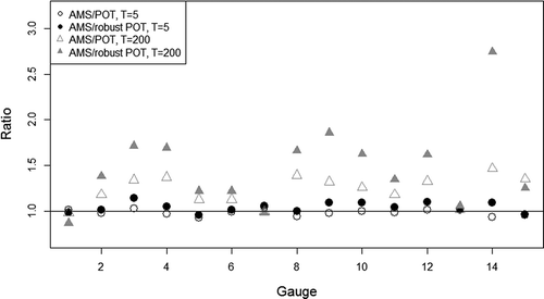
Additionally, we analysed the flood series for the other 13 gauges and calculated the coefficient of variation of the series of quantile estimations for the increasing sample lengths starting with 40 years (Fig. 9). As expected, the coefficient of variation for the POT is generally smaller than if we apply the classical AMS approach. The coefficient of variation for rPOT is a bit higher than the others. This results from the time needed for stabilization of the estimations. When a certain minimum length of the given series is ensured, the variation of results for rPOT decreases on average faster than that of the other approaches. Small quantiles are less affected by extremes than high quantiles. This is shown in Fig. 10 with the examples of the 80% and 99.5% quantiles of the whole samples. To compare the results, the ratios of the estimated floods between the AMS and both the POT and rPOT are used. One can see that the results of AMS estimations for a return period of T = 200 years are in general higher than the POT results (ratios greater than 1). Averaging all 15 gauges, this ratio is about 1.3. This means that, on average, the quantiles derived from AMS are 30% higher than using POT. Using rPOT, these differences become even higher. Here the flood quantiles are on average 50% smaller than those of AMS. The differences among quantiles with lower return periods, e.g. T = 5, are much smaller, regardless of the estimation approach. So, rPOT only affects the higher quantiles by giving less weight to the influence of extreme events. This supports the results concerning the reliability of POT or rPOT.

Figure 9. Coefficient of variation of the 99% quantile estimation for increasing sample length with three different approaches for 15 gauges of the Mulde basin.

Figure 10. Comparison of the AMS and the POT (white) and the robust POT (filled) by the ratio between the flood quantiles 0.8 and 0.995.

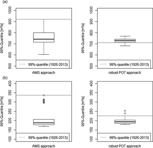
As was shown in Figs 1 and 8, flood quantiles change with the length of the flood series and the occurrence of extreme floods. The rPOT approach (after a certain period needed for its stabilization) results in a low variability of extreme quantiles. Compared to the AMS-estimated quantiles derived from the total series of observations, these “final” quantiles are much smaller, since the extreme flood in the year 2013 has less impact (Fig. 10). However, the rPOT quantiles for the series up to the year 2013 are similar to the estimated quantiles of all shorter recorded series (Fig. 8). This is not the case for the AMS approach. To show the differences in the results between the two approaches, we calculated the frequencies of the 99% flood quantiles for year-by-year increasing series of observations starting with a series of at least 40 years of observation and ending in the year 2013 (Fig. 11). The results are shown in box plots of both methods for two gauges. The flood range where the highest frequencies are concentrated is quite similar for both methodologies, but rPOT avoids very high estimations of these quantiles. For rPOT, all estimated quantiles are grouped close together, having small deviations. The quantile for the total series up to 2013 is located close to the centre of the boxplot, that is, the median of all estimated quantiles. In contrast, the range of the box plot for AMS-based quantiles is broader, and the quantile of the total series is located far from the centre of the boxplot. For the Nossen gauge it is even in the range of outliers. Comparing the mean and median of the estimated quantiles, they do not differ much for both approaches (about 5–10%), therefore one can say that over time both approaches in general come to the same results, although the rPOT leads to less variation.

Figure 11. Boxplots of all estimated 99% quantiles derived from the AMS or the robust POT approaches for year-by-year increasing sample lengths starting with a length of 40 for the (a) Wechselburg and (b) Nossen gauges. The estimated 99% quantiles for the full recorded series for AMS and robust POT (grey line) are also shown.

5 Conclusions

The distribution of flood quantiles by partial duration series is a combination of two distributions, one for the annual number of exceedences and the other for the magnitude of exceedences. Although the Poisson distribution does not seem to fit in a large number of cases, replacement by other, better fitting distributions does not make a difference in the estimation of annual return periods and can therefore be omitted.

In comparison with the classical AMS approach, POT and rPOT are robust alternatives, which have advantages particularly in the estimation of high flood quantiles for series with rare but very extreme events. They deliver a stable estimation of high quantiles over large time periods and avoid sudden jumps in flood estimations. Therefore, they give stability in the estimation, which satisfies our criteria for robustness. However, for all 15 gauges of our analysis, we needed a sample length of at least 30 years to get stable results for the rPOT approach (see Fig. 8). We detect the same behaviour if we start with the end of the series and extend it step by step to the first observation. Thus, the robust POT approach should be used only for samples with a length of at least 30 years, otherwise the efficiency of the estimator will be too low. In the presence of extreme events, the estimation based on POT or rPOT is generally lower than that based on the classical AMS approach. Therefore, the acceptance of the resulting changes in flood quantiles can be critical for many estimations. However, additional benefits of rPOT can be expected for the regionalization of flood quantiles, where it compensates up to a certain degree for the impact of different time lengths in a region.

Additional information

Funding

The financial support of the Deutsche Forschungsgemeinschaft (SFB 823, “Statistical modelling of nonlinear dynamic processes”) is gratefully acknowledged.

APPENDIX: TL-moments

Trimmed linear-moments (TL-moments) are a robust modification of L-moments developed by Hosking (1990). They were introduced by Elamir and Seheult (2003) and, due to their easy computation, are frequently used and developed for many different distributions (cf. Hosking 2007, Abdul-Moniem and Selim 2009, Ahmad et al. 2011). Let X be a real-valued random variable with cumulative distribution function F. The rth TL-moment with trimming (t₁,t₂) is given by:

(A1)

where we can use the representation:

(A2)

of the expected value of the ith-order statistic of a sample with length r drawn from the distribution of X. x(F) is the quantile function of the distribution of X, in our case the GPD with:

(A3)

In this paper the location parameter u is known since we choose a threshold .

An unbiased estimate of is:

(A4)

The main idea of this kind of estimator to gain robustness is censoring by giving zero weight to the t₁ smallest and t₂ largest values. In our case we want to have robustness against single large events for an estimator of the parameter of the GPD. The lower part of the sample is already censored by choosing a threshold and only considering values above this threshold (see Section 2). Therefore, we chose t₁ = 0 and t₂ = 1. For the cases t₁ = t₂ = 1 and t₁ = 1, t₂ = 0, estimators for the GPD are already developed (Abdul-Moniem and Selim 2009, Ahmad et al. 2011), and Hosking (2007) developed TL(0,1) estimators for the two-parameter GPD. We want to consider the three-parameter GPD as well, which is why we present the explanation in the calculations below.

Explicit representations of the first three TL(0,1)-moments are:

(A5)

We can see that indeed the highest value of the order statistics is left out in the calculation.

With the equations above, the first three TL(0,1)-moments can be written as:

(A6)

and the ratio:

(A7)

By calculating the integrals above and using substitution, we obtain the following estimators, where the TL(0,1)-moments are estimated via (A4):

(A8)

If is known, we get (analogous to Hosking 2007):

(A9)

Since the choice of the trimming factors is crucial, especially in our context with several extreme values, it is necessary to consider not only TL(0,1)-moments but also other choices for the trimming factors. As mentioned above, a trimming in the lower part of the sample is not meaningful. However, we consider a higher trimming in the upper part of the sample, that is, the TL(0,2)-moments.

Analogously to the TL(0,1)-moments we can calculate:

(A10)

and

(A11)

Or, if is known:

(A12)

References

- Abdul-Moniem, I. and Selim, Y.M., 2009. TL-moments and L-moments estimation for the generalized Pareto distribution. Applied Mathematical Sciences, 3 (1), 43–52.
- Ahmad, U.N., Shabri, A., and Zakaria, Z.A., 2011. Trimmed L-moments (1,0) for the generalized Pareto distribution. Hydrological Sciences Journal, 56 (6), 1053–1060. doi:10.1080/02626667.2011.595719
- Asquith, W.H., 2007. L-moments and TL-moments of the generalized lambda distribution. Computational Statistics & Data Analysis, 51 (9), 4484–4496. doi:10.1016/j.csda.2006.07.016
- Balkema, A.A. and Haan, L. de., 1974. Residual life time at great age. The Annals of Probability, 2 (5), 792–804. doi:10.1214/aop/1176996548
- Bárdossy, A. and Singh, S.K., 2008. Robust estimation of hydrological model parameters. Hydrology and Earth System Sciences Discussions, 5 (3), 1641–1675. doi:10.5194/hessd-5-1641-2008
- Beguería, S., 2005. Uncertainties in partial duration series modelling of extremes related to the choice of the threshold value. Journal of Hydrology, 303 (1–4), 215–230. doi:10.1016/j.jhydrol.2004.07.015
- Brigode, P., Oudin, L., and Perrin, C., 2013. Hydrological model parameter instability: a source of additional uncertainty in estimating the hydrological impacts of climate change? Journal of Hydrology, 476 (0), 410–425. doi:10.1016/j.jhydrol.2012.11.012
- Cunnane, C., 1973. A particular comparison of annual maxima and partial duration series methods of flood frequency prediction. Journal of Hydrology, 18 (3–4), 257–271. doi:10.1016/0022-1694(73)90051-6
- Cunnane, C., 1979. A note on the Poisson assumption in partial duration series models. Water Resources Research, 15 (2), 489–494. doi:10.1029/WR015i002p00489
- Elamir, E.A.H. and Seheult, A.H., 2003. Trimmed L-moments. Computational Statistics and Data Analysis, 43 (3), 299–314. doi:10.1016/S0167-9473(02)00250-5
- Fisher, R.A. and Tippett, L.H.C., 1928. Limiting forms of the frequency distribution of the largest or smallest member of a sample. Mathematical Proceedings of the Cambridge Philosophical Society, 24 (02), 180–190.
- Garavaglia, F., et al., 2011. Reliability and robustness of rainfall compound distribution model based on weather pattern sub-sampling. Hydrology and Earth System Sciences, 15 (2), 519–532. doi:10.5194/hess-15-519-2011
- Greenwood, J.A., et al., 1979. Probability weighted moments: definition and relation to parameters of several distributions expressable in inverse form. Water Resources Research, 15 (5), 1049–1054. doi:10.1029/WR015i005p01049
- Grubbs, F.E., 1969. Procedures for detecting outlying observations in samples. Technometrics, 11 (1), 1–21. doi:10.1080/00401706.1969.10490657
- Guerrero, J.-L., et al., 2013. Exploring the hydrological robustness of model-parameter values with alpha shapes. Water Resources Research, 49 (10), 6700–6715. doi:10.1002/wrcr.20533
- Gumbel, E.J. and Schelling, H. von, 1950. The distribution of the number of exceedances. Annals of the Mathematical Statistics, 21 (2), 247–262. doi:10.1214/aoms/1177729842
- Hosking, J.R.M., 1990. L-moments: analysis and estimation of distributions using linear combinations of order statistics. Journal of the Royal Statistical Society. Series B (Methodological), 52 (1), 105–124.
- Hosking, J.R.M., 2007. Some theory and practical uses of trimmed L-moments. Journal of Statistical Planning and Inference, 137 (9), 3024–3039. doi:10.1016/j.jspi.2006.12.002
- Hosking, J.R.M., Wallis, J.R., and Wood, E.F., 1985. Estimation of the generalized extreme-value distribution by the method of probability-weighted moments. Technometrics, 27 (3), 251–261. doi:10.1080/00401706.1985.10488049
- Huber, P.J., 2004. Robust statistics. New York: Wiley.
- Klemeš, V., 1986. Dilettantism in hydrology: transition or destiny? Water Resources Research, 22 (9S), 177S–188S. doi:10.1029/WR022i09Sp0177S
- Kochanek, K., et al., 2013. A data-based comparison of flood frequency analysis methods used in France. Natural Hazards and Earth System Sciences Discussions, 1 (5), 4445–4479. doi:10.5194/nhessd-1-4445-2013
- Kumar, P., Guttarp, P., and Foufoula-Georgiou, E., 1994. A probability-weighted moment test to assess simple scaling. Stochastic Hydrology and Hydraulics, 8 (3), 173–183. doi:10.1007/BF01587233
- Langbein, W.B., 1949. Annual floods and the partial-duration flood series. Transactions of the American Geophysical Union, 30 (6), 879.
- Madsen, H., Rasmussen, P.F., and Rosbjerg, D., 1997. Comparison of annual maximum series and partial duration series methods for modeling extreme hydrologic events: 1. At-site modeling. Water Resources Research, 33 (4), 747–757. doi:10.1029/96WR03848
- Malamud, B.D. and Turcotte, D.L., 2006. The applicability of power-law frequency statistics to floods. Journal of Hydrology (Special Issue: International Conference “Hydrofractals '03”) 322 (1–4), 168–180. doi:10.1016/j.jhydrol.2005.02.032
- (Natural Environment Research Council), ed., 1975. Flood studies report (five volumes). London: Natural Environment Research Council. Available online at: http://nora.nerc.ac.uk/5964/1/IH_094.pdf
- Önöz, B. and Bayazit, M., 2001. Effect of the occurrence process of the peaks over threshold on the flood estimates. Journal of Hydrology, 244 (1–2), 86–96. doi:10.1016/S0022-1694(01)00330-4
- Ouarda, T.B. and Ashkar, F., 1998. Effect of trimming on LP III flood quantile estimates. Journal of Hydrologic Engineering, 3 (1), 33–42. doi:10.1061/(ASCE)1084-0699(1998)3:1(33)
- Pickands III, J., 1975. Statistical inference using extreme order statistics. The Annals of Statistics, 3 (1), 119–131. doi:10.1214/aos/1176343003
- Rasmussen, P.F. and Rosbjerg, D., 1991. Prediction uncertainty in seasonal partial duration series. Water Resources Research, 27 (11), 2875–2883. doi:10.1029/91WR01731
- Renard, B., et al., 2013. Data-based comparison of frequency analysis methods: A general framework. Water Resources Research, 49 (2), 825–843. doi:10.1002/wrcr.20087
- Rosbjerg, D., 1985. Estimation in partial duration series with independent and dependent peak values. Journal of Hydrology, 76 (1–2), 183–195. doi:10.1016/0022-1694(85)90098-8
- Rosbjerg, D., Madsen, H., and Rasmussen, P.F., 1992. Prediction in partial duration series with generalized pareto-distributed exceedances. Water Resources Research, 28 (11), 3001–3010. doi:10.1029/92WR01750
- Rosner, B., 1983. Percentage points for a generalized ESD many-outlier procedure. Technometrics, 25 (2), 165–172. doi:10.1080/00401706.1983.10487848
- Salinas, J.L., et al., 2014. Regional parent flood frequency distributions in Europe – Part 1: Is the GEV model suitable as a pan-European parent? Hydrology and Earth System Sciences, 18 (11), 4381–4389. doi:10.5194/hess-18-4381-2014
- Shane, R.M. and Lynn, W.R., 1964. Mathematical model for flood risk evaluation. Journal of the Hydraulics Division, 90 (6), 1–20.
- Spencer, C.S. and McCuen, R.H., 1996. Detection of outliers in Pearson type III data. Journal of Hydrologic Engineering, 1 (1), 2–10. doi:10.1061/(ASCE)1084-0699(1996)1:1(2)
- Stedinger, J.R., Vogel, R.M., and Foufoula-Georgiou, E., 1993. Frequency analysis of extreme events. In: D.R. Maidment, ed. Handbook of hydrology. Chapter 18. New York: McGraw-Hill, 66p.
- Taesombut, V. and Yevjevich, V., 1978. Use of partial series for estimating the distribution of maximum annual flood peak. Hydrology Paper, 97, Colorado State University, Fort Collins, Colorado.
- Tavares, L.V. and Da Silva, J.E., 1983. Partial duration series method revisited. Journal of Hydrology, 64 (1–4), 1–14. doi:10.1016/0022-1694(83)90056-2
- Wang, Q.J., 1997. LH moments for statistical analysis of extreme events. Water Resources Research, 33 (12), 2841–2848. doi:10.1029/97WR02134