Improvement of artificial neural networks to predict daily streamflow in a semi-arid area

ABSTRACT

The application of artificial neural networks (ANNs) has been widely used recently in streamflow forecasting because of their flexible mathematical structure. However, several researchers have indicated that using ANNs in streamflow forecasting often produces a timing lag between observed and simulated time series. In addition, ANNs under- or overestimate a number of peak flows. In this paper, we proposed three data-processing techniques to improve ANN prediction and deal with its weaknesses. The Wilson-Hilferty transformation (WH) and two methods of baseflow separation (one parameter digital filter, OPDF, and recursive digital filter, RDF) were coupled with ANNs to build three hybrid models: ANN-WH, ANN-OPDF and ANN-RDF. The network behaviour was quantitatively evaluated by examining the differences between model output and observed variables. The results show that even following the guidelines of the Wilson-Hilferty transformation, which significantly reduces the effect of local variations, it was found that the ANN-WH model has shown no significant improvement of peak flow estimation or of timing error. However, combining baseflow with streamflow and rainfall provides important information to ANN models concerning the flow process operating in the aquifer and the watershed systems. The model produced excellent performance in terms of various statistical indices where timing error was totally eradicated and peak flow estimation significantly improved.

Editor D. Koutsoyiannis; Associate editor Y. Gyasi-Agyei

KEYWORDS:

• artificial neural networks
• daily streamflow prediction
• peak flow estimation
• timing error
• Wilson-Hilferty transformation
• baseflow separation

1 Introduction

The transformation relating streamflow to rainfall is highly complex and nonlinear because it is influenced by numerous factors, including the temporal and spatial distribution of rainfall, land use, topography and soil characteristics. This complex nonlinear process is not easily described by a simple model, which makes accurate forecasting very difficult.

Numerous streamflow forecasting techniques have been suggested and used in the past. They generally fall under statistical/stochastically based and conceptual/physically based techniques (Salas et al. 2000). However, these models are very data/time demanding and require a large number of parameters, which are not always available, especially in semi-arid areas.

One of the powerful tools that are able to capture the complex dynamics of a watershed without requiring a lot of hydrological data is artificial neural networks (ANNs). An ANN is not programmed like a conventional computer program, but is presented with examples of the patterns, observations and concepts, or any type of data it is supposed to learn. Through the process of learning, the neural network organizes itself to develop an internal set of features that it uses to classify information or data. This technique is based on extracting and also re-using information that is implicitly contained in hydrological data without directly taking into account the physical laws that underlie the rainfall–runoff processes (De Vos and Rientjes 2005).

The application of ANNs to forecast problems in hydrology has been one of the major goals for hydrologists. There has been a rapidly growing interest among water scientists to apply neural networks in water resources. Indeed, ANNs have been applied in forecasting long-term rainfall (Karamouz et al. 2008, Mekanik et al. 2013), forecasting sea level (Pashova and Popova 2011), forecasting floods (Tiwari and Chatterjee 2010), forecasting water quality (Robert et al. 2008, Banerjee et al. 2011), forecasting daily water demands (Bennett et al. 2013), flow forecasting (Huo et al. 2012, Kalteh 2013, Mohanty et al. 2013), snowmelt–runoff forecasting (Yilmaz et al. 2011), modelling rainfall–runoff processes (Tsung-yi and Wang 2004, Kisi 2008, Wu and Chau 2011), rainfall forecasting (Wu et al. 2010), sediment transport prediction (Hamidi and Kayaalp 2008, Melesse et al. 2011, Kisi et al. 2012, Lafdani et al. 2013), groundwater level forecasting (Krishna et al. 2008, Nourani et al. 2008) and determination of aquifer parameters (Samani et al. 2007, Lin et al. 2010).

Despite the success of ANNs in many fields and the strong theoretical background, many hydrologists indicate that ANNs are unable to well simulate peak flow values in streamflow time series (e.g., Campolo et al. 1999, Sudheer et al. 2003). In addition, it was found that ANN simulation is affected by time lagging between simulated and observed streamflow series (e.g., Minns 1998, De Vos and Rientjes 2005). Sudheer et al. (2003) attributed the underestimation of peak flow values to the local variations in the function being mapped. On the other hand, lagging prediction was attributed to the high autocorrelation of the flow data (Jain and Srinivasulu 2004, De Vos and Rientjes 2005). According to Wu et al. (2009), these problems can be viewed as a consequence of various noises that affect the flow signal at different levels. Sudheer et al. (2003) suggested that an appropriate data transformation based on a statistical model can improve the peak flow estimation. As for reducing the effect of time lagging, De Vos and Rientjes (2005) proposed the use of a moving average (MA) over flow data to obtain new data inputs. As is known, streamflow and rainfall data in arid and semi-arid areas are affected by many local variations due to the varying skewness in the data. In addition, flow series can be viewed as a sum of multiple signals, especially quickflow and baseflow. Adequate hydrological signals used as model inputs will improve the model performance.

In this paper we deal with the problems of peak flow prediction and time lagging in ANN-based river flow modelling. To improve the peak flow simulation by ANNs and minimize the effect of time lagging, two approaches were used and coupled with ANNs to build three ANN models. The first approach is based on the pre-processing technique of the Wilson-Hilferty stochastic model (Wilson and Hilferty 1931), which was coupled with an ANN (ANN-WH). The second approach is based on incorporating hydrological knowledge into the modelling process through the use of baseflow components. Two different baseflow separation techniques were used and coupled with ANNs: the recursive digital filter (ANN-RDF) and the one parameter digital filter (ANN-OPDF).

The three models (ANN-WH, ANN-RDF and ANN-OPDF) were used to improve ANN performance by removing the time lag between predicted and observed streamflow by reducing the high autocorrelation function of flow, which causes the introduction of the autoregressive component in the ANN, and increasing the network performance to simulate peak flows.

2 Artificial neural networks

The network used in the current study is the multilayer feedforward neural network (MFNN). This type of ANN is the most commonly used architecture for streamflow forecasting (Gupta et al. 2000). Its popularity stems mainly from the theoretical ability of the MFNN to approximate complicated nonlinear (differentiable and bounded) functions to arbitrary accuracy (Funahashi 1989, Hornik et al. 1989, Hornik 1991). The true computing power of the ANN comes through connecting multiple neurons, though even a single neuron can perform a substantial level of computation (Lerma and Leonardo 1992). To achieve a higher level of computational capabilities, a more complex structure of ANN is required. In a multilayer structure, the input nodes pass the information to the units in the first hidden layer, and then the outputs from the first hidden layer are passed to the next layer, and so on. A multilayer network can also be viewed as cascading of groups of single-layer networks. The level of complexity in computing can be seen by the fact that many single-layer networks are combined into this multilayer network. The design of an ANN should consider how many hidden layers are required, depending on the complexity of the desired computation (Kawaguchi 2000).

3 Study area and data

The area considered in the current study is the Anseghmir River basin (Fig. 1); it belongs to the upper Moulouya watershed. The basin area is 967 km², representing about 20% of the total surface of the upper Moulouya. The maximum elevation is ~3713 m and the minimum is 1313 m. The climate is arid to sub-arid, receiving an average rainfall of 188 mm/year. The region is characterized by a severe winter and a hot summer, influenced by seasonal temperature variations, although summer is characterized by heavy showers, which make the area prone to flooding (Zemzami et al. 2013). These rains are not directly involved in river flow, but are stored in different reservoirs (mainly in hillslopes) for very long periods (many days) before being released in a few minutes, which explains the dominance of old water compared to new water in the river, and also the low rainfall–runoff correlation compared to the streamflow correlation. Thus, the flood hydrograph is dominated by old water (pre-event water) (Sklash et al. 1976, Genereux and Hooper 1998).

Figure 1. Location of the study watershed.

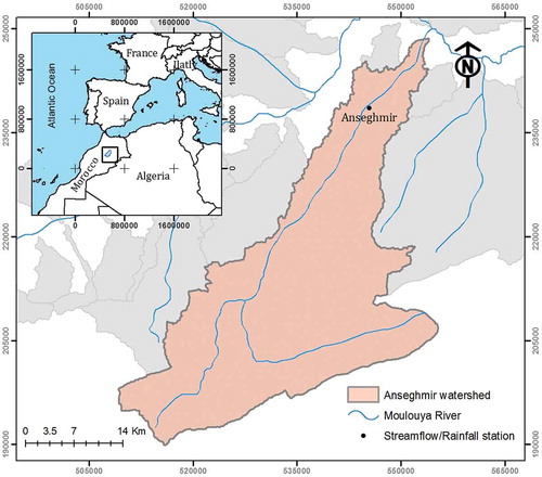
The study site has daily streamflow and rainfall data. The streamflow gauge station (Anseghmir) is located in the downstream section of the river while the rain gauge station is located in the upstream section.

Twenty consecutive water years of the daily rainfall and streamflow dataset (1990 to 2009) for the Anseghmir River basin were used. The first 12 years were used to train the network; the next 4 years are used to validate how well the network generalized. Finally, the last 4 years provided an independent test of network generalization to data that the network has never seen.

4 Methods

4.1 Model evaluation

The evaluation of ANN performance in hydrology is achieved by several methods and criteria. This evaluation aims to determine performance of the model for different situations. The literature presents a wide variety of assessment methods. In the current paper, we used three measures to evaluate the model response:

The root mean squared error, RMSE:

the Nash-Sutcliffe coefficient, C_NS (Nash and Sutcliffe 1970):

and the persistence index, C_IP (Kitanidis and Bras 1980):

where is observed streamflow, simulated streamflow, average streamflow and n the number of data elements.

These measures provide useful insights into the behaviour of the model in different situations. RMSE is used for peak flow evaluation and complete assessment of the model error, C_NS for overall performance and goodness of fit, and C_IP is used to check the prediction lag effect.

4.2 Wilson-Hilferty model

It is known that streamflow time series (or other hydrological time series) can be presented by deterministic and stochastic components. Appropriate techniques for removing and modelling series with trends and jumps can improve the performance of a hydrological model (Marco et al. 1993). Moving average, data normalization or statistical modelling can be used to reduce the effect of these components. However, the accuracy of these methods has shown small or no improvement of ANNs (De Vos 2003). Sudheer et al. (2003) proposed reducing the effect of local variation in the function being mapped by the use of the Wilson-Hilferty transformation (WH) in ANN modelling to improve model performance. Theoretically, if the guidelines to Wilson-Hilferty model building are followed in the ANN approach, the performance of an ANN may be improved significantly (Sudheer et al. 2003). The use of the Wilson-Hilferty transformation implies an approximation to a chi-square variable and is theoretically limited to small values of the skewness coefficient (γ < 2). For values up to 9.0, Kirby (1972) suggested a modification of the Wilson-Hilferty transformation. The raw data Q are first log-transformed:

(1)

Q_J is the flow for day J, Y is the year.

Standardization is obtained by:

(2)

The modified Wilson-Hilferty transformation according to Kirby (1972) is expressed by:

(3)

where S′_Y,_J satisfies the conditions:

(4)

where γ_J is the skewness coefficient of the raw data.

The modified Wilson-Hilferty transformation is valid for any value of skewness coefficient that preserves the first three moments.

4.3 Baseflow separation methods

Baseflow (BF) separations have been widely studied and have a long history in hydrological sciences (Hall 1968, Tallaksen 1995). They are used to extract the two major components of a hydrograph: baseflow (groundwater discharge into a stream) and quickflow (surface runoff). Numerous non-tracer-based and tracer-based separation methods have been developed to separate baseflow from total flow. In the first group, we found digital filters that are originally in the signal processing. Digital filtering removes a large part of the errors due to the subjectivity of manual separation, thereby providing consistent and reproducible results. Many types of filters are reported in the literature. Thus, we chose two types of filters that minimize the subjective influence of the user for hydrograph separation: the one parameter digital filter, OPDF (Lyne and Hollick 1979, Nathan and McMahon 1990, Arnold and Allen 1999), and the recursive digital filter, RDF (Eckhardt 2005). Equation (5) shows the OPDF, while equation (6) shows RDF:

(5)

(6)

where q_k and q_k−1 are, respectively, direct runoff at time k and time k − 1, y_k and y_k−1 are respectively total streamflow at time k and k − 1, a is a filter parameter, b_k and b_k−1 are, respectively, baseflow at time steps k and k − 1, and BFI_max is maximum baseflow index.

5 Application

5.1 Wilson-Hilferty model application

The time series used as inputs to forecast daily streamflow are clearly asymmetric with the existence of several local variations (Fig. 2). The skewness of streamflow and rainfall data are, respectively, 6.51 and 8.75, which confirms the existence of local variations in the two functions. According to Sudheer et al. (2003), to provide an accurate estimate of the peak flows using ANN, it is necessary to remove the local variations caused by these high values of rainfall and streamflow from the time series function being mapped.

Figure 2. Raw and transformed rainfall–streamflow time series using the Wilson-Hilferty model.

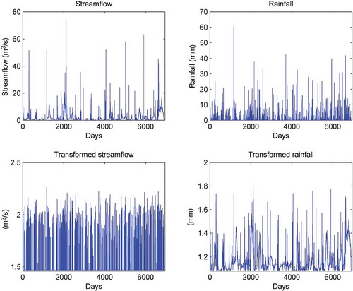
Figure 2 displays transformed times series using the Wilson-Hilferty model. The application of the Wilson-Hilferty transformation showed a significant reduction of the local variation effect in streamflow and rainfall time series. Skewness coefficient and standard deviation of streamflow and rainfall were significantly reduced. The statistical description of raw and transformed data is represented in Table 1.

Table 1. Statistics of raw and transformed data using the Wilson-Hilferty model.

	Raw data		Transformed data
	Rainfall	Streamflow	Rainfall	Streamflow
Minimum	0.01	0.001	1.47	1.09
Maximum	60.40	74.5	2.26	1.80
Mean	0.57	1.83	1.52	1.16
Standard deviation	2.56	3.66	0.15	0.10
Skewness	8.75	6.51	2.71	2.18

It is noted that the effectiveness of removing local variations using the Wilson-Hilferty transformation depends on the statistical properties of time series. Indeed, the transformed streamflow data are a smoother function than the transformed rainfall data.

5.2 Baseflow separation application

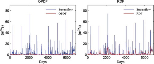
The baseflow component of the Anseghmir streamflow time series was separated using the OPDF and RDF. The RDF and OPDF need the determination of the recession constant a. In addition, the RDF requires that the maximum value of the baseflow index (BFI_max), which indicates the long-term ratio of baseflow to total streamflow, should be determined.

The higher the BFI_max value is, the higher the baseflow component, and vice versa. This value is determined numerically and may be calibrated. The knowledge of BFI_max requires a large amount of information on surface runoff and subsurface flow in the watershed. To minimize the subjective influence of the choice of BFI_max, it is necessary to find typical values that are related to watershed characteristics. Studies carried out by the Hydraulic Basin Agency of Moulouya (ABHM 2008) showed the existence of a hard rock aquifer consisting of Dogger limestone and dolomite. Based on the ABHM reports and analysis of hydrological and hydrogeological characteristics of the Anseghmir watershed, the value of 0.27 is suggested for BFI_max. Similarly, the recession parameter was 0.925 for the OPDF and 0.719 for the RDF. Figure 3 illustrates the component of baseflow to total streamflow for both the OPDF and RDF.

Figure 3. Baseflow separation using RDF and OPDF.

5.3 ANN architecture

The network architecture concerns the number of hidden neurons and the determination of relevant inputs. Based on the trial and error approach, the optimal number of neurons in the hidden layer was found to be 20 neurons.

The selection of model inputs is difficult in ANN development. Bowden et al. (2005) have reviewed and reported a large number of methods that can be used for ANN input selection. However, there is no theoretical guide for the selection of model inputs because these methods appear very subjective, and thus the trial and error approach is justified (Wu et al. 2009). A good alternative to the trial and error approach was proposed by Sudheer et al. (2002), suggesting that the statistical approach depending on cross-, auto- and partial auto-correlation of the observed data is a good method in identifying model inputs. These methods have been successfully used by many researchers (Kisi 2008, Wu et al. 2009).

To determine the candidate ANN inputs we used (1) a cross-correlation function (CCF) and a partial auto-correlation function (PACF) at various lags to determine the strength of the input–output relationship (Fig. 4), and (2) stepwise selection, which is aimed at handling redundancy of information between candidate variables. The proposed methods were used for searching through the many possible combinations of inputs and determining a near optimal set, while working within high input dimensions. Finally, the appropriate model inputs are determined using the trial and error approach based on the results of the previous approaches.

Figure 4. Plot of the PACF and CCF for (a) streamflow, (b) rainfall, (c) WH streamflow, (d) WH rainfall, (e) OPDF baseflow and (f) RDF baseflow, where the red lines stand for the 95% confidence bound.

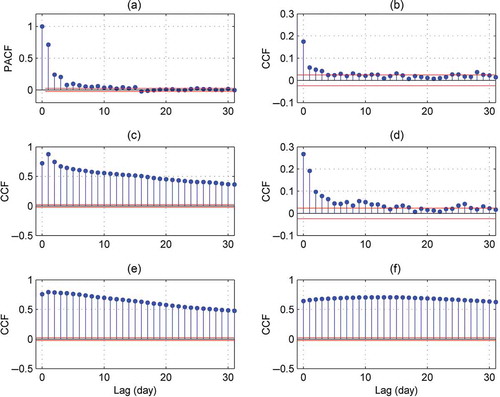
Table 2 shows the principal results obtained using the CCF, PACF and stepwise elimination approaches. For suitable ANN inputs, the two methods proposed different combinations. However, due to the high correlation for the first 30 lags between streamflow and pre-processed rainfall using the WH model, OPDF and RDF, it was found that the CCF was unable to determine a suitable time lag for ANN inputs.

Table 2. ANN input selection using PACF, CCF and stepwise approaches.

Input variable	Time lag (i)
	CCF and PACF	Stepwise
Q(t − i)	1, 2, …,7, 8	0, 1, 2, 4, 5, 8, 10, 12, 14
R(t − i)	0, 1, 2, 3	1, 2, …, 29, 30
WHQ(t − i)	Not identifiable	0, 1, 2, 3, 6, 10, 30
WHR(t − i)	1, 2, …, 11, 12	1, 2, …, 28, 29 (except 14)
OPDF(t − i)	Not identifiable	0, 1, 4, 6, 8, 14
RDF(t − i)	Not identifiable	0, 1, 2, 5, 14, 23

Based on the results obtained in Table 2 and the use of the trial and error approach, the final selection of model inputs were:

Table

ANN:	Q(t, t − 1, t − 2, t − 3)
	R(t, t − 1, t − 2, t − 3, t − 4, t − 5, t − 6)
ANN-WH:	WHQ(t, t − 1, t − 2, t − 3, t − 4)
	WHR(t, t − 1, t − 2, t − 3, t − 4, t − 5, t − 6)
ANN-OPDF:	Q(t, t − 1, t − 2, t − 3, t − 4)
	R(t, t − 1, t − 2, t − 3, t − 4)
	BF(t, t − 1, t − 2, t − 3, t − 4, t − 5, t − 6)
ANN-RDF:	Q(t, t − 1, t − 2, t − 3, t − 4)
	R(t, t − 1, t − 2, t − 3, t − 4)
	BF(t, t − 1, t − 2, t − 3, t − 4, t − 5, t − 6)

The number of hidden neurons in the hidden layer was effectively the same for the four models. The best results were obtained using 16 neurons.

6 Results and discussion

The ANN model was used as a reference to compare the effectiveness of the proposed methods. The network inputs consisted of previously raw values of rainfall and streamflow data. The obtained C_NS and C_PI coefficients are, respectively, 0.66 and 0.42, which indicate that the forecasted performance of the ANN at the Anseghmir watershed has had difficulties in making a good prediction. Figure 5(a) shows details of the simulated hydrograph in which the main drawbacks of the ANN prediction were the under- and overestimation of peak flow values and the time lag between observed and simulated streamflow. This indicates that the ANN model produces a poor prediction and was unable to make the correct timing between observed and forecasted streamflow time series. The low values of C_NS and C_PI demonstrate this fact. The scatter plot of the results obtained is illustrated in Fig. 6(a). The point clouds are clearly scattered and show poor correlation. Based on extensive tests, it was found that the effect of time lag is always present and is closely linked to the use of previous values of streamflow, which introduce an autoregressive component in the model and thus generate a timing error in the model prediction. The maximum value of the CCF is shifted on the left of the zero lag axis and found to be −1 day, which indicates that the simulation is affected by the timing lag (Fig. 7(a)).

Figure 5. Detail of observed and forecasted streamflow using (a) ANN, (b) ANN-WH, (c) ANN-OPDF and (d) ANN-RDF.

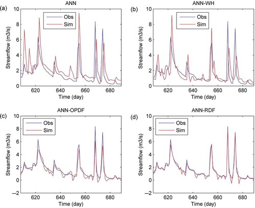
Figure 6. Scatter plot of observed and forecasted streamflow using (a) ANN, (b) ANN-WH, (c) ANN-OPDF and (d) ANN-RDF.

Figure 7. Cross-correlation function between observed and forecasted streamflow using (a) ANN, (b) ANN-WH, (c) ANN-OPDF and (d) ANN-RDF.

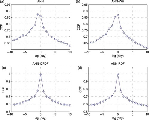
Concerning the Wilson-Hilferty transformation, three models were developed to forecast daily streamflow. The first model consists of transformed inputs (streamflow and rainfall). The second model was fed by transformed streamflow data and raw rainfall data. Finally, the third model uses raw streamflow and transformed rainfall. The best results were obtained using the second model. As can be evidenced by the decrease of RMSE compared with the ANN model, the ANN-WH was relatively able to increase accuracy of peak flow estimation and overall performance. Although the model efficiency was improved over the ANN model, the prediction accuracy is still unsatisfactory. The C_NS and C_PI statistics, which are respectively 0.69 and 0.46, indicate that the model is always unable to overcome the problems of lag time and peak flow estimation. The prediction time lag is fairly obvious and the model prediction does not reproduce low flows and recession curves reasonably well (Fig. 5(b)). Figure 5(b) shows a simulated hydrograph in which the forecasted streamflow is far from a good simulation. The effectiveness of data transformation is not evident and many peaks are not well mapped by the ANN-WH. It can also be seen from the scatter plot of Fig. 7(b) that there was no significant change in the network performance compared to ANN model. In Fig. 6(b), the maximum value of the CCF was obtained at time lag 0 day and reached 0.86. The second high autocorrelation value was obtained at time lag −1 day and reached 0.85. This fact shows that the time lag between predicted and observed time series was reduced compared to that of the ANN model, but not removed.

Unlike the previous methods, which were based on statistical modelling of input data, the ANN-OPDF and ANN-RDF are based on the introduction of a new hydrological component (baseflow). Similarly, the network was coupled with two methods of baseflow separation. These models were established by combining baseflow with rainfall and streamflow time series. As indicated in the representative detail of the simulated hydrographs in Fig. 5(c) and (d), a noticeable improvement in the simulation performance can be seen. The two models developed from the baseflow separation predict the observed streamflow very well. The overall performance is excellent and is significantly increased compared to the previously developed models. Figure 6(c) and (d) shows scatter plots between observed and forecasted streamflow using the ANN-OPDF and ANN-RDF. These figures show that the two models are quite similar. The points are aligned along the line 1:1, indicating a nearly perfect fit with a quasi-null variance and a standard deviation close to 0. However, the ANN-RDF predicted the highest peak flows better than the ANN-OPDF model, which tends to underestimate a small number of these highest peak flows. The CCFs of Fig. 7(c) and (d) illustrate that the time lag between observed and forecasted time series was totally removed. The maximum value of the CCF for the ANN-OPDF and ANN-RDF was 1 at lag 0, which is close to the autocorrelation function of streamflow.

As shown in Table 3, the forecasting performance of the four models is compared with respect to the RMSE, C_NS and C_PI statistics. The two developed baseflow models perform better than the ANN and ANN-WH models with higher C_NS and C_PI and smaller RMSE. The C_NS was 0.99 for the ANN-RDF and 0.98 for the ANN-OPDF, which indicates a perfect fit between observed and forecasted time series. The C_PI, which reached, respectively, 0.99 and 0.97 for the ANN-RDF and ANN-OPDF, shows zero prediction lag between observed and forecasted streamflow. In Table 4, the basic statistics of the three developed hybrid models are compared with the ANN model. This table also indicates that the statistical properties of the ANN-RDF and ANN-OPDF are very close to observed streamflow data statistics.

Table 3. Performance comparison between ANN, ANN-WH, ANN-RDF and ANN-OPDF.

Model	RMSE	CNS	CPI
ANN	2.11	0.66	0.42
ANN-WH	2.02	0.69	0.46
ANN-RDF	0.23	0.99	0.99
ANN-OPDF	0.45	0.98	0.97

Table 4. Statistical comparison between ANN, ANN-WH, ANN-RDF and ANN-OPDF.

	Min	Max	Mean	Standard deviation	Variance
Observed streamflow	0.00	74.50	1.82	3.66	13.42
ANN	−5.09	47.62	1.51	3.27	10.75
ANN-WH	−3.81	35.86	1.89	3.13	9.85
ANN-RDF	−1.27	68.38	1.81	3.63	13.2
ANN-OPDF	−1.03	57.38	1.84	3.60	12.95

It seems that even following the guidelines of the Wilson-Hilferty transformation, which significantly reduces the effect of local variations, it was found that the ANN-WH model shows no significant improvement of peak flow estimation or of timing error. Thus, the overall performance was not improved. Both raw and transformed data showed acceptable results, but no significant improvement was noticed concerning the weaknesses of streamflow forecasts.

In the other hand, the use of baseflow as an additional input has shown the best results in term of basic and performance statistics. The proposed technique has proven its efficiency in removing the dominating autoregressive component introduced by using previously observed streamflow values as ANN inputs. The contribution of baseflow in the river discharge could not be neglected when the ANN was implemented. Indeed, the form of the hydrograph produced by a precipitation event is highly influenced by both quickflow and baseflow. Combining baseflow with streamflow and rainfall provides important information to an ANN model concerning the flow process operating in aquifer and watershed systems. Since the proposed approach is based on information contained in the streamflow data series itself, and is based on a clear physical process, the adopted approach becomes more explicit and could be a good alternative for statistical or numerical analysis.

7 Conclusion

In this paper, we presented three data processing techniques that were coupled with an ANN to forecast daily streamflow for the Anseghmir watershed. The ANN models based on the Wilson-Hilferty transformation (ANN-WH) and baseflow separation (ANN-RDF and ANN-OPDF) were used to improve the network forecasts by (1) deleting time lag between observed and forecasted streamflow and (2) enhancing peak flow estimation. The results showed that the Wilson-Hilferty transformation was effective in reducing the local variation in the input vectors. However, the resulting forecast was found to be unsatisfactory for high magnitudes and showed no significant improvement compared to the ANN model. Also, there was no improvement in time lag prediction, where the result was fairly obvious.

The results from the ANN-RDF and ANN-OPDF showed a noticeable improvement with respect to time lag and peak flow estimation. The analysis of the CCF between predicted and observed streamflow showed a maximum value at time lag 0 day and a shape similar to that of the autocorrelation function. However, among all developed models, the ANN-RDF proved to be the most effective model and showed noticeable improvements in (1) estimating peak flows and (2) definitely eradicating time lag between observed and forecasted streamflow.

Overall, the result of using the baseflow component as an additional ANN input is relatively simple, computationally efficient and showed a significant improvement of ANN performance. However, further testing and investigation of the proposed approach in other watersheds may be required to confirm this conclusion.

Disclosure statement

No potential conflict of interest was reported by the author(s).

References

- ABHM, 2008. Etude du plan directeur d’aménagement intégré des ressources en eau du bassin de la Moulouya. Mission I: Evaluation des ressources en eau et état de leur utilisation, sous mission I.2a. Hydrogéologie, C, 7–27.
- Arnold, J.G. and Allen, P.M., 1999. Validation of automated methods for estimating baseflow and groundwater recharge from stream flow records. Journal of American Water Resources Association, 35, 411–424.
- Banerjee, P., et al., 2011. Artificial neural network model as a potential alternative for groundwater salinity forecasting. Journal of Hydrology, 398 (3–4), 212–220. doi:10.1016/j.jhydrol.2010.12.016.
- Bennett, C., Rodney, A.S., and Cara, D.B., 2013. ANN-based residential water end-use demand forecasting model. Expert Systems with Applications, 40 (4), 1014–1023. doi:10.1016/j.eswa.2012.08.012.
- Bowden, G.J., Dandy, G.C., and Maier, H.R., 2005. Input determination for neural network models in water resources applications: part 1 – background and methodology. Journal of Hydrology, 301, 75–92. doi:10.1016/j.jhydrol.2004.06.021.
- Campolo, M., Andreussi, P., and Soldati, A., 1999. River flood forecasting with a neural network model. Water Resources Research, 35 (4), 1191–1197. doi:10.1029/1998WR900086.
- De Vos, N.J., 2003. Rainfall-runoff modeling using artificial. Master Thesis. Delft Netherlands, Civil Engineering Informatics Group & Section of Hydrology & Ecology, p. 11.
- De Vos, N.J. and Rientjes, T.H.M., 2005. Constraints of artificial neural networks for rainfall–runoff modelling: trade-offs in hydrological state representation and model evaluation. Hydrology and Earth System Sciences, 9 (1/2), 111–126. doi:10.5194/hess-9-111-2005.
- Eckhardt, K., 2005. How to construct recursive digital filters for baseflow separation. Hydrological Processes, 19 (2), 507–515. doi:10.1002/(ISSN)1099-1085.
- Funahashi, K.I., 1989. On the approximate realization of continuous mappings by neural networks. Neural Networks, 2 (3), 183–192. doi:10.1016/0893-6080(89)90003-8.
- Genereux, D.P. and Hooper, R.P., 1998. Oxygen and hydrogen isotopes in rainfall–runoff studies. In: C. Kendall and J.J. McDonnell, eds. Isotopes in catchment hydrology. Amsterdam: Elsevier, 319–346.
- Gupta, H.V., Hsu, K., and Sorooshian, S., 2000. Artificial neural networks in hydrology, effective and efficient modeling for stream forecasting. Amsterdam: Kluwer Academic Publishers.
- Hall, F.R., 1968. Base-flow recessions — a review. Water Resources Research, 4 (5), 973–983. doi:10.1029/WR004i005p00973.
- Hamidi, N. and Kayaalp, N., 2008. Estimation of the amount of suspended sediment in the tigris river using artificial neural networks. Clean Soil Air Water, 36, 380–386.
- Hornik, K., 1991. Approximation capabilities of multi-layer feedforward networks. Neural Networks, 4 (2), 251–257. doi:10.1016/0893-6080(91)90009-T.
- Hornik, K., Stinchcombe, M., and White, H., 1989. Multi-layer feedforward networks are universal approximators. Neural Networks, 2 (5), 359–366. doi:10.1016/0893-6080(89)90020-8.
- Huo, Z., et al., 2012. Integrated neural networks for monthly river flow estimation in arid inland basin of Northwest China. Journal of Hydrology, 420–421, 159–170. doi:10.1016/j.jhydrol.2011.11.054.
- Jain, A. and Srinivasulu, S., 2004. Development of effective and efficient rainfall–runoff models using integration of deterministic, real-coded genetic algorithms and artificial neural network techniques. Water Resources Research, 40 (4), 4302. doi:10.1029/2003WR002355.
- Kalteh, A.M., 2013. Monthly river flow forecasting using artificial neural network and support vector regression models coupled with wavelet transform. Computers & Geosciences, 54, 1–8. doi:10.1016/j.cageo.2012.11.015.
- Karamouz, M., Razavi, S., and Araghinejad, S., 2008. Long-lead seasonal rainfall forecasting using time-delay recurrent neural networks: a case study. Hydrological Processes, 22, 229–241. doi:10.1002/(ISSN)1099-1085.
- Kawaguchi, K., 2000. A multithreaded software model for backpropagation. Thesis. Faculty of the Graduate School of the University of Texas.
- Kirby, W., 1972. Computer oriented Wilson-Hilferty transformation that preserves the first three moments and the lower bound of the Pearson type 3 distribution. Water Resources Research, 8 (5), 1251–1254. doi:10.1029/WR008i005p01251.
- Kisi, Ö., 2008. Constructing neural network sediment estimation models using a data-driven algorithm. Mathematics and Computers in Simulation, 79, 94–103. doi:10.1016/j.matcom.2007.10.005.
- Kisi, O., Ozkan, C., and Akay, B., 2012. Modeling discharge–sediment relationship using neural networks with artificial bee colony algorithm. Journal of Hydrology, 428–429 (27), 94–103. doi:10.1016/j.jhydrol.2012.01.026.
- Kitanidis, P.K. and Bras, R.L., 1980. Real-time forecasting with a conceptual hydrologic model, 2: applications and results. Water Resources Research, 16 (6), 1034–1044. doi:10.1029/WR016i006p01034.
- Krishna, B., Satyaji Rao, Y.R., and Vijaya, T., 2008. Modelling groundwater levels in an urban coastal aquifer using artificial neural networks. Hydrological Processes, 22, 1180–1188. doi:10.1002/(ISSN)1099-1085.
- Lafdani, E.K.A., Nia, M., and Ahmadi, A., 2013. Daily suspended sediment load prediction using artificial neural networks and support vector machines. Journal of Hydrology, 478, 50–62. doi:10.1016/j.jhydrol.2012.11.048.
- Lerma, S. and Leonardo, O., 1992. A neural network approach to a dimensionality reduction problem. Master’s thesis. The University of Texas at El Paso.
- Lin, H.T., et al., 2010. Estimating anisotropic aquifer parameters by artificial neural networks. Hydrological Processes, 24, 3237–3250. doi:10.1002/hyp.7750.
- Lyne, V.D. and Hollick, M., 1979. Stochastic time variable rainfall-runoff modeling. In: Proceedings of the hydrology and water resources symposium. Perth: National Committee on Hydrology and Water Resources of the Institution of Engineers, 89–92.
- Marco, J.B., Harboe, R., and Sala, J.D., 1993. Stochastic hydrology and its use in water resources systems simulation and optimization series. Springer, 237. doi:10.1007/978-94-011-1697-8.
- Mekanik, F., et al., 2013. Multiple regression and Artificial Neural Network for long-term rainfall forecasting using large scale climate modes. Journal of Hydrology, 503, 11–21. doi:10.1016/j.jhydrol.2013.08.035.
- Melesse, A.M., et al., 2011. Suspended sediment load prediction of river systems: an artificial neural network approach. Agricultural Water Management, 98 (5), 855–866. doi:10.1016/j.agwat.2010.12.012.
- Minns, A.W., 1998. Artificial neural networks as subsymbolic process descriptors. Ph. D. dissertation. UNESCO–IHE, Delft University.
- Mohanty, S., et al., 2013. Comparative evaluation of numerical model and artificial neural network for simulating groundwater flow in Kathajodi–Surua Inter-basin of Odisha, India. Journal of Hydrology, 495, 38–51. doi:10.1016/j.jhydrol.2013.04.041.
- Nash, J.E. and Sutcliffe, J.V., 1970. River flow forecasting through conceptual models part I — a discussion of principles. Journal of Hydrology, 10, 282–290. doi:10.1016/0022-1694(70)90255-6.
- Nathan, R.J. and McMahon, T.A., 1990. Evaluation of automated techniques for base flow and recession analyses. Water Resources Research, 26 (7), 1465–1473. doi:10.1029/WR026i007p01465.
- Nourani, V., Mogaddam, A.A., and Nadiri, A.O., 2008. An ANN-based model for spatiotemporal groundwater level forecasting. Hydrological Processes, 22, 5054–5066. doi:10.1002/hyp.v22:26.
- Pashova, L. and Popova, S., 2011. Daily sea level forecast at tide gauge Burgas, Bulgaria using artificial neural networks. Journal of Sea Research, 66 (2), 154–161. doi:10.1016/j.seares.2011.05.012.
- Robert, J.M., et al., 2008. Application of partial mutual information variable selection to ANN forecasting of water quality in water distribution systems. Environmental Modelling & Software, 23 (10–11), 1289–1299. doi:10.1016/j.envsoft.2008.03.008.
- Salas, J.D., Markus, M., and Tokar, A.S., 2000. Streamflow forecasting based on artificial neural networks. Artificial neural networks in hydrology. Water Science and Technology Library, Springer, 36, 23–51.
- Samani, N., Gohari-Moghadam, M., and Safavi, A.A., 2007. A simple neural network model for the determination of aquifer parameters. Journal of Hydrology, 340 (1–2), 1–11. doi:10.1016/j.jhydrol.2007.03.017.
- Sklash, M.G., Farvolden, R.N., and Fritz, P., 1976. A conceptual model of watershed response to rainfall, developed through the use of oxygen-I 8 as a natural tracer. Canadian Journal of Earth Sciences, 13, 271–283. doi:10.1139/e76-029.
- Sudheer, K.P., Gosain, A.K., and Ramasastri, K.S., 2002. A data-driven algorithm for constructing artificial neural network rainfall–runoff models. Hydrological Processes, 16, 1325–1330. doi:10.1002/(ISSN)1099-1085.
- Sudheer, K.P., Nayak, P.C., and Ramasatri, K.S., 2003. Improving peak flow estimates in artificial neural network river flow models. Hydrological Processes, 17, 677–686. doi:10.1002/hyp.5103.
- Tallaksen, L.M., 1995. A review of base flow recession analysis. Journal of Hydrology, 165, 349–370. doi:10.1016/0022-1694(94)02540-R.
- Tiwari, M.K. and Chatterjee, C., 2010. Uncertainty assessment and ensemble flood forecasting using bootstrap based artificial neural networks (BANNs). Journal of Hydrology, 382 (1–4), 20–33. doi:10.1016/j.jhydrol.2009.12.013.
- Tsung-yi, P. and Wang, R., 2004. State space neural networks for short term rainfall-runoff forecasting. Journal of Hydrology, 297, 34–50. doi:10.1016/j.jhydrol.2004.04.010.
- Wilson, E.B. and Hilferty, M.M., 1931. The distribution of chi-square. Proceedings of the National Academy of Sciences, 17, 684–688. doi:10.1073/pnas.17.12.684.
- Wu, C., Chau, K., and Li, Y., 2009. Methods to improve neural network performance in daily flows prediction. Journal of Hydrology, 372 (1–4), 80–93. doi:10.1016/j.jhydrol.2009.03.038.
- Wu, C.L. and Chau, K.W., 2011. Rainfall–runoff modeling using artificial neural network coupled with singular spectrum analysis. Journal of Hydrology, 399 (3–4), 394–409. doi:10.1016/j.jhydrol.2011.01.017.
- Wu, C.L., Chau, K.W., and Fan, C., 2010. Prediction of rainfall time series using modular artificial neural networks coupled with data-preprocessing techniques. Journal of Hydrology, 389 (1–2), 146–167. doi:10.1016/j.jhydrol.2010.05.040.
- Yilmaz, A.G., Imteaz, M.A., and Jenkins, G., 2011. Catchment flow estimation using artificial neural networks in the mountainous Euphrates Basin. Journal of Hydrology, 410 (1–2), 134–140. doi:10.1016/j.jhydrol.2011.09.031.
- Zemzami, M., et al., 2013. Design flood estimation in ungauged catchments and statistical characterization using principal components analysis: application of Gradex method in Upper Moulouya. Hydrological Processes, 27 (2), 186–195. doi:10.1002/hyp.v27.2.