Reverse flood and pollution routing with the lag-and-route model

ABSTRACT

Reverse routing can be used to transfer flood- or pollution-related information monitored at a downstream gauging station to an ungauged upstream cross-section. This signal identification problem is ill-posed and, as such, is sensitive to perturbations in the data to be inverted; therefore, the amplification of errors, e.g., those befalling measurements, must be controlled. Storage routing models are parsimonious diffusion wave substitutes and well suited for conversion to direct reverse routers. We present efficient inversion frameworks based on the lag-and-route (single reservoir plus exact reverse lag-step) and the reservoirs-in-series models. In both cases we invert a centred finite difference scheme of the reservoir storage balance equation that involves only one value of the unknown signal; signal values identified in previous reverse time steps, which would carry perturbations, are absent. This simple structure endows the reverse scheme with robustness. Procedures are verified with perfect and with error-seeded data; solution oscillations caused by the latter are damped by low-pass filtering. Both inverse routing models regain the upstream signals with high fidelity. Reverse storage routing is exemplified in a demonstration of reservoir control and in a field case of solute transport in a stream.

Editor M.C. Acreman; Associate editor X. Chen

KEYWORDS:

• reverse storage routing
• flood routing
• reservoir control
• signal identification
• inverse problem
• solute transport
• low-pass filtering

1 Reverse routing of flood waves

In contrast to the extensively studied flood routing problem—the forward calculation of the propagation of a flood wave in an open channel—on occasion, flood-related questions are posed as signal identification problems, e.g., “Which inflows created the outflows observed at cross-section X?” Reverse routing is generally useful for transferring wave information monitored at a downstream gauging station to an ungauged upstream cross-section. This holds for stream pollution as well, in which case it concerns reverse pollution routing.

Reverse routing is an ill-posed inverse problem on which few publications have appeared since the contribution of Eli et al. (1974). Eli et al. (1974), Szymkiewicz (1996) and Bruen and Dooge (2007) approached this inverse problem on the basis of the equations of St Venant, which they inverted via direct reverse-routing (finite differences (FD)); the procedure was found to be sensitive (oscillations) to the discretisation parameters and to the channel bed slope and wave frequency, collapsing fairly rapidly at low slopes and/or high frequencies. Koussis et al. (2012) reoriented the Muskingum routing scheme to step back sequentially; they also found grid design to be important in this case, although that routing scheme is more robust than reverse solvers of the St Venant equations. D’Oria and Tanda (2012) and D’Oria et al. (2014) determined the upstream hydrograph via a geostatistical Bayesian optimisation approach applied to the equations of St Venant that does not entail a back-stepping procedure. Szöllósi-Nagy (1987) treated the related case of optimal flood control for minimising downstream flood damage and Leonhardt et al. (2014) reverse-calculated the rainfall causing an observed flow event. Koussis et al. (2012) and D’Oria and Tanda (2012) provide additional references, also including groundwater-related work.

Direct reverse storage routing is computationally orders of magnitude more efficient than reverse solutions based on geostatistical Bayesian optimisation applied to the equations of St Venant; D’Oria and Tanda (2012) report reversing hydrographs of 15 h duration in 2–4 h of CPU-time on a 2.67-GHz Intel Core i7 PC with 8 GB RAM, running Windows 7; similar reverse-routing solutions, e.g., with an inverted storage routing scheme, take merely a few seconds of CPU time. Computational efficiency is, of course, an important aspect to consider, but not the only one. The accuracy of the flood wave model is important too, and, in this respect, the St Venant equations are superior to storage routing models. However, the latter are efficient, robust and mathematically simple diffusion-wave equivalents with wide applicability range (e.g., Reggiani et al. 2014) that can simulate the propagation of flood waves in streams using even sparse hydro-morphological data (Koussis 2009, 2010a).

The solution of a well-posed problem exists, is unique and stable, stability implying that small changes in the initial data cause small response changes (Bronstein and Semendjajew 1964, p. 412). The reverse routing solution obviously exists; however, its calculation must be regularised by constraining it for stability (smoothness) and uniqueness. The inherent difficulty of this task is seen in solving a diffusion equation in reverse time, or equivalently, forward with a negative diffusion coefficient. In such a calculation the variance diminishes; consequently, errors, from any source, amplify (manifesting the irreversibility of diffusion). This must be taken into account in direct reverse routing. Grid design (space and time steps) for the inverted Muskingum scheme must be restricted to control noise amplification (Koussis et al. 2012). To overcome these restrictions, we propose, and demonstrate in applications, a particular reverse routing scheme in connection with the lag-and-route model (single space-step reverse calculation) and an inverted series of reservoirs (Mazi and Koussis 2010). A succinct review of flood routing is given first, followed by a re-analysis of certain hydraulic aspects of the lag-and-route model and further in Appendices A and B.

2 Outline of fundamentals of flood wave propagation

The methods for calculating the propagation of flood waves in open channels range from hydraulic solution methods of the differential balances of volume and linear momentum—the equations of Barré de Saint-Venant, which are the standard of 1-D physical modelling—to hydrologic storage routing methods. Flood routing is the calculation of transient flow in a channel, given its morphology, initial state, an inflow hydrograph, plus another boundary condition for hydraulic methods (downstream in subcritical flow, upstream in supercritical flow), with applications such as flood warning, river training and urban storm drainage. The main features of wave propagation are nonlinear translation and attenuation, the latter caused by the spreading of the wave due to the pressure gradient (hydraulic diffusion).

The equations of St Venant are nonlinear and thus difficult to solve, so, prior to the advent of digital computers, research concerned their linear forms that are valid for slightly perturbed conditions about an initial uniform flow in an infinitely wide channel (solutions of Deymie and Masse—both published in 1939—also developed independently by Dooge in 1965 (1973, p. 245, footnote)). Proceeding along these lines, Lighthill and Whitham (1955) derived the telegraph equation containing second-order spatial, mixed and time derivatives. Expressing the latter two as spatial derivatives, via the first-order approximation of the complete equations (the kinematic wave equation), Lighthill and Whitham obtained a linear convection-diffusion equation [CDE]. The CDE is the simplest physically founded flood wave model adequately representing linear translation and attenuation, which, importantly, has a wide range of practical validity. The CDE is stated here in terms of the discharge q:

(1)

x is the thalweg distance and t time. In a channel of bed slope S_o and width B_o ≈ const., the kinematic wave celerity c_k and coefficient of hydraulic diffusion D are assumed constant, referenced to a discharge q_o = v_oB_oy_o, at which the Froude number is F_o = (q_o²/B_o²gy_o³)^1/2; v_o is the mean velocity over cross-sectional area A_o, and y_o the depth at uniform flow rate q_o:

(2)

(3)

p depends on the flow formula, e.g., p = 2/3 for Manning’s formula; frequently p²F_o² ≪ 1.

3 Storage routing models

3.1 General

Storage routing models are akin to the CDE, and thus approximate the hydraulic equations well (e.g., Koussis 2009); they have been field-verified (e.g., Koussis 1978, Ferrick et al. 1984, Hoos et al. 1989, Reggiani et al. 2014) and are often used in rainfall–runoff models. These spatially lumped models link storage S to discharge q; their parameters aim to capture the wave dynamics (momentum). Linear storage routing models comprise the volume balance equation for the storage element (reach segment) involved and a linear storage-discharge function that generally depends on inflow q_in and outflow q_out:

(4)

(5)

In Equation (5), κ is the storage element’s time constant; θ[-] is the Muskingum method’s weighting factor and n_r[-] the number of linear reservoirs (θ = 0) of the Kalinin-Miljukov method. With appropriate parameters, storage routing models are upstream-controlled CDE substitutes (Koussis 2009, 2010a), and hence incapable of accommodating a downstream boundary condition. Thus, storage routing models account for wave diffusion, but integration must proceed from upstream to downstream. This defect is due to the storage equation being zero-order and the storage balance first-order differential equation, a combination not yielding a second-order differential equation that would enable downstream control. The time constant κ is the mean wave travel time through a storage element representing a reach length Δx = L, i.e. it is the ratio of reach length to mean kinematic wave celerity <c_k>:

(6)

Muskingum model reach length L, κ = K = L/<c_k>; Kalinin and Miljukov (1958) unit-reach length L_KM = q_o/B_oS_o<c_k>, κ = k = L_KM/<c_k> and n_r = L/L_KM = K/k. The Muskingum method models a river reach as a single ‘quasi-distributed’ reservoir S = K [θ q_in + (1 – θ) q_out] and is therefore computationally more efficient than the series of reservoirs, S_i = k (q_out)_i, i = 1, 2, … n_r (θ = 0) that the Kalinin-Miljukov method uses to model the same reach:

(7)

But there is a penalty for the Muskingum method’s efficiency. Spurious outflow values less than the initial flow are generated up to time t* after the initiation of the flood for θ > 0. This is due to the make-up of its system response function (SRF) (Venetis 1969) and is manifested in the convolution solution (stated here for a zero-flow initial condition) Equation (8), and clearer in Equation (9), a form of Equation (8) elaborated by Strupczewski and Kundzewicz (1980):

(8)

(9)

Equation (9) shows that, up to a time t*, which depends on dq_in/dt near t = 0, the integrand is negative, or in Equation (8), −q_inθ/(1–θ) exceeds the integral value (unless θ = 0). Thus result the Muskingum model’s well-known outflow dip, q_out(0 < t < t*) < 0, and unphysical damped oscillations. The outflow dip can be reduced—but not eliminated if θ > 0—by dividing the reach in sub-reaches to which the single-reach Muskingum model is applied sequentially with adjusted parameters, specifically, smaller θ-values due to shorter sub-reaches; the multi-reach Muskingum model essentially rivals the accuracy of the Kalinin-Miljukov model (e.g., Dooge 1973, Koussis et al. 2012) using fewer elements. The existence of the dip necessitates grid restrictions in applying the inverted Muskingum scheme, as spurious oscillations (also innate to that scheme) are amplified by reverse routing. Koussis et al. (2012) show this by reorienting the convolution integral in Equation (8), with sign reversal that conforms to time back-stepping, and obtain the analytical reverse response:

(10)

Equation (10) explains the sensitivity of reverse Muskingum routing to error amplification for small θ-values; using the reverse Muskingum scheme with θ  = 0 is indeed meaningless. Since Equation (8) with θ  = 0 is the linear-reservoir response, on which the response of the series of linear reservoirs builds, reversing the Kalinin-Miljukov model is meaningless as well.

3.2 The lag-and-route model revisited

We focus on the lag-and-route model (Meyer 1941) because it yields a parsimonious and very capable reverse routing model, which further serves as didactical step and building element of a reverse routing model on the basis of reservoirs in-series; of course, the latter may not use the inverted Kalinin-Miljukov routing scheme. The lag-and-route model relates the storage at time t to the outflow occurring τ time units later (the lag):

(11)

The method consists in shifting the inflow τ time units ahead and routing it through a linear reservoir with time constant κ_L&R (the lag-and-route order is reversible). Due to the artificial splitting in a lag and a route step, this model is slightly less accurate than the Kalinin-Miljukov and multi-reach Muskingum models, but more accurate than the single-reach Muskingum model in long reaches (Fig. 1). However, the lag-and-route model framework is attractive for reverse routing because the inflow is regained in a single back-routing step, plus an exact reverse-lag, without suffering the Muskingum model’s dip (Nash 1959). This is a strong advantage in reverse-routing, where spurious disturbances must be controlled.

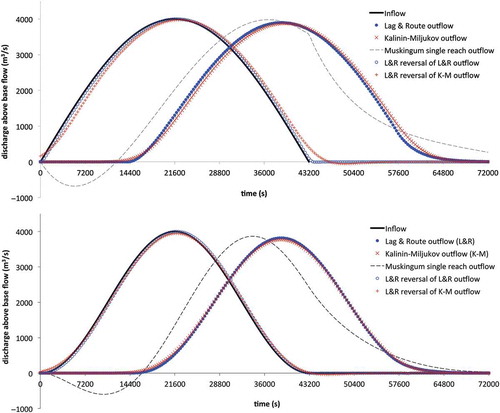
Figure 1. Comparison of the outflow hydrographs of the Lag-and-Route and Kalinin-Miljukov models and of the inflow hydrographs of the reverse Lag-and-Route and Reservoirs-in-Series models: top panel q_in = Q*sinωt and bottom panel q_in = Q*(1 – cosωt)/2; the outflows of the single-reach Muskingum model demonstrate that model’s shortcomings (however, the slope break in the top panel’s hydrograph disappears for the smoother inflow function (1 – cosωt)/2 (bottom panel)).

Bentura and Michel (1997) compared quadratic and linear lag-and-route models, finding that “although the quadratic model clearly outperforms the linear model, the latter remains appealing due to its simplicity and the possibility to highlight, in a very simple way, the interacting roles of the two components of the lag-and-route method. Moreover, it is not certain that the data dealt with in practical applications justify the use of the quadratic model.” In fact, the accuracy of linear models improves when their parameters are made discharge-dependent (Euler and Koussis 1973, Koussis 1978), at the cost of a minor mass balance inconsistency (Koussis 2009); Appendix A outlines a quasi-nonlinear scheme that combines efficiency with accuracy (Koussis and Osborne 1986). Bentura and Michel (1997) discouraged using quasi-nonlinear models in flood forecasting, because this “could come across as risky in the sense that such a method improves the results in ordinary situations but could worsen them in extreme situations or in the vicinity of peaks”. Yet, the need for such caution is less compelling when the range of discharges is known, as routing models can be then suitably referenced to flow rates. Bentura and Michel (1997) also argued that the artificial separation of wave translation and attenuation in the lag-and-route model actually precludes relating its parameters to a physics-based model, and further commented that the bed slope plays an intricate role and that κ_L&R and τ are strongly correlated.

Rearranging the model parameters, Bentura and Michel (1997) formed a new set that they optimised through fitting to a solution ensemble of the St Venant equations, relating them empirically to the bed slope S_o and to Manning’s n of a channel with a wide rectangular cross-section. One parameter of the rearranged lag-and-route parameters set is the time constant κ_L&R + τ that is related to the wave celerity across the reach through L/(κ_L&R + τ). The other parameter of the rearranged set is the ratio τ/(κ_L&R + τ), for which an empirical, best-fit hydro-morphological expression was also obtained. Bentura and Michel (1997), however, did not link the new parameters explicitly to a reference flow rate, which is essential for linear models that hold in a certain flow range. This is, for instance, important for the wave celerity that varies markedly with the discharge. They gave as optimal the fixed value <c_k> = 2.57(√S_o/n)^0.6, which is, presumably, interpreted as applying to all flow rates. However, explicitly linking model parameters to the discharge allows a linear model to be adjusted to the prevailing average flow conditions as needed.

The criticism of Bentura and Michel (1997), that artificially separating wave translation and attenuation in the lag-and-route model precludes strictly relating its parameters to a physics-based model, is indeed theoretically justified. Nevertheless, comparative simulations with the lag-and-route model against linear storage routing models related to the diffusive wave hydraulic model show the former to perform well with the parameters of all models estimated via Dooge’s (1973) method of moment-matching of the SRF to that of the CDE. We therefore accept Dooge’s (1973) optimal parameters for the lag-and-route model, derived by matching its SRF’s first-order moment about the origin and second-order moment about the centroid (the respective first- and second-order cumulants) to those of the CDE’s SRF. The results for a reach length L are understood to relate to a reference flow rate and are as follows (after correcting the mistyped equations (43a, b) in Dooge (1973)):

(12)

(13)

However, a substitute model attains only certain global characteristics of the reference model’s response through moment matching. In the cases of the Muskingum, Kalinin-Miljukov and lag-and-route storage routing models, these characteristics are the centroid translation and the variance (diffusion) of the convective-diffusion wave. Thus, the wave propagations simulated by these models are not identical, varying in certain respects. For instance, the single-reservoir lag-and-route model cannot match the response of n_r reservoirs in series of the Kalinin-Miljukov model, although both have been matched to the SRF’s cumulants of the CDE. Also, for example, the response of the Muskingum model for θ > 0 is negative over a time period 0 < t < t*, while the responses of the Kalinin-Miljukov and lag-and-route models are throughout positive, due to the linear reservoir’s positive SRF (e^–t/k/k). In this particular respect, then, the latter models are exactly CDE-compatible.

3.3 On the time lag τ and its relation to the wave front movement

We discuss here how the lag τ and the travel time of the wave front τ_f may be related, and in Appendix B we check whether the duration of the dip t* is also related to τ. According to the CDE, the wave is a Gaussian profile that spreads while advancing across the reach, its edges moving at infinite speed upstream and downstream. The front of the diffusion wave, however, can be defined and its propagation represented by selecting as half-wave length m standard deviations σ = (2Dτ_f)^1/2, e.g., ±2σ contains approx. 96% of the wave volume. During τ_f then, the wave front advances across the reach length, i.e. L = centroid location + mσ(τ_f) = <c_k>τ_f + m(2Dτ_f)^1/2. Solving this quadratic equation for τ_f yields:

(14)

or, with the characteristic for flood flow Peclet number P ≡ <c_k>L/D,

(14a)

Requiring τ_f = τ yields the number of standard deviations m representing the propagation of a diffusion wave according to the lag-and-route model. This number is obtained via Equations (3) and (12–14), after restating Equation (12) as κ_L&R = [2DL/<c_k>³]^1/2 = (L/<c_k>)(2D/<c_k>L)^1/2 = (L/<c_k>)(2/P)^1/2, and reads (under the assumption that D ≠ 0):

(15)

m(P) varies rapidly as P → 2  [m(2.5)  ≈ 3, m(2.04)  ≈ 10] and slowly for P > 5 [m(5)  ≈ 1.65, m(50)  ≈ 1.1], while m(3.5)  ≈ 2; thus m ≤ 3 fits most cases of practical interest.

These relations lead to the following interpretations of the limiting cases. For the Kalinin-Miljukov unit-reach length L = L_KM = 2D/<c_k>, or P = 2, the lag-and-route model has no channel; it is a single-reservoir Kalinin-Miljukov model. Correctly then, Equation (13) gives as lag τ = 0. In this case m → ∞, by Equation (15): infinite standard deviations σ represent complete (hydraulic) mixing in that reservoir. For D = 0, Equation (12), written as κ_L&R = [2DL/<c_k>³]^1/2, yields κ_L&R = 0; from Equations (13) and (14) then, τ_f = τ  = L/<c_k>: a Dirac pulse travels unchanged at the kinematic wave speed. These results indicate that the lag-and-route model behaves in important global measures consistently with the CDE and therefore is a hydraulically viable flood routing model.

Before proceeding to reverse routing, we benchmark the lag-and-route model against the Kalinin-Miljukov model standard (it allows the finest spatial resolution in storage routing). We reiterate that storage routing models can credibly simulate flood-wave propagation with parameters estimated even from sparse hydro-morphological stream data. Here, we use the uniform channel of Bruen and Dooge (2007) with length L = 100 km, bed slope S_o = 10^–3, Manning’s n = 0.025 and width B = 100 m. The inflow is Q^*sinωt with amplitude Q^* = 4000 m³/s above q_base = 500 m³/s and ω = 2π/T, T = 24 h. At q_o = 2500 m³/s, y_o ≈ 6.28 m and F_o ≈ 0.51, so that D ≈ 11 073 m²/s; linear regression of q(A) over 500 m³/s ≤ q ≤ 5000 m³/s gives <c_k> ≈ 5.8 m/s. The Kalinin-Miljukov unit-reach length is L_KM ≈ 3816 m, thus k = L_KM/<c_k> ≈ 657 s and n_r = L/L_KM ≈ 26; the lag-and-route model parameters are κ_L&R = 3148 s and τ = 14 081 s. In this case, Equation (8) yields analytically (Hoos et al. 1989):

(16)

We also study the case of the slow-rising, concave sinusoid q_in(t) = Q^*[1 – cos(2πt/T)]/2 with T = 12 h. Analytical convolution is possible also in this case, with Equation (8) yielding

(17)

The solutions are obtained by superposing on these responses equal negative ones shifted to t = T. Equations (16) and (17) yield the lag-and-route solutions by setting θ = 0 and K = κ_L&R and by shifting the outflow to t = τ and superposing. In the Kalinin-Miljukov solution (θ = 0 and K = k), the calculation is repeated n_r times numerically. For both inflow signals, the lag-and-route outflow exceeds slightly the Kalinin-Miljukov peak, preceding it by ~300 s; the hydrographs compare well overall (Fig. 1). The outflows of the single-reach Muskingum model [K = κ_L&R + τ = 17 241 s; θ = 0.5 – q_o(1 – p²F_o²)(1 + p)/(3BS_o<c_k>L) ≈ 0.483 (Dooge 1973)] are included for comparison and show the spurious depression, higher peak, and generally markedly different timing and shape.

Finally, we estimate the arrival time of the convection-diffusion wave front at the outflow section by the wave-mechanistic relationship Equation (14a), with m evaluated from Equation (15),

(18)

For <c_k> = 5.8 m/s, L = 100 km and D = 11 073 m²/s, P = 52.4; then, with m = 1.115, τ_f /κ = 0.805; therefore, κ = K = 17 229 s gives τ_f = 13 873 s, merely 1.5% less than the lag τ. This slight discrepancy from the theoretically exact match, τ_f = τ, is due to the fact that Equations (12–15) assume an infinitely wide channel whereas in the calculations here B = 100 m.

4. Reverse storage routing

4.1 The reverse routing models

We consider special inverted numerical forms of the parsimonious lag-and-route model and the fine-resolution cascade of linear reservoirs for stepping back in time. These reverse routing schemes do not suffer the tight grid design restrictions of the inverted Muskingum scheme to control noise amplification (Koussis et al. 2012). The starting point is the reverse procedure of the lag-and-route model (inverted), i.e. reverse-routing the outflow through the linear reservoir and time-shifting it by –τ. In an operational sense, we solve Equation (4), with S = κ_L&R q_out, for an intermediate discharge Q(t) equal to the lagged inflow q_in(t – τ):

(19)

To bring Equation (19) to a form suitable for numerical integration, we discretise in intervals Δt = t_n+1 – t_n, the index n denoting the discretisation level, q_out(t_n) = (q_out)_n (see inset in Fig. 2):

(20)

Figure 2. Reverse routing FD scheme and low-pass filtering—symmetric second-order 11-point filter.

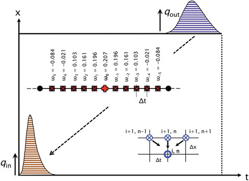
Figure 3. Lag-and-route reverse routing of error-seeded outflow data with filtering (for filter applied only on the outflow data, see inset) and without filtering.

Given discrete outflow values, Equation (20) allows computation of the intermediate discharge Q_n, which is expected to be well-behaved if the outflow data are error-free. Results of reversing error-free outflow data generated (1) analytically and (2) numerically with the lag-and-route model, and (3) numerically by routing with the Kalinin-Miljukov model, show all recovered hydrographs to be close to the analytical inflow. Those corresponding to (2) and (1) are the closest ones, in that order, because in these cases forward and reverse routing are more compatible than in case (3). Figure 1 depicts results for cases (1) and (3).

It is trivially true that Equation (19) would give the exact inflow lagged, if q_out were an error-free analytical solution of κ_L&R dq_out/dt + q_out = Q. What makes Equation (19) attractive for numerical reverse routing is that it allows simple handling of error propagation. Thus, if the data were uncertain, as field data always are, e.g., due to measurement errors, which the derivative dq_out/dt would pass on to Q amplified, the reversed intermediate flow could be conditioned to smooth spurious oscillations, e.g., via a filtering procedure. In reverse routing with the lag-and-route model, filtering would be applied on Q(t) once. In the theoretically more consistent reverse routing approach through n_r linear reservoirs in series, Equation (20) would be applied to each reservoir (κ_L&R = k) with filtering; this computationally more intensive procedure expectedly turned out to be less robust than simple lag-and-route reverse routing.

We consider next the case in which uncertainties, from any source, impair a reliable determination of the outflow, and test the performance of the reverse scheme with error-seeded data. To mimic ‘measured’ outflows q_out|ε(t) (1 + εξ_i), the nominal discrete field data q_out(t) = q(L, t) are seeded with multiplicative random error as follows:

(21)

where ε = % magnitude of error (or error level) and ξ_i = ith standard normal deviate.

Reverse integration of smooth outflow data yields fairly accurate inflow signals (Fig. 1). However, inflows regained via Equation (20) from error-contaminated data exhibit anomalous oscillations, hence data conditioning is needed to control noise amplification and distinguish between true and spurious information. To this end, we applied to the outflow data and to the recovered inflow various Savitzky-Golay low-pass filters, with weights ω_j (Press et al. 1996), Fig. 2:

(22)

However, because low-pass filters do not necessarily preserve the volume of the wave (zero-order moment), minor volume errors are corrected, if needed, by rescaling the recovered inflow to the proper (outflow) volume (Koussis et al. 2012).

Figure 3 shows inflow hydrographs recovered from data seeded with ε = 10% error. Without smoothing, reverse routing increases the perturbations. Good results are achieved with the symmetric, second-order 11-point low-pass filter (weights: w_o = 0.207, w₋₁ = w₁ = 0.196, w₋₂ = w₂ = 0.161, w₋₃ = w₃ = 0.103, w₋₄ = w₄ = 0.021, w₋₅ = w₅ = −0.084) applied to the outflow data and to the recovered inflow hydrograph. Smoothing only the outflow data regains the macro-shape of the inflow hydrograph intact with small roughnesses (see inset). With error-seeded data, the derivative approximation in Equation (20) is more prone to oscillations the smaller the time step Δt is; conversely, as Δt increases, the regained inflow signal becomes smoother but less accurate. In our tests, the signal is recovered well with Δt = 900–1800 s, without rescaling. These tests indicate that low-pass filtering is a simple data-conditioning mechanism that retains much of the physical information intact.

5. Reservoir control

Reservoirs, serving (also) the purpose of flood management, protect downstream areas by controlling the reservoir outflow. In an application involving a reservoir and a flood-relief area adjacent to a river, to which flood waters were diverted via a side-weir, Szöllósi-Nagy (1987) demonstrated that flood control is mathematically identical to signal detection. We consider the operation of a flood protection reservoir. Its outflow is controlled by steering the regular and the flood relief outlet works (spillways or gates), which depends on the hydraulic ratings and the storage characteristics of these structures. In this context, reverse routing can be used to provide information for establishing operational rules based on the reservoir inflows and the desired peak discharge at a target downstream cross-section.

The problem is framed as follows. At a distance L downstream of the reservoir is located an area that must be protected from flood flows in excess of an alarm discharge level q_alarm corresponding to a flood alarm stage. The reservoir releases q(0, t) must be controlled—to the extent feasible—so that the flow at x = L resulting from the flood wave propagation does not exceed a threshold: q(L, t) ≤ q_alarm. The discharge-depth correspondence is not unique in transient flow, it depends on the flow dynamics; however, the q–y threshold relationship may be determined approximately through the Jones-Thomas rating formula q = q_o[1 + (<c_k>S_o)⁻¹ ∂y/∂t]^1/2 by evaluating at-a-section records of water stage or depth (Henderson 1966, Koussis 2010a, 2010b); q_o is a nominal uniform flow rate, in as much as a prismatic channel must be substituted for a natural stream reach to define q_o.

The solution concept is exemplified in Fig. 4 with concrete data and entails the following forward and reverse routing steps: (1) routing the inflow q_in(t) through the reservoir, to predict the (free, uncontrolled) reservoir outflow for a given setting of the outlet works; (2) routing that reservoir outflow to the target stream cross-section at x = L; (3) defining the target flood hydrograph not to exceed q_alarm, e.g., as identical to the hydrograph calculated in step (2) up to the time of occurrence of q(L, t_start) = q_alarm, then remaining at q_alarm until it crosses the hydrograph q(L, t) at t = t_end; and (4) reverse-routing the thus defined q_target(t) to the reservoir, to determine the controlled reservoir outflow hydrograph ensuring q(L, t) ≤ q_alarm. The time-release of the flood volume ΔV stored in the reservoir depends on the steering of the outlet works for t > t_end (for given characteristics of storage vs stage).

Figure 4. Concept of reservoir control with example: controlled reservoir outflows (discharges above baseflow) calculated by the reservoirs-in-series model from filtered (solid line with non-filled circles), and unfiltered (grey solid line) data and by the lag-and-route model (solid line with solid circles) from unfiltered data.

The data of our simplified example are as follows: reservoir constant k_r = 12 h; stream reach length L = 21 100 m, slope S_o = 0.0004, width B = 25 m and Manning’s n = 0.035 (Strickler’s hydraulic conductance 28.6 m^1/3/s). In the flow range up to ~500 m³/s, <c_k> ≈ 2.05 m/s, F_o ≈ 0.2 and D ≈ 9824 m²/s, which give a Kalinin-Miljukov unit-reach length L_KM = 10 543 m, i.e. n_r = 2, and k = L_KM/<c_k≥ 5143 s ≈ 1.4 h. The flood inflow q_in(t) = Q^*[1 – cos(2πt/T)]/2 has amplitude Q^* = 1000 m³/s and cosine period T = 43 200 s = 12 h; stream baseflow is q_base = 42.5 m³/s. The alarm discharge at the cross-section 21.1 km downstream of the reservoir is q_alarm = 250 m³/s, defining t_start = 41 400 s and t_end ≈ 124 200 s in the particular example. The uncontrolled reservoir outflow is calculated analytically with Equation (17) (K = k and θ = 0) and is then routed with the Kalinin-Miljukov method to the target cross-section. The lag-and-route model parameters are τ = 3090 s and κ_L&R = 7202 s.

Figure 4 shows that the reverse calculation, with either model, is able to determine quite properly the controlled outflow hydrograph of the reservoir that ensures the hydrograph at x = L not exceeding the set threshold. The controlled reservoir outflow coincides with the uncontrolled outflow up to close to its maximum and approaches the steady flow limit q_alarm from above. Spurious oscillations appearing in the reverse reservoirs-in-series solution near t_start (grey solid line, Fig. 4) were caused by the discontinuity of dq_out/dt at t_start, as the threshold limits abruptly the curved outflow hydrograph to enforce the steady flow q_out = q_alarm in the time interval [t_start, t_end] (i.e. coincidence of the controlled reservoir outflow and the target hydrograph). By Equation (19), the difference Q – q_out depends on and has the same sign as dq_out/dt. These oscillations all but disappear from the two-reservoir reverse solution (solid line with non-filled circles, Fig. 4), upon filtering three values of q_target(t) just after t_start (t > t_start), to eliminate the slope break at t_start. The inverted lag-and-route solution (solid line with solid, black circles, Fig. 4) is robust and was obtained without filtering. The target hydrograph is recovered when the controlled reservoir outflow is routed to the section at x = L = 21.1 km, indicating the correctness of the reverse control procedure.

6. Pollution routing

The inverted routing models presented here may be also applied to reverse concentration routing (Koussis et al. 2012), based on the fact that the CDE is the common mathematical basis of flood routing and 1-D pollutant transport (Koussis 1983, Koussis et al. 1983), i.e. Equation (1) holds with q replaced by the concentration C, the kinematic wave celerity c_k by the mean cross-sectional velocity V of steady flow and the hydraulic diffusion coefficient D by the longitudinal dispersion coefficient D_L. We demonstrate reverse mass transport by comparing the results in Fig. 5 of the lag-and-route model with the data for cross-sections 4 and 6 of Test 6 of the field experiment of Godfrey and Frederick (1970) in Copper Creek, Virginia, compiled in their Table 10A.

Figure 5. Pollutographs (C): observed (black dots) C_in and breakthrough curves, and lag-and-routed forward (L&R) (+) and reverse recovered (empty circles) curves.

The transport parameters V and D_L of the stream reach, of length L = 1732 m, were first identified by forward lag-and-routing. Routing through the linear reservoir was carried out with the Kalinin-Miljukov scheme (also, exponential Muskingum scheme with θ = 0, see Appendix B), which assumes a linear variation of the hydrograph/pollutograph over a time step Δt (in this case, of variable duration): (C_out)_n+1 = a₁(C_in)_n + a₂(C_in)_n+1 + a₃(C_out)_n, where, with C_o = Δt/κ_L&R, a₁ = C_o^–1(1 – e^−C_o) – e^−C_o, a₂ = 1 – C_o⁻¹(1 – e^−C_o), a₃ = e^−C_o; a₁ + a₂ + a₃ = 1. However, we noticed that total solute was not conserved; the areas under the pollutographs are unequal, 1646 vs 1299 μCurie/ft³ s (× the volumetric flow rate = total solute); a likely reason for these losses is trapping or sorption of the solute in streambed sediments and/or channel irregularities and groins (Fischer et al. 1979, p. 109–112). Therefore, we accounted for the loss of solute approximately by rescaling the lag-and-routing results by 1299/1646 = 0.789, reducing the calculated values (in reverse routing, the inverted concentrations were increased similarly). Forward routing then gave the fit shown in Fig. 5 and Table 1, with the following parameters: τ = 2301 s = 38.35 min and κ_L&R = 765 s = 12.75 min, corresponding to V = 0.565 m/s and D_L = 30.45 m²/s.

Table 1. Concentrations calculated forward and reverse with the lag-and-route model.

Time relative to 11:49 (min)	Cin = C(t, x = 0) from reverse routing (μCi/ft^3)	Time relative to 11:49 (min)	Cout = C(t, x = L) from forward routing (μCi/ft^3)
−1.35	0	38.35	0
3.65	0.444	41.35	0.022
8.65	0.812	44.35	0.096
13.65	1.000	47.35	0.210
17.65	0.997	49.35	0.297
21.65	0.937	51.35	0.381
23.65	0.788	53.35	0.454
25.65	0.647	55.35	0.510
29.65	0.468	57.35	0.550
36.65	0.290	62.35	0.583
45.65	0.085	67.35	0.548
55.65	0.008	72.35	0.473
65.65	−0.013	77.35	0.385
		87.35	0.234
		97.35	0.127
		107.35	0.062
		117.35	0.028
		127.35	0.013
		132.35	0.009
		135.35	0.007

Further, to accommodate the unevenly spaced observations, the derivative in Equation (19) at time t_n (restated here in terms of concentrations) was approximated by weighing equally the forward and the backward differences over the respective intervals Δt_n/n+1 and Δt_n/n-1, obtaining the first-order accurate inversion scheme for the intermediate concentration value at the inflow section prior to the lag-step, c_in(t) = C_in(t – τ), from which the second-order accurate scheme of Equation (20) is regained for Δt_n/n+1 = Δt_n/n-1 = Δt:

(23a)

(23b)

The results of Equation (23) were finally lagged and rescaled to yield the inflow pollutograph shown in Fig. 5 and Table 1; filtering was not applied because the breakthrough curve is quite smooth. The modest precision in the peak region of C_in(t) is due in part to inadequate resolution of the breakthrough curve in the range 47–60 min after the initiation of the experiment, the time interval yielding the high inflow concentrations after inversion of the data. The zero-point of the inflow pollutograph determined through reverse routing, −1.35 min, was obtained by subtracting τ from the zero-concentration time of the breakthrough curve, 37 min, and is fairly close to relative time zero.

7. Discussion

All models are subject to limitations, because they are incomplete replicas of physical reality (imperfect model structure); e.g., the St Venant hydraulic equations describe transient open-channel flow only in one dimension under simplifying assumptions, such as, e.g., hydrostatic pressure (Koussis (1975) gives a rigorous derivation). Additionally, in field applications, the model parameters and/or the channel morphology are only partially known, the latter inevitably impacting spatial resolution of the simulations, especially with complete hydraulic models. Furthermore, observations are always affected by inaccurate measurements and possibly by errors. As a result of these shortcomings, difficulties and associated uncertainties, it is important that a model be robust. A parsimonious model structure is a virtue in this respect, as is a simple routing scheme that allows a transparent numerical treatment of data errors, as well as an efficient calculation.

The adequacy of wave propagation simulations by storage routing models is a prime issue. To this, we reiterate (Section 3.1) that storage routing models have been field-verified and owe their success to the fact that, properly applied, they are akin to the CDE, and thus approximate the hydraulic equations well across a wide range of conditions (e.g., Koussis 2009). As stated in Section 3.1, the fundamental limitation of storage routing models derives from being upstream-controlled CDE substitutes (Koussis 2009, 2010a), and hence incapable of accommodating a downstream boundary condition. That aside, with proper parameters, they can treat even pronounced transients on mild slopes, i.e. those generating at a cross-section depth (stage) vs discharge curves with sizeable loops; the degree of transience can be gauged by the slope ratio SR = −∂y/∂x/S_o ≈ ∂y/∂t/c_kS_o (Koussis and Chang 1982). A conservative limit for storage routing applications is SR ≤ 0.5, but transients with SR ≈ 1 have been handled successfully too (Koussis 2010b). In such cases the kinematic wave celerity c_k = dq/dA|_{x = const.} should be determined iteratively as the slope of the rating curve approximation of Jones-Thomas q(t) = q_o[1 + (<c_k>S_o)⁻¹ ∂y/∂t]^1/2 = q_o[1 + (B<c_k>²S_o)⁻¹ ∂q/∂t]^1/2 (Koussis 1975, Koussis 2009, 2010a, 2010b, Weinmann 1977, Weinmann and Laurenson 1979, Perkins and Koussis 1996). Regarding the calculation of depths, the local character of depth must be noted. Depth is affected by the local stream morphology (Koussis 2010b); therefore, it can be calculated reliably via the differential volume balance ∂A/∂t + ∂q/∂x = 0 only if detailed morphological data are available. In contrast, discharge varies more regularly (the peak flow rate always decreases downstream, but not the morphology-dependant peak depth). Thus, after routing with parameters that can be estimated even from fairly sparse morphological data (better, also calibrated against flood data), depths can be determined from the rating curves (steady- or transient-state) at the end-sections of the reach. In general, storage routing of discharges is robust, i.e. results are not over-sensitive to suboptimal parameter values, a trait inherited by reverse routing. In addition, the high computational efficiency of reverse routing permits carrying out readily multiple runs that may be used to assess uncertainties in a reverse ensemble forecasting sense.

The performance of the lag-and-route model, in reverse and in forward modes, confirms the effectiveness of the concept. Dooge (1973) was probably the first to suggest extending that concept, by adding a lag to a series of linear reservoirs, to improve routing accuracy. Adopting Dooge’s idea, Camacho and Lees (1999) demonstrated its utility using the linearisation-based parameter estimation through cumulants matching of Dooge et al. (1987a, 1987b) for a “generalised uniform channel” of any cross-sectional shape. They also showed that the number of reservoirs is drastically reduced relative to a cascade model without a lag element, but that, then, the routing time step must be smaller and may result in considerable execution times, especially for dynamic waves in irregular channels (those with wide-loop rating curves). Camacho and Lees (1999) also found that a quasi-nonlinear modelling approach (Appendix A) improves accuracy, in agreement with Wang and Singh’s (1992) further development of variable-parameters concepts (Euler and Koussis 1973, Koussis 1975, 1976, 1978, Ponce and Yevjevich 1978, Ponce 1979). The straightforward extension to “generalised uniform channels” and the refinement of the quasi-nonlinear approximation could be readily applied also in reverse routing. We did not implement them in this work because we intended to demonstrate as clearly as possible the feasibility of solving a difficult signal identification problem by relatively simple methods.

Regarding the reservoir control problem, it should be noted that an approximate heuristic solution is to simply limit the uncontrolled reservoir outflow hydrograph at the discharge q_alarm. In that case the approach to the hydrograph threshold at the target cross-section would occur somewhat later and more flood volume would have to be stored inside the reservoir. In the particular example, the difference between the complete and the approximate heuristic solution is small, because the distance to the target stream cross-section is relatively short (21 km) and, as a result, the portion of the outflow hydrograph above q_alarm is also small. For longer reaches, however, both the base of the triangle-like part of the hydrograph and its peak over q_alarm increase. These changes occur then, because t_start occurs later (the uncontrolled q(L, t) at the end of a longer reach starts later) and at that time the discharge of the uncontrolled-reservoir outflow above the limiting value q_alarm of the target q(L, t) increases, leading to a higher peak of the controlled-reservoir outflow.

Various low-pass filters were used in the test cases considered. These filters were selected empirically by trial and error, depending on the problem at hand. For example, the symmetric, second-order 11-point Savitzky-Golay low-pass filter (Press et al. 1996) was able to recover a smooth and mass-conserving (no rescaling) inflow hydrograph with the lag-and-route reverse routing model from the error-seeded outflow hydrograph shown in Fig.3, while the symmetric, second-order, five-point low-pass filter, used by Koussis et al. (2012) in connection with reverse Muskingum routing, and the 9-point and 11-point fourth-order symmetric low-pass filters, did not smooth the data equally well. In contrast, a simple filter was sufficient to handle the break in the hydrograph slope in the case of the reservoir control example and no filtering was necessary in the reverse pollution routing field case. Based on this limited experience, we expect the choice of an appropriate filter to depend on the noise of the signal data (error level and frequency). In real-world applications, appropriate filters can be test-chosen using available observations.

Applying the inverted lag-and-route model to one-dimensional solute transport in streams demonstrated some of the difficulties arising in actual field cases, such as violation of mass conservation and data sampling in variable time intervals, which were handled by ad hoc procedures. We note that in this particular case a cells-in-series transport model (equivalent to the Kalinin-Miljukov flood routing model) would have n_r ≈ 16 cells (reservoirs), in stark contrast to the parsimonious (single-cell) lag-and-route equivalent transport model. An advantage of the particular numerical schemes Equations (20) and (23) is that they identify the lagged signal, Q or c_in, based only on q_out or C_out data; signal values identified in previous reverse steps, which would carry perturbations, are not present. In contrast, the reverse Muskingum box routing scheme (Koussis et al. 2012), by involving in- and outflow values at the current and at the next (or previous) time levels, includes also a previously identified signal value that makes it sensitive to error propagation. Finally, the modestly resolved breakthrough curve in the range 12:36–12:49 led to the dilemma of using either the only first-order accurate scheme with the actual data or the second-order accurate scheme with data interpolated linearly at constant intervals. We chose the first option, considering it essential to work with the actual data, but tested the second option as well, which proved inferior. The partially artificial data, due to the linear interpolation in the range of relative time 50–64 min (usually acceptable, but questionable in error-sensitive reverse calculations), caused the results near the peak to fluctuate mildly (not shown).

8. Summary and conclusions

Key to the performance of the inverted routing scheme is its simple structure. The centred FD approximation of the storage balance equation for a linear reservoir involves only one value of the unknown signal; signal values identified in previous reverse steps, which would carry perturbations, are absent. This structure endows the reverse scheme with robustness also regarding grid design. Synthetic tests, with perfect and with error-seeded data (mimicking field observations), resulted in good signal recovery very efficiently, verifying the effectiveness of the developed reverse routing procedures. These procedures are complemented, if needed, by low-pass filtering, to damp oscillations in the solution caused by errors or discontinuities in the initial data.

Reverse storage routing was exemplified in a reservoir-control study for flood protection. In that case, filtering of three data points sufficed to damp oscillations caused by a discontinuity of the first derivative of the outflow hydrograph, to which the reservoirs-in-series reverse model was more prone than the inverted lag-and-route model. Reverse lag-and-routing also performed well without filtering in an application of mass transport in a stream with partly sparse and unevenly sampled data. Parsimony, robustness—both attributed to the scheme’s particular and simple structure—and good accuracy recommend the inverted lag-and-route model for reverse routing, perhaps over the theoretically superior, but more complex and sensitive inverted reservoirs-in-series model. Finally, the particular scheme’s high efficiency makes reverse storage routing suitable for error assessment in a stochastic framework such as, e.g., ensemble hind-casting (reverse-mode forecasting).

The hydraulic basis of the lag-and-route model was investigated and a wave-mechanistic interpretation of the lag was given in terms of the movement of the diffusion wave front. In Appendix B, it is shown that the duration of the dip of the single-reach Muskingum model is closely related to the lag only in the case of a linearly rising inflow hydrograph near t = 0. Appendix A also confirms that explicit quasi-nonlinear routing schemes can offer good approximations of nonlinear routing solutions very efficiently.

Disclosure statement

No potential conflict of interest was reported by the authors.

Appendix A: Nonlinear and quasi-nonlinear routing schemes

Nonlinear models have flow-independent parameters related to the hydro-morphology of a channel; however, nonlinear routing schemes are complex. For example, the quadratic lag-and-route model, q ∝ S² (Bentura and Michel 1997), allows solving the storage balance equation analytically for constant inflow, but the routing scheme must be iterated repeatedly in a time step. In addition, the analytically convenient quadratic storage model is at some variance with open-channel hydraulics, according to which S = Cq^m with 0.6 ≤ m < 1; e.g., m = 3/4 for channels of triangular cross-section and m = 0.6 for an infinitely wide channel (Koussis 2009). Quasi-nonlinear models are attractive, because they approach the performance of nonlinear models retaining the efficiency of linear routing (Koussis and Osborne 1986). Consider then the nonlinear storage–outflow relationship

(A1)

Using Equation (A1) in the storage balance Equation (4), dS/dt = q_in – q_out, discretised with the trapezoidal rule in a time interval Δt = t_n+1 – t_n, yields the implicit routing scheme:

(A2a)

(A2b)

where F_n/n+1 includes the known discharge terms. Point iteration on Equation (A2a,b) converges for Δt ≥ 2Cm(q_out)^m–1 (Koussis and Osborne 1986). For m = 1, equation (A2a,b) reverts to the explicit, traditional Muskingum routing scheme with θ = 0. For m = 1/2 and m = 2, Equation (A2a,b) becomes quadratic and is solvable analytically, free of a stability constraint. The quadratic equation for m = 1/2 is fairly compatible with open-channel hydraulics and reads in the simplified notation Q ≡ (q_out)_{n + 1} and F ≡ F_n/n + 1, Q²  –  (4/a² + 2 F)Q + F² = 0, where a = Δt/2C. For convenience of demonstration, however, we choose m = 2 and obtain the simpler quadratic:

(A3)

The physically meaningful root of this equation is:

(A4)

The accuracy of the numerical procedure is benchmarked against the exact analytical solution of Ding (1974) for a negative-step inflow from a steady flow q_in = q_out = q_o at t = 0 to q_in(t > 0) = 0 that is valid for m ≠ 1 and reads:

(A5)

Ding’s solution is restated in non-dimensional form as Q/q_o = 1 – ζ/2 for m = 2, with ζ = t/Cq_o; the non-dimensional form of the numerically derived Equation (A4) is Q/q_o = (Δζ/4)[–1 + (1 + 8 F/Δζq_o)^1/2]. The step change constitutes an arduous test for a discrete scheme, yet Fig. A1 verifies that Equation (A4) with Δζ ≤ 0.05 yields a solution in excellent agreement with the analytical Equation (A5) (the accuracy of the integration is still good even with Δζ = 0.10).

Figure A1. Comparison of numerical quasi-nonlinear solution to Ding’s analytical solution.

We also summarise key findings of a test comparing nonlinear and quasi-nonlinear routing through a nonlinear (m = 2/3) quasi-distributed storage element (θ ≠ 0) (Koussis and Osborne 1986). Quasi-nonlinear routing was executed with the Muskingum scheme, m = 1, with discharge-dependent K(q) = L/<c_k(q)> where either q = q₃ = [(q_in)_n + (q_in)_n+1 + (q_out)_n]/3 or q = q₄ = [(q_in)_n + (q_in)_n+1 + (q_out)_n + (q_out)_n+1]/4. The routing scheme is explicit with q = q₃ and implicit with q = q₄ (requiring iterations, without however achieving better accuracy); the mean error of both quasi-nonlinear solutions relative to the nonlinear solution was ε ≈ 0.1% (ε ≈ 3% for linear routing). However, the θ–generalised version of Equation (A2a,b) converged in ~6 times more iterations than the implicit quasi-nonlinear router. All schemes conserved mass very well.

Appendix B: Is the lag τ related to the duration of outflow dip in Muskingum routing?

The lag τ cannot be linked rigorously to the duration of the dip t* that depends on q_in(t) and thus is not a system characteristic. It is nevertheless of interest to test whether an approximate τ–t* relationship exists. Representing the inflow hydrograph near t = 0 by q_in(t) = at and setting q_out(t) = 0 in Equation (8) yield the following implicit equation for t*:

(B1)

Solving Equation (B1) with K = κ_L&R + τ = 17 229 s and θ = 0.5 – q_o(1 – p²F_o²)(1 + p)/(3BS_o<c_k>L)  ≈ 0.483 (Section 3.3) yields t* = 13 414 s. Chang et al. (1983, 1984a, 1984b)) derived Equation (B1) in determining the minimum Δt for skipping over the dip in routing with the exponential Muskingum scheme (Nash 1959, Seus and Rösl 1972, Koussis 1975, 1978, 1980, 2009, Weinmann 1977, Weinmann and Laurenson 1979, Ferrick et al. 1984, Bowen et al. 1989). However, the θ–value for the exponential routing scheme (matching numerical and physical diffusion coefficients) is θ_exp = 1 – C_o /{ln[(1 + C_o + 2/P_Δ)/(1 – C_o + 2/P_Δ)]}  ≈  0.55, where C_o = < c_k>Δt/Δx = Δt/K the Courant number and P_Δ = < c_k>Δx/D the grid Peclet number (Koussis 2009), and gives t* = 14 649 s. Both these t*-values are close to the lag τ = 14 091 s, approx. ±4.5%. (In contrast, the fractional Muskingum scheme, which ignores the inflow shape (Chang et al. 1983, 1984a, 1984b), gives t* = 2 Kθ = 16 658 s, ~18.5% over τ).

Yet such agreement is not general; if for instance q_in = at², setting q_out = 0 in Equation (8) yields:

(B2)

with the root (satisfying τ < K as per Equation (13)) t* ≈ 11 620 s for θ = 0.483 (~17.5% less than τ). Furthermore, for the rapidly rising, convex (half-)sine q_in(t) = Q^*sin(2πt/T) with T = 24 h, setting q_out = 0 in Equation (16) yields t* ≈ 12 000 s (~15% less than τ). For the slow-rising, concave sinusoid q_in(t) = Q^*[1 – cos(2πt/T)]/2 with T = 12 h, Equation (8) yields analytically Equation (17), from which one obtains t* ≈ 16 200 s (~15% greater than τ) by setting q_out = 0.

Hence, the lag of the lag-and-route model and the duration of the outflow dip of the single-reach Muskingum model are close (±4.5%) only if the inflow is linear near t = 0; if the inflow rises slowly (under-linearly) t* > τ, and if it rises rapidly (over-linearly) t* < τ.

References

- Bentura, P.L.F. and Michel, C., 1997. Flood routing in a wide channel with a quadratic lag-and-route method. Hydrological Sciences Journal, 42 (2), 169–189. doi:10.1080/02626669709492018
- Bowen, J.D., Koussis, A.D., and Zimmer, D.T., 1989. Storm drain design diffusive flood routing for PCs. Journal of Hydraulic Engineering ASCE, 115 (8), 1135–1150. doi:10.1061/(ASCE)0733-9429(1989)115:8(1135)
- Bronstein, I.N. and Semendjajew, K.A., 1964. Taschenbuch der Mathematik. Zürich: Verlag Harri Deutsch.
- Bruen, M. and Dooge, J.C.I., 2007. Harmonic analysis of the stability of reverse routing in channels. Hydrology and Earth Systems Sciences, 11 (1), 559–568. doi:10.5194/hess-11-559-2007
- Camacho, L.A. and Lees, M.J., 1999. Multilinear discrete lag-cascade model for channel routing. Journal of Hydrology, 226, 30–47. doi:10.1016/S0022-1694(99)00162-6
- Chang, C.-N., Da Motta Singer, E., and Koussis, A.D., 1983. On the mathematics of storage routing. Journal of Hydrology, 61 (4), 357–370. doi:10.1016/0022-1694(83)90001-X
- Chang, C.-N., Da Motta Singer, E., and Koussis, A.D., 1984a. On the mathematics of storage routing – reply. Journal of Hydrology, 69, 365–366. doi:10.1016/0022-1694(84)90175-6
- Chang, C.-N., Da Motta Singer, E., and Koussis, A.D., 1984b. On the mathematics of storage routing – reply. Journal of Hydrology, 73, 395–397. doi:10.1016/0022-1694(84)90012-X
- Ding, J.Y., 1974. Variable unit hydrograph. Journal of Hydrology, 22, 53–69. doi:10.1016/0022-1694(74)90095-X
- Dooge, J.C.I., 1973. Linear theory of hydrologic systems. Washington DC: Agricultural Research Service, US Department of Agriculture, Tech. Bull. no. 1468.
- Dooge, J.C.I., Napiorkowski, J.J., and Strupczewski, W.G., 1987a. The linear downstream response of a generalised uniform channel. Acta Geophysica Polonica, 35 (3), 277–291.
- Dooge, J.C.I., Napiorkowski, J.J., and Strupczewski, W.G., 1987b. Properties of the generalised downstream channel response. Acta Geophysica Polonica, 35 (4), 405–418.
- D’Oria, M., Mignosa, P., and Tanda, M.G., 2014. Bayesian estimation of inflow hydrographs in ungauged sites of multiple reach systems. Advances in Water Resources, 63, 143–151. doi:10.1016/j.advwatres.2013.11.007
- D’Oria, M. and Tanda, M.G., 2012. Reverse flow routing in open channels: a Bayesian geostatistical approach. Journal of Hydrology, 460–461, 130–135. doi:10.1016/j.jhydrol.2012.06.055
- Eli, R.N., Wiggert, J.M., and Contractor, D.N., 1974. Reverse flow routing by the implicit method. Water Resources Research, 10 (3), 597–600. doi:10.1029/WR010i003p00597
- Euler, G. and Koussis, A., 1973. Berechnung von Hochwasserablaeufen mit Naeherungsverfahren und ihre Anwendung. Die Wasserwirtschaft, 63 (8), 235–240.
- Ferrick, M.G., Blimes, J., and Long, S.E., 1984. Modeling rapidly varied flow in tailwaters. Water Resources Research, 20 (2), 271–289. doi:10.1029/WR020i002p00271
- Fischer, H.B., et al., 1979. Mixing in Inland and coastal waters. San Diego, CA: Academic Press.
- Godfrey, R.G. and Frederick, B.J., 1970. Stream dispersion at selected sites. Washington, DC: U.S. Dept of the Interior. USGS Professional Paper 433-K.
- Henderson, F.M., 1966. Open channel flow. New York: Macmillan.
- Hoos, A.B., Koussis, A.D., and Beale, G.O., 1989. A channel dynamics model for real-time flood forecasting. Water Resources Research, 25 (4), 691–705. doi:10.1029/WR025i004p00691
- Kalinin, G.P. and Miljukov, P.I., 1958. Approximate methods for computing unsteady flow movement of water masses (in Russian). Transactions Central Forecasting Institute, 66.
- Koussis, A., 1975. Ein Verbessertes Näherungsverfahren zur Berechnung von Hochwasser-abläufen (An improved approximate flood routing method, in German). Darmstadt: Institut für Hydraulik und Hydrologie, Technische Hochschule Darmstadt, Technical Report no. 15.
- Koussis, A., 1976. An approximative dynamic flood routing method. In: H.S. Stephens, S.K. Hemmings, BHRA, IAHR, eds. International symposium on unsteady flow in open-channels proceedings, 1976 Newcastle-Upon-Tyne. Cranfield: BHRA Fluid Engineering, Paper L1.
- Koussis, A. and Chang, C.-N., 1982. Efficient analysis of storm drain networks. In: B.C. Yen, ed. Urban stormwater hydraulics and hydrology. Littleton, CO: Water Resources Publication LLC, 314–322.
- Koussis, A.D., 1978. Theoretical estimations of flood routing parameters. Journal of the Hydraulics Division ASCE, 104 (HY1), 109–115.
- Koussis, A.D., 1980. Comparison of Muskingum method difference schemes. Journal of the Hydraulics Division ASCE, 106 (HY5), 925–929.
- Koussis, A.D., 1983. Unified theory for flood and pollution routing. Journal of Hydraulic Engineering ASCE, 109 (12), 1652–1664. doi:10.1061/(ASCE)0733-9429(1983)109:12(1652)
- Koussis, A.D., 2009. An assessment review of the hydraulics of storage flood routing 70 years after the presentation of the Muskingum method. Hydrological Sciences Journal, 54 (1), 43–61. doi:10.1623/hysj.54.1.43
- Koussis, A.D., 2010a. Reply to the Discussion of “An assessment review of the hydraulics of storage flood routing 70 years after the presentation of the Muskingum method” by M. Perumal. Hydrological Sciences Journal, 55 (8), 1431–1441. doi:10.1080/02626667.2010.491261
- Koussis, A.D., 2010b. Comment on “A praxis-oriented perspective of streamflow inference from stage observations – the method of Dottori et al. (2009) and the alternative of the Jones Formula, with the kinematic wave celerity computed on the looped rating curve”. Hydrology and Earth Systems Sciences, 14, 1093–1097. doi:10.5194/hess-14-1093-2010
- Koussis, A.D. and Osborne, B.J., 1986. A note on nonlinear storage routing. Water Resources Research, 22 (13), 2111–2113. doi:10.1029/WR022i013p02111
- Koussis, A.D., Saenz, M.A., and Tollis, I.G., 1983. Pollution routing in streams. Journal of Hydraulic Engineering ASCE, 109 (12), 1636–1651. doi:10.1061/(ASCE)0733-9429(1983)109:12(1636)
- Koussis, A.D., et al., 2012. Reverse flood routing with the inverted Muskingum storage routing scheme. Natural Hazards and Earth System Sciences, 12 (1), 217–227. doi:10.5194/nhess-12-217-2012
- Leonhardt, G., et al., 2014. Comparison of two model based approaches for areal rainfall estimation in urban hydrology. Journal of Hydrology, 511, 880–890. doi:10.1016/j.jhydrol.2014.02.048
- Lighthill, M.J. and Whitham, G.B., 1955. On kinematic waves I. Flood movement in long rivers. Proceedings of the Royal Society of London, Series A, Mathematical and Physical Sciences, 229 (1178), 281–316. doi:10.1098/rspa.1955.0088
- Mazi, K. and Koussis, A.D., 2010. Reverse flood routing with the lag-and-route storage model. In: 12th Plinius conference on mediterranean storms September, Corfou.
- Meyer, O.H., 1941. Simplified flood routing. Journal of Civil Engineering Division ASCE, 11 (5), 306–307.
- Nash, J.E., 1959. A note on the Muskingum flood-routing method. Journal of Geophysical Research, 64 (8), 1053–1056. doi:10.1029/JZ064i008p01053
- Perkins, S. and Koussis, A., 1996. Stream-aquifer interaction model with diffusive wave routing. Journal of Hydraulic Engineering, 122 (4), 210–218. doi:10.1061/(ASCE)0733-9429(1996)122:4(210)
- Ponce, V.M., 1979. Simplified Muskingum routing equation. Journal of the Hydraulics Division ASCE, 105 (HY1), 85–91.
- Ponce, V.M. and Yevjevich, V., 1978. The Muskingum-Cunge method with variable coefficients. Journal of the Hydraulics Division ASCE, 104 (HY12), 1663–1667.
- Press, W.H., et al., 1996. Numerical recipes in FORTRAN 77: the art of scientific computing. 2nd ed. New York: Cambridge University Press.
- Reggiani, P., Todini, E., and Meissner, D., 2014. A conservative flow routing formulation: Déjà vu and the variable-parameter Muskingum method revisited. Journal of Hydrology, 519, 1506–1515. doi:10.1016/j.jhydrol.2014.08.057
- Seus, G.J. and Rösl, G., 1972. Hydrologische Verfahren zur Berechnung des Hochwasserwellen- ablaufs in Flüssen. In: W. Zielke, ed. Elektronische Berechnung von Rohr- und Gerinneströmungen. Berlin: Erich Schmidt Verlag.
- Strupczewski, W. and Kundzewicz, Z., 1980. Translatory characteristics of the Muskingum method of flood routing—a comment. Journal of Hydrology, 48, 363–368. doi:10.1016/0022-1694(80)90126-2
- Szöllósi-Nagy, A., 1987. Input detection by the discrete linear cascade model. Journal of Hydrology, 89, 353–370. doi:10.1016/0022-1694(87)90186-7
- Szymkiewicz, R., 1996. Numerical stability of implicit four-point scheme applied to inverse linear flow routing. Journal of Hydrology, 176, 13–23. doi:10.1016/0022-1694(95)02785-8
- Venetis, C., 1969. The IUH of the Muskingum channel reach. Journal of Hydrology, 7, 444–447. doi:10.1016/0022-1694(69)90097-3
- Wang, G.-T. and Singh, V.P., 1992. Muskingum method with variable parameters for flood routing in channels. Journal of Hydrology, 134, 57–76. doi:10.1016/0022-1694(92)90028-T
- Weinmann, P.E., 1977. Comparison of flood routing methods in natural rivers. Victoria, Australia: Department of Civil Engineering, Monash University Clayton, Report no. 2/1977
- Weinmann, P.E. and Laurenson, E.M., 1979. Approximate flood routing methods: a review. Journal of the Hydraulics Division ASCE, 105 (12), 1521–1536.