Application of Fourier series in managing the seasonality of convective and monsoon rainfall

ABSTRACT

This study assesses the performance of Fourier series in representing seasonal variations of the tropical rainfall process in Malaysia. Fourier series are incorporated into a spatial-temporal stochastic model in an attempt to make the model parsimonious and, at the same time, capture the annual variation of rainfall distribution. In view of Malaysia’s main rainfall regime, the model is individually fitted for two regions with distinctive rainfall profiles: one being an urban area receiving rainfall from convective activities whilst the other receives rainfall from monsoonal activities. Since both regions are susceptible to floods, the study focuses on the rainfall process at fine resolution. Fourier series equations are developed to represent the model’s parameters to describe their annual periodicity. The number of significant harmonics for each parameter is determined by inspecting the cumulative fraction of total variance explained by the significant harmonics. Results reveal that the number of significant harmonics assigned for the parameters is slightly higher in the region with monsoonal rains. The overall simulation results show that the proposed model is capable of generating tropical rainfall series from convective and monsoonal activities.

Editor D. Koutsoyiannis Associate editor K. Hamed

KEYWORDS:

• Fourier series
• significant harmonic
• annual variation
• convective
• monsoon

1 Introduction

The rainfall process results from the interaction of several complex elements of the atmospheric process. This intricate activity causes rainfall distributions to vary between locations, season to season and year to year. Factors contributing to the variations include the local climate and geographical and topographical conditions. For example, spatial and temporal variations of rainfall distribution in tropical regions are significantly higher than those in temperate regions. Countries of substantial size, such as the United States, Australia, Russia and China, have very prominent spatial variations.

Rainfall data are the key input in a variety of hydrological applications; however, lack and insufficiency of available data lead to the increased use of rainfall models to synthetically generate data. Since the rainfall process varies in time and space, rainfall models must be able to absorb and represent these variations. With regard to temporal variations, rainfall models normally employ different sets of parameters at different times of the year, for instance according to seasons or according to months. For spatial variations, different parameters are assigned at different locations within a large area. However, by employing these different sets of parameters, rainfall models end up with too many parameters. To capture these variations while keeping the models parsimonious, a technique often incorporated into the models is the harmonic analysis of Fourier series.

Harmonic analysis of Fourier series is a technique of decomposing the whole time series into infinite series of harmonic components and an additive term (Davis 1986). Each component consists of sine and cosine waves where the two waves are merged into a single cosine wave. Each wave has its own amplitude (wave size) and phase angle (offset of wave). The additive term is used to assign the number of complete cycles by a wave over some defined interval. For example, the third term indicates there are three complete cycles. Every component accounts for a certain proportion of the total variance in the initial dataset.

Well-known applications of the composition of sine and cosine waves include those by Bernoulli (1700–1782) in vibrating string studies and Euler (1707–1783) in astronomy. Later, Joseph Fourier (1768–1830) notably expanded and revolutionized the theoretical principles of the sine and cosine waves to solve problems concerning heat conduction. Today, the series, named the Fourier series, facilitates solving a wide range of practical engineering and science problems. Examples of hydrological applications include studies on rainfall (Guenni et al. 1996, Machiwal and Jha 2008) and streamflow (Bayazit et al. 2001). In rainfall studies, available literature shows the applications of Fourier series mainly fall into two categories. The first applies Fourier series to investigate the pattern of spatial variation of the rainfall process within a large study region. In such studies, Fourier series are used to describe and delineate boundaries according to some characteristics (i.e. amount, mean or standard deviation) of the rainfall process. Sabbagh and Bryson (1962) used the series to define regional boundaries of the different rainfall regimes in Canada. Similar studies were conducted by Fitzpatrick (1964) in Australia, and by Kirkyla and Hameed (1989) in the United States. There are also studies that incorporated Fourier series in representing spatial variations of the model parameters. Transform models are used to simulate rainfall series within a fitted region. Woolhiser and Roldán (1986) employed this technique to represent parameters of a first-order Markov chain model, while Hutchinson (1991) adopted it for an alternating renewal model.

The second category focuses on the use of Fourier series in representing seasonal variations of the rainfall process throughout the year. Advocates of such an approach include Woolhiser and Pegram (1979), who incorporated Fourier series to represent the seasonal variation of parameters of a two-state Markov chain model for rainfall occurrence while a mixed exponential distribution was used to represent rainfall amount. The parameters of the Markov chain were estimated using the maximum likelihood method and were then transformed to Fourier series equations. In studies by Stern and Coe (1984), the parameters of the generalized linear model were represented by Fourier series equations. Similarly, Guenni et al. (1996) fitted Fourier series to the parameters of the rectangular pulse Poisson model, while Fadhilah et al. (2008) employed them to represent the parameters of the single-site Neyman-Scott rectangular pulse model.

In this study, the goal is to investigate the use of Fourier series in a stochastic model to address the need for a parsimonious rainfall model whilst taking into consideration the annual variation of the tropical rainfall process. Specifically, the spatial-temporal Neyman-Scott rectangular pulse (STNS) model is chosen to generate hourly rainfall series for two regions in Peninsular Malaysia. Previous studies (Cowpertwait and Kilsby 2002, Leonard et al. 2007) showed that this space-time model is able to adequately represent rainfall processes at different time scales. The STNS model is stationary; however, Malaysia’s tropical climate exhibits distinctive month to month variations of rainfall distribution (Syafrina et al. 2014a). Thus it is necessary to allow the parameters of the STNS model to vary throughout the year by estimating each parameter on a monthly basis. Nevertheless, having 12 sets of parameters per year often leads to overfitting and abrupt changes between months. To compensate for this shortcoming, a Fourier series is employed to present the model’s parameters in an attempt to make the STNS model more tractable and parsimonious. In view of Malaysia’s main rainfall regime, this study is conducted for two regions with distinctive rainfall profiles within Peninsular Malaysia: one is an urban area receiving rainfall from convective activities, while the other receives rainfall from monsoonal activities. The study focuses on the hourly scale of rainfall since data at finer resolution are scarce and difficult to generate; nevertheless, these data are crucial in many studies involving flood management.

To achieve the study goal, three types of data simulation are conducted. The first is the generation of hourly rainfall series based on the original STNS model. The second set of rainfall data are generated using the proposed STNS model with the incorporation of Fourier series. Simulation results of both models are compared with the historical data. Comparison between the two models is also conducted using root mean square error (RMSE). Finally, data generation for the proposed model is conducted in order to validate the model’s performance.

2 Methodology

The STNS model is selected to assess rainfall series within Malaysia. This model is one of the more successful spatial-temporal models for replicating rainfall series at fine resolution. Theoretically, the model is based on the Neyman-Scott rectangular pulse (NSRP), designed by Rodriguez-Iturbe et al. (1987) for single-site application. The NSRP model has undergone transformations, such as those by Islam et al. (1990), Cowpertwait (1991, 1998), Burlando and Rosso (1993), Onof and Wheater (1993), Calenda and Napolitano (1999) and Fadhilah (2008), in regard to the parameter estimation process and the selection of an appropriate distribution to represent the parameters. Cowpertwait (1995) founded the STNS model, making it possible to assess rainfall spatially. The inclusion of a third moment function by Cowpertwait (1998) further enhanced the STNS model’s capability in capturing extreme values of rainfall.

Since the NSRP model forms the basis of the STNS model, both models share similar temporal profiles. In the STNS model, the arrival rate of a storm origin λ is defined by the Poisson distribution, where the arrival times at any position within an area are considered the same. Each storm yields a random number of circular rain cells C (C = 1, 2, …) following a Poisson process with mean , with the spatial location of the cells defined by a Poisson process of rate φ. These cells are different from one another, with each cell having its own radius, duration and intensity. The radius and duration are independent exponentially distributed random variables with parameters ϕ and η, respectively, while the distribution of a cell’s intensity is arbitrary. Cell intensity is assumed to be consistent over the circular area bounded by the cell and throughout the duration of the cell. As a result, rain cells could be regarded as cylinders with heights represented by the intensities. The arrival times of cells after the occurrence of a storm origin is defined by an exponential distribution with parameter β, with none of the cell positioned at the storm origin. These arrival times are said to form a Neyman-Scott process. The mean number of cells per storm is assumed to relate to the cell radius and mean number of cells per unit area according to the equation . Rodriguez-Iturbe et al. (1987) used cell duration following an exponential distribution with parameter η, while the cell intensity distribution was arbitrary. Cowpertwait (1998) proposed the use of a Weibull distribution to represent cell intensity, which delivered better results compared to the use of the exponential distribution. However, a comparative study by Norzaida et al. (2014) indicated that the STNS model with a mixed exponential distribution tended to produce better results than using a Weibull distribution. Following Norzaida et al. (2014), this study employ a mixed exponential distribution to represent cell intensity.

The use of a mixed exponential distribution for cell intensity resulted in the STNS model having nine parameters and . The parameters and the physical processes they represent are given in Table 1. Theoretical formations of the model and calculations for statistical characteristics of the observed data are given in Norzaida et al., (2014).

Table 1. Parameters and their associated physical processes for the STNS model.

Parameter	Physical process	Distribution
λ	Storm origin arrival rate	Poisson
β	Waiting time for cell origins after storm origin	Exponential
	Mean number of cells per storm per site	Poisson
	Duration of a cell	Exponential
	Radius of cell	Exponential
	Number of cells per unit area	Poisson
θ	Mean intensity of heavy cells	Mixed exponential
ξ	Mean intensity of light cells	Mixed exponential
α	Mixing probability of cell intensity	Mixed exponential

2.1 Generation of hourly series

The process of generating synthetic hourly series is governed by five fundamental processes that define the STNS model, namely storm arrival (), number of rain cells per storm (), waiting time for each cell (), cell duration () and cell intensity (). Random number generation is used to initiate each process in order to commence the simulation procedure. However, for cell intensity, only needs to be initiated while is assumed constant at and , based on previous studies by Fadhilah (2008).

Historical data from years 1998–2007 are used in model construction. Synthetic rainfall data for 10 years are generated, matching the length of the observed data. The simulation process generates data based on an hourly scale; hence, for a 24-hour period (a day) there are 24 generated data points. In this study, a total of 7200 data points (i.e. 24 hours × 30 days × 10 years) is generated for months with 30 days, 7440 for months with 31 days, and 6768 for February. To ensure consistency in the results, the simulation process for each month is repeated 30 times. This is equivalent to 300 years of data simulation. Statistical properties of simulated series at the location are then compared to the observed data in order to evaluate the model’s capability. Simulations are conducted at out-of-sample locations. Results are then compared to the observed data for the same period at the respective locations.

Model validation is the process of assessing model performance using parameters that are estimated during the calibration process. It is an extension to the calibration process that further assesses the model’s capacity in terms of efficiency and predictability. In this study, simulations of hourly rainfall series are extended for another 2 years beyond the calibration period. Simulation results are assessed by comparing with observed data for 2008/09.

2.2 Application of Fourier series

The parameter estimation procedure for the STNS model used the method of moments, aided by the Shuffled Complex Evolution–University of Arizona method (Duan et al. 1992) to ensure optimized values are attained. For a more parsimonious approach, a Fourier series is incorporated to represent the model’s parameters to capture the seasonal variation of the rainfall process throughout the year. Since only five parameters , , , and are needed to initiate the simulation process, Fourier series equations are derived only for these parameters.

The parameter set for the month is represented by:

(1)

With the incorporation of a Fourier series, the periodic component representing could be expressed in the Fourier form:

(2)

where represents the periodic mean of each parameter,

and are the coefficients of the Fourier series,

represents a particular month (m = 1 refers to January, m = 2 refers to February, with w  = 12),

is the number of harmonics, while is the maximum number of the harmonic,

and the coefficients and are determined by the following equations:

(3)

(4)

(5)

Equation (2) could also be expressed in polar form:

(6)

with amplitude and phase angle .

The first stage in constructing Fourier series equations is to identify the maximum number of harmonics Q that contribute significantly for each parameter. Salas et al. (1980) selected the significant harmonics by using graphical analysis of a cumulative periodogram, while Kottegoda (1980) applied the analysis of variance technique. Cowpertwait (2006) used a stepwise regression method to obtain the significant Fourier series coefficients. In this study, the maximum number of significant harmonics is determined on the basis of the significant contributions made to the periodic components of the data.

Let the variance for each harmonic be . The cumulative sum of the variances up to and including the harmonic is given by , where . The percentage of the total variance is given by .

A cumulative periodogram plot is a graph of vs . The cumulative periodogram is defined as the explained variance yielded by the first harmonics:

where is the total mean square deviation of about .

The cut-off point to determine was based on the significant contribution of the total explained variance. This is done by testing each harmonic term separately and identifying the harmonic that makes the most significant improvement to the cumulative fraction of the total variance. However, in cases where there is no significant improvement by a particular harmonic, then a significant harmonic of 5 is chosen, as done by Han (2001). With the incorporation of Fourier series, the model is named STNS (Fo).

3 Model development

Peninsular Malaysia experiences a humid tropical climate with rainfall occurring all year round; however, rainfall distribution differs greatly between locations and times of the year. Two monsoon winds, namely the southwest monsoon from the Indian Ocean and the northeast monsoon from the South China Sea, are largely responsible for the different rainfall profiles, especially for the eastern and western regions of the peninsula. The northeast monsoon takes place from November to the middle of March and the southwest monsoon occurs from June to September. The northeast monsoon brings heavy rain along the east coast of Peninsular Malaysia, causing severe flooding on an almost annual basis. On the other hand, the southwest monsoon is relatively dry. Between these two monsoons, there are two short transition periods occurring during mid-March–May and October–November. Throughout the transition periods, convective storms bring considerable amounts of rain mainly to the west side of the peninsula, resulting in flash floods within urban areas and townships. Convectional rains usually have short duration but are intensely laden, while monsoon rains have lower intensity but the duration is much longer, sometimes lasting for a few days.

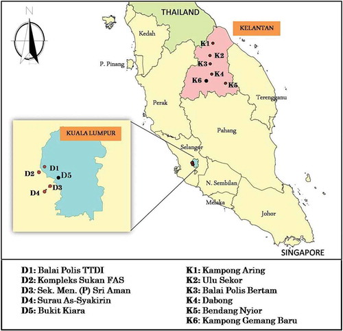
In view of the diverse rainfall profiles and the high variability of rainfall distributions within Peninsular Malaysia, the performance of the STNS (Fo) model is assessed for two regions. The selected regions are the Damansara River basin and the Kelantan River basin. The Damansara River basin (148 km²) is situated within the Klang Valley, which is the most developed and populated area in Malaysia. Unsustainable development and industrialization coupled with convective rains have contributed to the increasing occurrence of flash floods within the basin. In contrast, the Kelantan River basin (13 000 km²) is agriculture-based and located on the northeast of the peninsula. Facing the South China Sea, the region’s rainfall distribution is largely dictated by the monsoon northeast wind. Flooding is a norm during the monsoon season, causing substantial hardship to the residents and damage to properties (Pradhan 2009, Adnan and Atkinson 2011).

The data used in the development of the STNS model consisted of 10 years of hourly and daily rainfall series (1998–2007), taken from several raingauge stations within the vicinity of each basin. Statistical characteristics from the merged data, namely hourly and daily coefficients of variation and autocorrelation function, hourly coefficients of skewness and cross-correlations between sites, are used to develop the STNS model. In the Damansara River basin, observed data are from four stations, Balai Polis TTDI, Kompleks Sukan FAS, Sekolah Menengah (P) Sri Aman and Surau Al-Syakirin. While in the Kelantan River basin, data from five stations, Kampong Aring, Ulu Sekor, Balai Polis Bertam, Dabong and Bendang Nyior, are used as input. Model parameters are determined separately for each basin and, subsequently, Fourier series equations are derived to represent the parameters. To assess the capability of the STNS (Fo) model, simulation processes are conducted at independent locations within the studied regions: Bukit Kiara in the Damansara River basin and Kampong Gemang Baru in the Kelantan River basin. The basins and the locations of the stations used are shown in Figure 1.

Figure 1. Map of Peninsular Malaysia showing stations used in the study.

4 Results and discussion

The estimated parameters of the original STNS model at both basins are shown in Tables 2 and 3. Based on these parameters, hourly rainfall series of 10-year length for every month are generated at the chosen sites and statistical characteristics from the results are derived. Boxplots for each statistical characteristic are constructed. Figures 2 and 3 show boxplots of the simulated series drawn against the observed data for both basins. These results are later compared to the results of the proposed STNS (Fo) model.

Table 2. Estimated parameters of the STNS model for the Damansara River basin.

Jan	0.0086	0.2496	11.2982	4.9995	16.5862	0.5536	0.5511	0.65	4.1466
Feb	0.0119	0.4649	7.5793	5.2177	30.3793	2.5689	7.9602	0.65	7.5948
Mar	0.0100	0.0129	8.8253	3.0171	23.4080	0.3383	0.1607	0.65	5.8520
Apr	0.0076	0.0103	7.9877	2.9997	30.6137	0.3993	0.2027	0.65	7.6534
May	0.0097	0.0633	3.8958	2.7684	27.1671	0.8883	0.4892	0.65	6.7918
June	0.0065	0.2579	12.1824	5.3385	19.4031	1.6511	5.2855	0.65	4.8508
July	0.0095	0.1231	8.6575	4.4629	19.2545	0.4488	0.2775	0.65	4.8136
Aug	0.0100	0.1474	5.2950	3.8466	29.4387	0.6070	0.3106	0.65	7.3597
Sept	0.0100	0.1062	6.4950	3.2082	29.0067	0.4130	0.1763	0.65	7.2517
Oct	0.0100	0.0793	8.2291	3.5953	25.2649	0.3805	0.1896	0.65	6.3162
Nov	0.0089	0.0140	9.9934	2.5348	17.9671	0.3858	0.2367	0.65	4.4918
Dec	0.0096	0.0147	6.4262	2.9998	23.7301	0.4968	0.2524	0.65	5.9325

(Norzaida et al. 2014)

Table 3. Estimated parameters of the STNS model for the Kelantan River basin.

Jan	0.004	0.032	17.9985	1.6164	12.7235	0.1549	0.0687	0.65	0.0943
Feb	0.0022	0.0576	17.999	1.6445	14.4158	0.2001	0.1147	0.65	0.3629
Mar	0.0091	0.0651	7.019	2.3798	17.7634	0.1855	0.0385	0.65	1.5311
Apr	0.013	0.0507	3.4474	2.2809	21.6016	0.1792	0.0176	0.65	1.4853
May	0.0156	0.1184	5.5748	2.351	17.5328	0.1407	0.0176	0.65	2.4975
June	0.0282	0.1352	2.8151	2.6818	21.0232	0.2382	0.0254	0.65	0.3404
July	0.0388	0.0974	2.3412	3.1894	19.4421	0.1229	0.0056	0.65	1.6318
Aug	0.0099	0.0100	7.1293	2.2262	23.1694	0.1395	0.0221	0.65	0.7479
Sept	0.0312	0.1000	3.4601	2.7556	20.3907	0.2015	0.0224	0.65	0.8503
Oct	0.0201	0.0926	6.1679	2.9559	24.0292	0.1749	0.0300	0.65	0.5865
Nov	0.0074	0.0391	14.9622	2.219	20.2648	0.2004	0.0957	0.65	0.0257
Dec	0.0073	0.0342	24.9998	1.1955	12.3197	0.1397	0.0777	0.65	1.0608

Figure 2. Comparison between simulated hourly series (box plots) of STNS model and observed data (line graph) for the Damansara River basin.

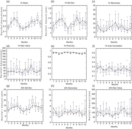
Figure 3. Comparison between simulated hourly series (box plots) of STNS model and observed data (dotted line) for the Kelantan River basin.

The second part of the study is about data simulation in the STNS (Fo) model. Model development and simulation results for each basin are in the following sections.

4.1 Damansara River basin

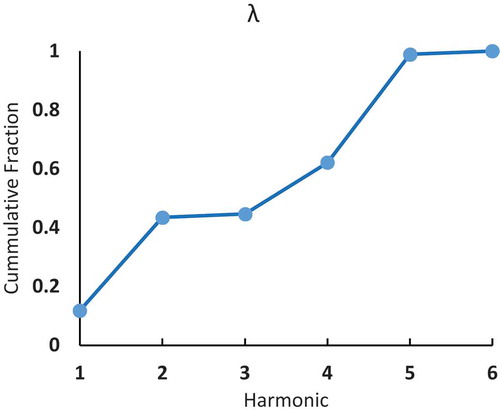
The number of significant harmonics for parameters , , , and is determined by analysing the cumulative fraction of the total variance explained by the harmonics. Based on the selection criteria, the number of harmonics that contribute significantly to the total variance would increase rapidly. The cumulative fraction of total variance given by the first Q harmonics Ŧ of the parameters is shown in Table 4, with the Ŧ that contribute significantly given in bold. For instance, the first five harmonics contribute about 99.01% of the total variance for parameter . Figure 4 shows a graph of Ŧ against the number of harmonics for parameter . Summing up, the significant harmonics for , , , and are 5, 4, 5, 4 and 5, respectively. The findings are consistent with the highly variable rainfall distribution in Malaysia, where a significant harmonic of at least 3 is anticipated.

Table 4. Cumulative fraction of total variance for each parameter for the Damansara River basin.

Harmonic
1	0.1182	0.0337	0.0401	0.0272	0.0375
2	0.4354	0.4159	0.1402	0.5263	0.3975
3	0.4472	0.7724	0.4115	0.7982	0.5075
4	0.6207	0.8277	0.6040	0.8340	0.5759
5	0.9901	0.8751	0.9943	0.8737	0.7000
6	1.0000	1.0000	1.0000	1.0000	1.0000

Figure 4. Cumulative fraction of total variance explained by each harmonic for in the Damansara River basin.

These results are used in equation (2) to determine Fourier series coefficients ( and ) of each parameter (see Table 5). Subsequently, Fourier series equations representing the parameters are formed with these values of and For example, the equations representing parameters and are:

(7)

(8)

Table 5. Fourier coefficients for each parameter of the STNS (Fo) model for the Damansara River basin.

Parameters	Harmonics
λ (lambda)	1	0.0094	0.0006	–0.0805 × 10^−3
	2		–0.0009	0.5485 × 10^−3
	3		–0.0002	–0.0167 × 10^−3
	4		–0.0003	–0.6928 × 10^−3
	5		0.0011	0.0638 × 10^−3
β (beta)	1	0.1286	0.0028	0.0350
	2		0.0046	0.1181
	3		–0.1049	0.0449
	4		–0.0307	–0.0328
(mu C)	1	8.0721	0.5124	0.3952
	2		0.9442	0.3932
	3		–1.3803	–0.9645
	4		0.4101	1.3581
	5		–2.0102	–0.1946
η (eta)	1	3.7490	−0.1822	0.1443
	2		0.2777	0.9567
	3		–0.7176	0.1602
	4		–0.1081	0.2439
θ (theta)	1	24.3516	−1.3592	0.5190
	2		–4.4404	–0.7728
	3		1.4559	2.0217
	4		–0.4646	–1.9100
	5		2.0669	–1.2966

Once Fourier series equations of the parameters have been identified, hourly rainfall series for a 10-year period are simulated for Bukit Kiara. Statistical characteristics based on the simulated data are derived and a boxplot is created for each statistic. Figure 5 shows boxplots of simulated series constructed against observed statistics.

Figure 5. Comparison between simulated hourly series (box plots) of STNS (Fo) model and observed data (dotted lines) for the Damansara River basin.

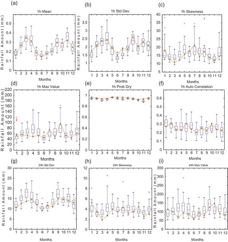
The STNS (Fo) model performs rather well, with the simulated rainfall series in agreement with the observed data. The hourly mean and standard deviation (Fig. 5(a) and (b)) match excellently with the observed data. The generated hourly mean coincides well with the bimodal pattern observed during the inter-monsoon seasons. During these periods, the basin experienced high rainfall brought by short storms. Standard deviations were also high during the said seasons, reflecting large variations of rainfall intensity. The hourly maximum values (Fig. 5(d)) were adequately represented. The chart shows that the maximum values of observed data did not follow the bimodal pattern of the inter-monsoon season, while the data generated from the model are more consistent with the pattern. This corresponds with the study by Zalina et al. (2007), which described the period of 2000–2006, and showed that the maximum values of observed rainfall in Malaysia were no longer reserved for the inter-monsoon months. Hence, the results produced are quite satisfactory considering that the maximum values of historical data were not included in the model formation.

Figure 5(c) shows that the skewness of the observed rainfall distribution within the basin is quite high, echoing the high variability of convective rains. A bimodal pattern is detected with relatively low skewness recorded during the inter-monsoon seasons. The chart reveals that the STNS (Fo) model is able to capture the skewness trend quite well.

Other statistical characteristics at the hourly scale, such as autocorrelation coefficient and probability of dry period, and at the daily scale, the standard deviation, skewness and maximum values, compare reasonably well with the observed data.

4.2 Kelantan River basin

Model development and assessment within the basin is identical to the study in the Damansara River basin. Significant harmonics (Table 6) , , , and are 6, 5, 6, 5 and 5, respectively, and the Fourier series coefficients and for the parameters are given in Table 7.

Table 6. Cumulative fraction of total variance for the parameters for the Kelantan River basin.

Harmonic
1	0.5715	0.3104	0.71 645	0.56 645	0.4762
2	0.5746	0.4019	0.8704	0.6613	0.7222
3	0.6177	0.7603	0.8915	0.8161	0.7695
4	0.7823	0.8440	0.9397	0.8305	0.7970
5	0.8294	0.9081	0.9435	0.9105	0.8762
6	0.9336	0.9458	0.9862	0.9999	0.9308
7	1.0000	1.0000	1.0000	1.0000	1.0000

Table 7. Fourier coefficients for parameters of the STNS (Fo) model for the Kelantan River basin.

Parameters	Harmonics
λ	1	0.0156	−0.0097	−0.0080
	2		0.0009	–0.0002
	3		–0.0034	–0.0007
	4		0.0034	0.0059
	5		0.0027	–0.0038
	6		–0.0042	–0.0000
β	1	0.0694	−0.0303	−0.0038
	2		0.0071	–0.0150
	3		–0.0317	0.0081
	4		0.0143	0.0069
	5		0.0115	–0.0055
	1	9.4929	8.4449	2.2919
	2		3.4004	2.2106
	3		1.4324	0.4518
	4		0.0806	–2.2676
	5		1.2151	–0.0606
	6		1.8671	–0.0000
η	1	2.2913	−0.4860	−0.3641
	2		–0.1873	–0.1631
	3		–0.2633	–0.1775
	4		–0.0382	0.2312
	5		0.0062	–0.0013
θ	1	18.7230	−2.5532	−2.8393
	2		–1.9063	–1.9742
	3		–0.3962	–1.1372
	4		–0.8488	0.3484
	5		–1.4023	0.3884

As before, Fourier series equations are formed based on these significant harmonics and coefficients , and . For instance, Equation (9) is the Fourier series equation representing parameter . The rest of the equations could easily be formed by using Table 7.

(9)

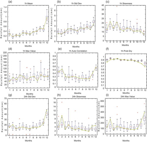
Simulation of hourly rainfall series is conducted for Kampong Gemang Baru. Statistical characteristics are derived from the simulation results and boxplots are constructed. Comparison of these boxplots and observed data are presented in Figure 6. It can be seen that the STNS (Fo) model is able to generate rainfall series comparable to the observed data.

Figure 6. Comparison between simulated hourly series (box plots) of STNS (Fo) model and observed data (line graph) for the Kelantan River basin.

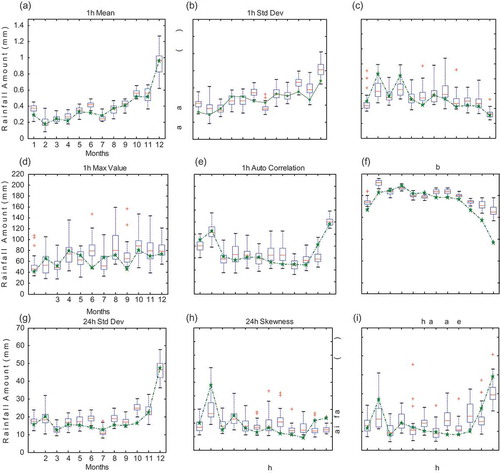
The hourly mean (Fig. 6(a)) matches excellently with the observed data. The generated data are able to imitate the distinct pattern exhibited during the northeast monsoon season. Unlike the distribution of convective rains, monsoon rains exhibit a unimodal pattern which usually peaks during the month of December. Most of the monsoon flood incidences occurred during this period. A prominent trait of the monsoon rains is the relatively low intensity but long duration, which can be several days. This trait is reflected in the observed hourly maximum value (Fig. 6(d)) and daily maximum value (Fig. 6(i)). Notice that the observed daily maximums exhibit the typical pattern, hitting the highest point in December, while the hourly maximums do not portray a particular pattern. Hence, the model has produced reasonable hourly and daily maximum estimates throughout the year, especially during the monsoon season. Such estimates are satisfactory since maximum values of rainfall in Kelantan are highly variable due to the large influence of monsoon winds coming from the South China Sea.

Other statistical characteristics at the hourly scale, such as standard deviation, coefficient of skewness, autocorrelation and maximum values, match excellently to reasonably well with observed data. The same is also true for the daily scale. The standard deviation, coefficient of skewness, autocorrelation and maximum values of the generated series are comparable to the actual data. However, the model has a tendency to overestimate the probability of a dry period at the hourly scale.

4.3 Comparing the performance of STNS and STNS (Fo) models

The performance of both STNS and STNS (Fo) models is quite similar in preserving the statistical characteristics of rainfall for both basins (Figs 2, 3, 5 and 6). RMSE tests are employed to compare the models’ ability to match observed data. Tables 8 and 9 summarize the RMSE for each model at both sites, with the lowest RMSE value given in bold. Results show that the original STNS model performs slightly better than STNS (Fo) in both basins. In the Damansara River basin, the latter model is better at mean, coefficient of skewness and maximum values at the hourly scale, with standard deviation and maximum values better at the daily scale. In the Kelantan River basin, the STNS model performs better for all the statistical characteristics at the hourly scale and standard deviation at the daily scale. Although the STNS model appears to be better for both basins, the differences between simulation results are marginal. On the whole, STNS (Fo) performs adequately, particularly at the hourly scale in the Damansara River basin, and at the daily scale in the Kelantan River basin.

Table 8. The RMSE for the STNS models for the Damansara River basin.

	STNS	STNS (Fo)
1 h mean	0.01 656	0.01 858
1 h std dev	0.21 041	0.17 242
1 h coefficient of skewness	2.52 140	2.55 734
1 h max value	13.79 166	14.34 655
1 h prob dry	0.02 417	0.02 148
1 h autocorrelation	0.08 449	0.03 498
24 h std dev	1.40 329	1.96 414
24 h coefficient of skewness	0.92 970	0.97 097
24 h max value	24.98 788	30.30 180

Table 9. The RMSE for the STNS models for the Kelantan River basin.

	STNS	STNS (Fo)
1 h mean	0.022 292	0.046 545
1 h std dev	0.300 518	0.406 925
1 h skewness	2.08 716	2.422 534
1 h max value	10.20 032	13.2796
1 h prob dry	0.050 271	0.051 064
1 h autocorrelation	0.040 491	0.182 697
24 h std dev	3.13 015	3.312 407
24 h skewness	1.565 521	1.552 986
24 h max value	59.53 208	57.9506

4.4 Validation of the STNS (Fo) model

The study further conducted a 2-year data simulation at both basins to validate the models. The results are summarized in the form of boxplots and compared to historical data for 2008/09 (see Figs 7 and 8). Simulated results indicate that the model is able to preserve fairly well the statistical characteristics of observed data at both basins. In the Damansara River basin, the generated data resemble the observed data reasonably well, except for the hourly probability of a dry period, which the model has a tendency to overestimate for the whole 12 months. The result is quite unexpected, since the probability of a dry period at the hourly scale is well represented during the calibration period. The overall results for the Kelantan River basin show that the model fairly well preserves the statistical characteristics of observed data. Similarly, the hourly probability of a dry period also tends to be overestimated, especially during the northeast monsoon season. However, for both basins the model is able to adequately predict the maximum value at hourly and daily scales, although such characteristics are not included in the model formation.

Figure 7. Comparison between simulated hourly series (box plots) of STNS (Fo) model and observed data (dotted line) for the Damansara River basin for validation period.

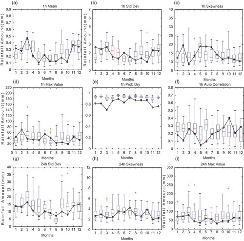
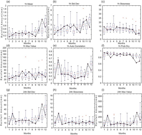
Figure 8. Comparison between simulated hourly series (box plots) of STNS (Fo) model and observed data (line graph) for the Kelantan River basin for validation period.

On the whole, the validation results are well regarded considering there are some discrepancies between the historical data for the calibration period (1998–2007) and the validation period (2008/09). This is supported by studies by Syafrina et al. (2014b) and Norzaida (2012), which indicated that there is an increasing trend of annual rainfall during the period of study.

5 Conclusions

Rainfall data at high resolution are very much needed in studies concerning flooding. Especially in tropical regions where rainfall is highly variable, the task of generating credible data at a fine time scale, such as hourly, is very challenging. This study is designed to assess the feasibility of using Fourier series to describe the seasonal variations of the rainfall process by representing the model’s parameters throughout the year. Instead of having the parameters constant for each month, the parameters are assumed to change continuously with time over the year. Consequently, the rainfall model should be more parsimonious with a reduced number of parameters.

The proposed technique is applied to Malaysia’s tropical rainfall, which is known to be very variable in time and space. The model is assessed for two regions within Peninsular Malaysia with contrasting rainfall profiles: an urban area having convective rain and a non-urban area having monsoonal rain. Data simulations are conducted for independent locations. In addition, model formation does not include data such as maximum value of rainfall and probability of dry period. A comparative study between the original STNS and the proposed STNS (Fo) model is conducted to evaluate the models’ performance. Model validation is also conducted to measure the models’ predictive ability.

The formation of STNS (Fo) models for both basins reveals that the number of significant harmonics that represent parameters’ yearly oscillations is found to be slightly lower for convective rain compared to monsoonal rain. Results of model applications in both basins indicated that the STNS (Fo) model is able to generate rainfall series that match the observed data. The model, however, performed better for the Damansara River basin. A possible explanation for this might be that the Damansara River basin is much smaller in size, thus the estimated parameters are much more precise. Another possibility is that the “strength” of the northeast monsoon wind that brings rain to the Kelantan River basin is unpredictable from year to year. Basically, the wind stems from the monsoon surges or tropical depressions formed in the South China Sea due to the outburst of cold air from Siberia. In addition, work by Suhaila et al. (2010) showed there have been significant increases in rainfall intensity and extreme occurrence during the northeast monsoon. It is also observed that both the original STNS model and the STNS (Fo) model have a tendency to overestimate the hourly probability of a dry period for monsoonal rainfall. This issue needs further investigation in order to improve both models.

Model validation for both river basins indicates that the STNS (Fo) model is able to make commendable predictions of hourly rainfall series. The generated series preserve most of the statistical characteristics, but there are some limitations in the representation of probability of a dry period at the hourly scale. However, the maximum values at hourly and daily scales, although excluded from the parameter estimation process, are reasonably preserved by the model.

On the whole, comparisons using RMSE reveal that the performance of the original STNS and STNS (Fo) models at both basins is quite similar. The inclusion of Fourier series to represent the yearly seasonality managed to produce equivalent results despite having fewer parameters. Considering there are only slight differences, the STNS (Fo) model is a better option as it is much more parsimonious. It can be concluded that the proposed STNS (Fo) model is capable of generating tropical rainfall series from convective and monsoonal activities.

Acknowledgements

The authors thank the Department of Irrigation and Drainage Malaysia for providing the required data and acknowledge the support and cooperation given by the Research Management Unit of Universiti Teknologi Malaysia. Constructive recommendations by reviewers are also gratefully acknowledged.

Disclosure statement

No potential conflict of interest was reported by the authors.

Additional information

Funding

This study is funded by the Ministry of Higher Education Malaysia under GUP Vote 09H08.

References

- Adnan, N.A. and Atkinson, P.M., 2011. Exploring the impact of climate and land use changes on streamflow trends in a monsoon catchment. International Journal of Climatology, 31, 815–831. doi:10.1002/joc.v31.6
- Bayazit, M., Onoz, B., and Aksoy, H., 2001. Nonparametric streamflow simulation by wavelet of Fourier analysis. Hydrological Sciences Journal, 46, 623–634. doi:10.1080/02626660109492855
- Burlando, P. and Rosso, R., 1993. Stochastic models of temporal rainfall: reproducibility, estimation and prediction of extreme events. In: J.D. Salas, R. Harboe, and J. Marco-Segura, eds. Stochastic hydrology in its use in water resources systems simulation and optimization. Dordrecht: Kluwer Academic Pub, 137–173.
- Calenda, G. and Napolitano, F., 1999. Parameter estimation of Neyman-Scott processes for temporal point rainfall simulation. Journal of Hydrology, 225, 45–66. doi:10.1016/S0022-1694(99)00133-X
- Cowpertwait, P., 1998. A Poisson-cluster model of rainfall: high order moments and extreme values. Proceedings of the Royal Society of London. Series A, 454, 885–898. doi:10.1098/rspa.1998.0191
- Cowpertwait, P., 2006. A spatial–temporal point process model of rainfall for the Thames catchment, UK. Journal of Hydrology, 330, 586–595. doi:10.1016/j.jhydrol.2006.04.043
- Cowpertwait, P.S.P., 1991. Further developments of the Neyman–Scott clustered point process for modelling rainfall. Water Resources Research, 27, 1431–1438. doi:10.1029/91WR00479
- Cowpertwait, P.S.P., 1995. A generalized spatial–temporal model of rainfall based on a clustered point process. Proceedings of the Royal Society of London, Series A: Mathematics and Physical Sciences, 450, 163–175. doi:10.1098/rspa.1995.0077
- Cowpertwait, P.S.P. and Kilsby, C.G., 2002. A space-time Neyman-Scott model of rainfall: empirical analysis of extremes. Water Resources Research, 38, 6-1–6-14. doi:10.1029/2001WR000709
- Davis, J.C., 1986. Statistics and data analysis in geology. 2nd ed. New York: J. Wiley and Sons.
- Duan, Q., Sorooshian, S., and Gupta, V., 1992. Effective and efficient global optimization for conceptual rainfall-runoff models. Water Resources Research, 28 (4), 1015–1031. doi:10.1029/91WR02985
- Fadhilah, Y., et al., 2007. Fitting the best fit distribution for the hourly rainfall amount in the Wilayah Persekutuan. Journal Teknologi UTM, 46 (C), 49–58.
- Fadhilah, Y., 2008. Stochastic modelling of hourly rainfall processes. Thesis (Phd). Universiti Teknologi Malaysia.
- Fadhilah, Y., Norzaida, A., and Zalina Mohd, D., 2008. Fourier series in a Neyman Scott rectangular pulse model. Matematika, 24 (2), 237–251.
- Fitzpatrick, E.A., 1964. Seasonal distribution of rainfall in Australia analysed by Fourier methods. Archiv Meteorologie, Geophysik und Bioklimatologie Ser. B., 13 (2), 270–286. doi:10.1007/BF02243257
- Guenni, L., et al., 1996. A model for seasonal variation of rainfall at Adelaide and Turen. Ecological Modelling, 85, 203–217. doi:10.1016/0304-3800(94)00189-8
- Han, S.-Y., 2001. Stochastic modeling of rainfall processes: a comparative study using data from different climatic conditions. Thesis (Masters). McGill University, QC.
- Hutchinson, M.F., 1991. Climatic analyses in data sparse regions. In: R.C. Muchow and J.A. Bellamy, eds. Climatic risk in crop production. Wallingford, U.K.: CAB International, 55–71.
- Islam, S., et al., 1990. Parameter estimation and sensitivity analysis for the modified Bartlett-Lewis rectangular pulses model of rainfall. Journal of Geophysical Research, 95 (D3), 2093–2100.
- Kirkyla, K.I. and Hameed, S., 1989. Harmonic analysis of the seasonal cycle in precipitation over the United States: a comparison between observations and a general circulation model. Journal of Climate, 2, 1463–1475. doi:10.1175/1520-0442(1989)002<1463:HAOTSC>2.0.CO;2
- Kottegoda, N.T., 1980. Stochastic water resources technology. London: Macmillan.
- Leonard, M., et al., 2007. Implementing a space-time rainfall model for the Sydney region. Water Science & Technology, 55, 39–47.
- Machiwal, D. and Jha, M.K., 2008. Comparative evaluation of statistical tests for time series analysis: application to hydrological time series. Hydrological Sciences Journal, 53 (2), 353–366. doi:10.1623/hysj.53.2.353
- Norzaida, A., 2012, Spatial temporal modelling of rainfall process in Malaysia. Thesis (Phd). Universiti Teknologi Malaysia.
- Norzaida, A, Zalina M. D. and Daud, F.Y., 2014. A comparative study of mixed exponential and Weibull distributions in a stochastic model replicating a tropical rainfall process. Theoretical Applied Climatology, 118 (3), 597–607. doi:10.1007/s00704-013-1060-4
- Onof, C. and Wheater, H.S., 1993. Modeling of British Rainfall using a random parameter Bartlett-Lewis rectangular pulse. Journal of Hydrology, 149, 67–95. doi:10.1016/0022-1694(93)90100-N
- Pradhan, B., 2009. Flood susceptible mapping and risk area delineation using logistic regression, GIS and remote sensing. Journal of Spatial Hydrology, 9, 2.
- Rodriguez-Iturbe, I., Cox, D.R., and Isham, V., 1987. Some models for rainfall based on stochastic point processes. Proceeding of the Royal Society of London Series A, 410 (1839), 269–288. doi:10.1098/rspa.1987.0039
- Sabbagh, M.A. and Bryson, R.A., 1962. Aspects of the precipitation climatology of Canada investigated by the method of harmonic analysis. Annals of the Association of American Geographers, 52, 426–440. doi:10.1111/j.1467-8306.1962.tb00423.x
- Salas, J.D., et al., 1980. Applied modelling of hydrologic series. Littleton, CO: Water Resources Publications.
- Stern, R.D. and Coe, R., 1984. A model fitting analysis of daily rainfall data (with discussion). Journal of the Royal Statistical Society. Series A, 147, 1–34.
- Suhaila, J., et al., 2010. Trends in Peninsular Malaysia rainfall data during southwest monsoon and northeast monsoon seasons: 1975–2004. Sains Malaysiana, 39 (4), 533–542.
- Syafrina, A.H., Zalina, M.D., and Juneng, L., 2014a. Future projections of extreme precipitation using Advanced Weather Generator (AWE-GEN) over Peninsular Malaysia. IAHS Red Book, 364, 106–111.
- Syafrina, A.H., Zalina, M.D., and Juneng, L., 2014b. Historical trend of hourly extreme rainfall in Peninsular Malaysia. Theoretical Applied Climatology. doi:0.1007/s00704-014-1145-8
- Woolhiser, D.A. and Pegram, G.G.S., 1979. Maximum likelihood estimation of Fourier coefficients to describe seasonal variations of parameters in stochastic daily precipitation models. Journal of Applied Meteorology, 18, 34–42. doi:10.1175/1520-0450(1979)018<0034:MLEOFC>2.0.CO;2
- Woolhiser, D.A. and Roldán, J., 1986. Seasonal and regional variability of parameters for stochastic daily precipitation models: South Dakota, U.S.A. Water Resources Research, 22, 965–978. doi:10.1029/WR022i006p00965
- Zalina, M.D., et al., 2007. Exploring the anomalies of rainfall events in the Klang Valley. In: National conference world water day 2007, 15–16 April 2007, Terengganu.