Assessment of radar-based locally varying anisotropy on daily rainfall interpolation

ABSTRACT

Spatial variability of rainfall has been recognised as an important factor controlling the hydrological response of catchments. However, gauged daily rainfall data are often available at scattered locations over the catchments. This paper looks into how to capitalise on the spatial structure of radar rainfall data for improving kriging interpolation of limited gauge data over catchments at the 1-km² grid scale, using for the case study 117 gauged stations within the 128 km × 128 km region of the Mt Stapylton weather radar field (near Brisbane, Australia). Correlograms were developed using a Fast Fourier Transform method on the Gaussianised radar and gauged data. It is observed that the correlograms vary from day to day and display significant anisotropy. For the radar data, locally varying anisotropy (LVA) was examined by developing the correlogram centred on each pixel and for different radial distances. Cross-validation was carried out using the empirical correlogram tables, as well as different fitting strategies of a two-dimensional exponential distribution for both the gauged and the radar data. The results indicate that the correlograms based on the radar data outperform the gauged ones as judged by statistical measures including root mean square error, mean bias, mean absolute bias, mean standard deviation and mean inter-quartile range. While the radar data display significant LVA, it was observed that LVA did not significantly improve the estimates compared with the global anisotropy. This was also confirmed by conditional simulation of 120 rainfields using different options of correlogram development.

EDITOR M.C. Acreman; ASSOCIATE EDITOR Q. Zhang

KEYWORDS:

• spatial rainfall
• radar
• correlogram
• interpolation
• anisotropy
• cross-validation

1 Introduction

Grid-based spatially-distributed hydrological modelling has become a common practice largely due to advances in computer technology and availability of geographic information systems. However, the basic input of daily rainfall is not available at the desired grid spacing (e.g. 1 km × 1 km) with global gauge densities varying from 1 per 25 km² to over 10 000 km². Availability of daily rainfall data at the desired grid spacing, and record length, enhances the capabilities of hydrological models including those used for water balance studies, sediment yield, sensitivity analysis of reservoirs, soil moisture accounting for irrigation purposes and assessment of climate change.

The problem of generating continuous spatial daily rainfall fields, starting from irregularly distributed daily raingauge data that this paper addresses, falls into the general class of spatial interpolation. Spatial interpolation techniques abound in the literature, highlighting the importance of the topic. Nearly all of the techniques share the general estimation formula of weighted average of the sampled data and the differences are basically how the weights are calculated. Some notable interpolation techniques of deterministic nature applied to rainfall include nearest neighbours (Isaaks and Srivastava 1990), thin plate splines (Jeffrey et al. 2001), inverse weighted distance (Teegavarapu and Chandramouli 2005) and of stochastic nature include kriging (Ly et al. 2011) and spatial copula (Bárdossy and Pegram, 2009). Some variants of the techniques incorporate covariates such as elevation to improve the estimates (Goovaerts 2000).

Ground-based meteorological radar rainfall data have recently been employed to improve infilling or interpolation of gauged rainfall data. While radar helps to improve our understanding of the temporal and spatial structure of rainfall, associated problems leading to either underestimation or overestimation are well recognised (Austin 1987, Krajewski et al. 2010). The sources of errors include existence of clutter and the methods used for conversion of radar reflectivity to rainfall intensity. Therefore, the direct use of radar data in water resources as carried out by Quirmbach and Schultz (2002) has been limited. Rather, some attempts have been made to adjust the radar data using limited gauged data by techniques such as mean bias reduction and error variance minimisation (Wang et al. 2013, Rabiei and Haberlandt 2015). The most popular means of incorporating the radar data is by using them as secondary information in various forms of kriging. In ordinary kriging (co-kriging), the radar data are used to develop the required correlogram, the spatial structure (Krajewski 1987, Gyasi-Agyei and Pegram 2014), while in the case of kriging with external drift the correlogram is developed from the residual of the linear fit of the gauged and collocated radar data, and sometimes with additional information such as topography (Verworn and Haberlandt 2011). Velasco-Forero et al. (2009) evaluated three methods of incorporating the radar information to estimate rainfall fields and concluded kriging with external drift was the preferred option. Conditional merging (Sinclair and Pegram 2005, Ehret et al. 2008) is one of the techniques to combine radar and raingauge data for generation of rainfields. It involves superposition of rainfall variability information obtained from radar data by unconditional simulation on kriged surfaces of observed raingauge data.

Satellite-based high-resolution rainfall products (e.g. CMORTH, TMPA 3B42, TMPA 3B42RT, and PERSIANN) are other sources of data for regions with limited or without ground-based radar and gauges. These data sources also have problems with accuracy due to atmospheric effects and gaps in revisit times among others, and the spatial scales are much coarser than ground-based radar observations. Bitew and Gebremichael (2011) evaluated these products through streamflow simulation with the SWAT hydrological model on a daily timescale and observed that the results were significantly different.

Many of the studies in the literature condition the radar information on the observed gauged data for use at the same region. This paper follows the approach presented by Gyasi-Agyei and Pegram (2014) where attempts were made to understand the spatial structure of the radar data for possible transfer of information from the rich to the poor areas (data-wise) for maximum benefit in terms of uncertainty. For this reason kriging with External Drift may not be appropriate. As noted by Gyasi-Agyei and Pegram (2014), the 6-min radar scans used to extract the spatial dependence of the daily accumulations were not bias corrected, the main reason being that they are not directly used in the interpolation exercise. Bias correction involving shifting and scaling would not affect the spatial correlation structure because the correlations between raw and standardised variables are technically identical.

A major difference between this paper and Gyasi-Agyei and Pegram (2014) is the detailed analysis of radar data to explore the possibility of incorporating locally varying anisotropy (LVA). The methodology involves transforming the daily data to normal scores with which all computations are carried out, and this procedure is first presented. Different options for developing correlograms from the gauged and the radar data, and the fitting of a two-dimensional (2D) exponential distribution, are next described. A brief overview of ordinary kriging and the cross-validation strategies follow. This section is followed by the results and discussions in the penultimate section before the conclusions.

2 Methods

This section begins with the description of the study area and data, and the associated transformation to the normal score using empirical distribution function. All procedures used in the paper are presented under this section.

2.1 Study area and data

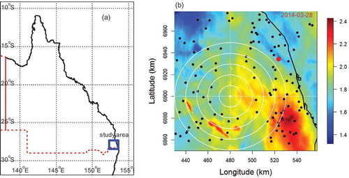
For reasons of Fast Fourier Transform (FFT) analysis explained later, a 128 km × 128 km region within the range of the Mt. Stapylton weather radar station near Brisbane, Queensland (Fig. 1) was selected for this study. This region experiences a subtropical climate (average temperature of 26.5°C) but with hot humid summers (December–February) and moderately dry winters (June–August). Thunderstorms with torrential rain are common. The mean annual rainfall is about 990 mm with an average of 124 wet days per year. The Mt Stapylton radar is a 1500 S-band Doppler type located at latitude 27.718°S and longitude 153.240°E, shown as a red dot in Fig. 1(b). The R spTransform function with the datum set to WGS84 for zone 56 was used to convert the longitude and latitude coordinate system to the Universal Transverse Mercator (UTM) Eastings and Northings coordinate system to conform to the radar data grid resolution of 1 km². Within the study area there are 117 daily rainfall gauges (locations shown as black dots in Fig. 1(b), translating to a gauge density of 1 per 140 km² and an average interstation distance of nearly 12 km. However, a few gauges malfunctioned for some wet days and were omitted from the analysis.

Figure 1. Location of (a) the study area in Queensland, Australia, and (b) the 117 daily gauge stations (black dots) within the range of the Mt. Stapylton weather radar station (near Brisbane) (red dot); the radar image in log10(mm) scale is for 28-03-2014.

Four months’ (January–April 2014) radar data and the corresponding daily rainfall data were obtained from the Australian Bureau of Meteorology. The 6-min volume scans of the radar data were aggregated over the 24-hour day ending at 09:00 to conform with the daily rainfall sampling timescale. Table 1 shows 12 wet days (events) having different properties selected for examination. The statistics were compiled for the gauged, collocated (radar data at gauged locations) and the full radar data. The wetted area ratio, defined as the number of wet days (pixels or nodes used interchangeably) divided by the total number of gauges (pixels), could be different for these data sets of the same day. This is also true for the maximum wet gauge/pixel amount. However, the average wet gauge amount, defined as the sum of all rainfall data divided by the number of wet gauges/pixels, shows close similarity between the collocated and the full radar values. Therefore, there is a high potential to use this latter statistical measure to screen simulated rainfields.

Table 1. Basic properties of selected wet days.

Date	Number of gauges	Wetted area ratio			Average wet gauge amount (mm)			Maximum wet gauge amount (mm)			Gauge–collocated correlation
		Gauge	Collocated	Radar	Gauge	Collocated	Radar	Gauge	Collocated	Radar
14 January 2014	109	0.450	0.248	0.191	3.2	2.5	2.3	7.4	6.7	11.1	0.57
20 February 2014	109	0.184	0.184	0.166	15.0	6.0	5.9	31.4	15.2	23.5	0.92
24 February 2014	102	0.578	0.402	0.311	4.4	4.5	4.2	15.0	18.4	21.6	0.70
25 February 2014	111	0.568	0.297	0.240	4.8	3.9	3.9	17.4	11.4	19.5	0.66
05 March 2014	109	0.560	0.367	0.284	6.9	4.6	6.4	24.2	17.2	45.4	0.78
09 March 2014	104	0.356	0.481	0.439	2.9	3.5	3.0	6.6	10.9	16.6	0.62
10 March 2014	98	0.786	0.510	0.391	5.7	3.6	3.5	22.1	13.2	17.6	0.63
25 March 2014	107	0.935	1.000	0.996	19.5	22.8	24.5	110.2	82.3	168.3	0.79
26 March 2014	107	0.991	1.000	1.000	24.1	24.4	21.7	58.0	59.8	99.2	0.72
27 March 2014	108	0.954	1.000	1.000	11.3	37.0	36.8	37.2	130.3	160.8	0.21
28 March 2014	109	1.000	1.000	1.000	133.9	87.1	77.6	319.4	233.6	266.5	0.83
14 April 2014	94	0.830	0.436	0.512	6.6	3.7	3.5	30.2	22.0	27.4	0.65

The daily rainfall data were treated independently and quantile-quantile (Q-Q) transformation was applied to obtain normal scores. This transformation was considered as appropriate since ordinary kriging implicitly assumes normality of the data, and also the multivariate normal distribution has a unique advantage being that the second order moments are sufficient. The process involves the use of an empirical marginal distribution to convert the daily rainfall values, Z(j), in mm, at gauge locations (j) into the uniform domain and then convert the uniform domain into standard normal quantiles as:

(1)

where Φ is the cumulative normal distribution N(0,1) and F{Z(j)} is the empirical distribution defined as the ratio of the increasing order of magnitude rank to the number of stations plus one. The zeros (values less than 1 mm, the minimum wet gauge value) in the daily rainfall data were censored as varying uniformly (U) between w_m = Φ^-1[1/(N + 1)] and the Rosenblueth (1975) mean w₀ =—ϕ[Φ-1(p₀)]/p₀, where ϕ is the standard normal density function and p₀ is the dry probability defined as the number of dry gauges over the total number of gauges (N). In Gyasi-Agyei and Pegram (2014), w₀ was set for all zeros but it has been observed that the ordinary kriging equations may become unstable for days with a considerable number of dry gauges. Sampling from the uniform distribution avoided this numerical instability problem, and also the dry gauges were kept apart from the wet gauges. There is a possibility of the quantiles of the simulated random field exceeding the observed gauged values. Most extreme value distributions tending to the exponential, the empirical distribution is extrapolated using an exponential distribution fitted to the two unique largest observed values as:

(2)

where z_e and p_e are the second largest station rainfall value and the corresponding relative frequency, respectively. The largest station rainfall amount and the corresponding relative frequency were used to estimate the exponential parameter L. The methodology for determining the spatial correlograms is next presented. Note that, because the kriging is carried in the standard normal scores domain, the field variance is unity and, as such, the correlogram is the same as the covariogram required by the kriging equations.

2.2 Estimation of the spatial correlogram

A considerable amount of correlogram development is required, so an automated procedure was preferred. The automated method of developing the covariance of the spatial structure presented by Yao and Journel (1998) was adopted. It is based on Bochner’s theorem that achieves a positive definite covariance lookup table through “round-trip” FFT with intermediate smoothing processes. Application of FFT requires that the dimension of the study region be a power of two to speed up the computations, hence the 128 km × 128 km study region. Three steps are involved in the estimation of the correlogram:

• Step 1: Calculation of the sample covariance map using the normal score of the scattered gauged rainfall or the gridded radar data as:

  (3)

where w(s_k) is a standardised Gaussianised daily rainfall value of gauge k located at s_k; h is the lag distance and has components (h_i, h_j) in the i (x) and j (y) directions, respectively; N_h is the number of contributing gauge pairs at lag h (km), m_w-h and m_w+h are the mean of the pair tail and head values, and the empirical correlogram values. Infilling of the uninformed or poorly informed entries is carried out by interpolation, necessary particularly for the scattered gauged data.

• Step 2: Smoothing of the large fluctuations and missing entries that might be present after step 1. Each entry is replaced with a weighted average within a radial moving window.

• Step 3: The gridded sample covariance map is transformed to a quasi-density spectrum map in the frequency domain by FFT. Here too a moving window is used to smooth the spectrum map under the constraint of positivity and unit sum. The smoothed spectrum map is then inverse FFT to obtain the required correlogram lookup table which is positive definite and with all sample fluctuations, in particular for the scattered data, filtered out.

Velasco-Forero et al. (2009) used this approach to model anisotropic variograms of 1-hour radar accumulations. We have gone a step further to model the shape of the correlogram using a 2D exponential model and also investigated the effects of the locally varying anisotropy exhibited by the radar rainfields.

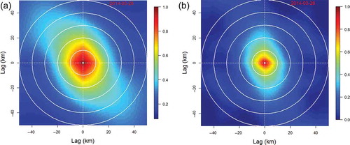
Figure 1(b) shows the rainfall radar image in log10(mm) scale for 28 March 2014, the wettest day for the period under consideration. In Fig. 2, the empirical correlogram maps developed using both the radar (Fig. 2(a)) and gauged (Fig. 2(b)) data are shown. Anisotropy is clearly displayed in both correlograms and the parameters could vary depending on the lag (distance between a pair of gauges). The range and anisotropy ratio seem to be increasing with distance from the correlogram centre. It needs to be noted that the anisotropy parameters (range and ratio) and the direction could be different for the gauged and radar data for the same day.

Figure 2. (a) Radar data empirical correlogram and (b) correlogram of the gauged data for 28-03-2014. Concentric circles encompass areas within {10, 20, 30, 40, 50} km radius from the correlogram map centre.

The observed elliptical contours of the correlogram are modelled by a 2D exponential distribution, R_Θ(x,y)= R_Θ(u,v), of the form:

(4)

where u is the lag distance along the major axis of the elliptical contour making an angle of θ (between 0 and 180) degrees measured anticlockwise from the +X (east) direction. Similarly, distance v along the minor axis makes the same angle with the +Y axis. Parameter L_u is the correlation length of the major axis and η is the anisotropy ratio (ratio of minor to major axis correlation lengths). Parameter a_n is the sill (between 0 and 1) and the nugget is (1 – a_n). The four parameters were estimated using the global optimisation technique of Duan et al. (1992) subject to the objective function:

(5)

where h_i,j is the distance of grid cell (i,j) from the centre of the sample correlogram map.

In order to understand the effects of the observed anisotropy on the kriging of scattered observed rainfall data, the following options for developing the 2D exponential parameters were proposed. For the regional options (gauge and radar) all data were used while the LVA options were restricted to the radar data and local values within a set radius.

Regional options were developed as:

• REG_0: the empirical correlogram map (lookup table) using all data;

• REG_1: one parameter set estimated for the correlogram map in REG_0;

• REG_2: as in REG_1 with the exception that parameter sets were developed using correlogram values within each of the concentric circles with radii of {10, 20, 30, 40, 50 km} as shown in Fig. 2; during kriging, the particular parameter set used was determined by the average of the distances between the neighbouring points and the target point; e.g. if the average distance was 11 km then the parameter set defined by the 20 km radius was used;

• REG_3: similar to REG_2 with the exception that the correlogram values between the concentric circles were used to estimate the parameter sets instead of all values within the circle.

For the locally varying anisotropy (LVA) options, and for each target location, radar rainfall pixel values within a set radius of {10, 20, 30, 40, 50 km} as shown in Fig. 1(b) were used to develop the correlogram map and fitted as in REG_1. Therefore, for each pixel there were five parameter sets:

• LVA_0: the average distance between each target location and the neighbours was used to select the required parameter set; therefore, a mixture of the five radii parameter sets were used;

• LVA_1: same as LVA_0 but using local 10 km radius parameter sets only;

• LVA_2: same as LVA_0 but using local 20 km radius parameter sets only;

• LVA_3: same as LVA_0 but using local 30 km radius parameter sets only;

• LVA_4: same as LVA_0 but using local 40 km radius parameter sets only;

• LVA_5: same as LVA_0 but using local 50 km radius parameter sets only.

In order to limit computational time, parameter sets at 5 km centres of the radar image were first estimated. This was followed by inverse weighted distance interpolation over the 1 km × 1 km grid without undue loss of accuracy. For the anisotropy direction, each 5-km centre value was resolved into the horizontal and vertical axes. The vertical and horizontal components were each interpolated over the 1-km² grid and the direction for the fine grid was determined as the inverse tan of the vertical/horizontal components.

2.3 Ordinary kriging and random rainfields generation

Ordinary kriging has been used in many fields for interpolating point measurements over a regular grid, or for infilling (e.g. Cressie 1993) for many years and the mathematics is well established in the literature. Essentially, it is a linear weighted least squares estimate of the w(s₀) variable at the target location s₀ using known values at n locations (s₁, …, s_n) in 2D space. Mathematically it is expressed as:

(6)

where the weights λ_i that sum up to one vary with the target location x₀, and are the solution of a system of equations defined as:

(7)

In equation (7), C is a square matrix of the covariance of the known locations, I is a column vector of 1 s of the same length as the number of rows of C, D is a vector of the covariance of the target location and the known locations, and μ is an auxiliary Lagrange multiplier. The variance of the estimate is given as:

(8)

where is the field variance. Hence the weights are determined by the spatial layout and the correlogram developed in Section 2.2, which is the same as the covariogram given that the field variance is unity.

Conditional random fields were generated using the joint sequential simulation of multi-Gaussian fields methodology proposed by Gómez-Hernández and Journel (1993) and the normal score correlograms developed in Section 2.2. The normal score of rainfall is sequentially simulated from its cumulative distribution function which is completely defined through the kriging system of equations. All gauged data and previously simulated values constitute the pool of conditioning data for the target location. Each simulation node was visited in a random path. It is suggested a two-step approach be followed to ensure the reproduction of both the large and small scale correlation structures. In the first step, nodes over a coarse grid which has a multiple integer spacing of the fine grid were first visited. The remaining nodes on the fine grid were then visited in the second step. Before beginning the simulation, the observed data were first assigned to the closest node and used as the initial pool of neighbours to draw from when visiting the remaining nodes. Simulated node values were then added to the pool and the process continued until all nodes had been visited. The simulated normal score values were back transformed to rainfall values using the empirical distribution presented in Section 2.1.

2.4 Cross-validation

Evaluation of the correlograms was carried out using k-fold cross-validation methodology. The intention was to randomly partition gauged stations into k equal sized subsamples, but because the number of gauges was not an integral multiple of k, some subsamples had one more gauged station than others. When a gauge station is being predicted, gauge stations within the same k-fold subsample were removed from the pool of potential known gauge stations. The results of the prediction of all locations were combined to produce a single estimation. 5-fold and 10-fold cases were examined in addition to leave-one-out cross-validation which is exactly the same as k being equal to the number of gauged stations. This exercise was carried out in two different ways: using only the gauged values and through conditional simulation where gauges within the target subsample were eliminated from the initial pool of neighbours. It was important to use the same sequential random paths, which changed for each simulation set, for all correlogram options evaluated.

3 Results and discussion

The main objective of this paper was to understand the detailed spatial structure of radar rainfall data, with particular reference to locally varying local anisotropy (LVA), and to search for the best way to incorporate the spatial structure into scattered gauged data interpolation over a gridded catchment for hydrological modelling. The regional options are first examined before proceeding to the LVA options.

3.1 Regional options parameter sets

The analysis of the results began by examining the reproduction of the empirical correlogram maps generated by the regional options 1–3 (Fig. 3) on the radar data of 5 March 2014. This is a typical case where the anisotropy parameters vary significantly with the lag distance and REG_1 is unable to model higher correlations properly compared with REG_2 and REG_3. Figure 4 shows the significant variation of the anisotropy ratio with the lag distance for two days with significantly different properties (Table 1). Hourly radar correlogram maps presented by Velasco-Forero et al. (2009) showed similar patterns for some days, demonstrating that it is a feature of the rainfall process that needed to be investigated.

Figure 3. Correlograms generated by the regional options (0–3) parameter sets with contours superimposed; radar data of 05-03-2014.

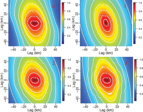
Figure 4. Variation of the anisotropy ratio with the lag distance of the regional options parameter sets using radar data.

As expected, the correlogram parameters estimated using the gauged and radar data show appreciable differences (see Table 2 for the REG_1 option). For all cases, the correlation length (L_u) of the gauged data was shorter than the radar counterpart. Also, for the majority of cases the anisotropy ratio (η) of the gauged data was higher than the radar data. There were significant differences in the anisotropy direction (θ) which may not matter much for η > 0.9. The nugget (1 – a_n) for the gauged data varied between 0.03 and 0.13 but has a maximum value of 0.01 for the radar cases. These observed variations could be used to adjust gauged parameter sets to reflect the radar values. The significance of these observed parameter set variations on the kriging results is discussed in a later section.

Table 2. Estimated correlogram parameters defined in equation (4) of the regional option 1 using gauge and radar data. L_u: major axis correlation length; η: anisotropy ratio; θ: anisotropy direction; a_n: correlogram sill.

Date	Lu (km)		η		θ (degrees)		an
	Gauge	Radar	Gauge	Radar	Gauge	Radar	Gauge	Radar
14 January 2014	22.1	35.6	0.78	0.60	5	122	0.87	1.00
20 February 2014	22.6	66.3	0.88	0.42	80	130	0.90	1.00
24 February 2014	22.4	104.3	0.81	0.42	99	97	0.91	1.00
25 February 2014	21.6	61.4	0.81	0.60	0	96	0.89	1.00
05 March 2014	23.8	84.2	0.91	0.49	93	103	0.90	1.00
09 March 2014	9.7	39.9	0.83	0.82	108	141	0.97	0.99
10 March 2014	18.4	54.2	0.86	0.59	84	97	0.94	1.00
25 March 2014	18.7	30.3	0.91	0.79	90	113	0.90	1.00
26 March 2014	17.6	20.4	0.67	0.89	99	93	0.94	1.00
27 March 2014	19.7	60.2	0.88	0.77	133	70	0.92	1.00
28 March 2014	19.4	40.9	0.65	0.59	106	121	0.95	1.00
14 April 2014	28.1	40.0	0.63	0.84	4	11	0.88	1.00

3.2 LVA options parameter sets

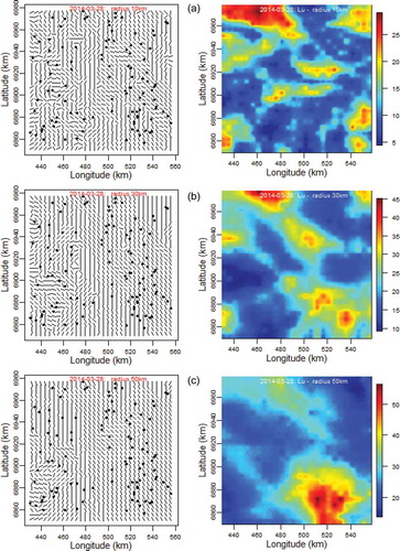
Figure 5 compares the LVA directions and correlation lengths of options LVA_1, LVA_3 and LVA_5. Undoubtedly, the LVA parameter sets do show significant variations over the study area, and, as expected, the variability is smoothed out as the radial distance increases. To our knowledge no such detailed analysis of radar images has been carried out before. However, it is yet to be seen whether the observed LVA parameter set variations have any significant effect on the kriging interpolation. Evaluation of the correlogram options was carried out and is presented in the next section.

Figure 5. Locally varying anisotropy (LVA) direction (θ, left panels) and the major axis correlation length (L_u in km, right panels), for radii of (a) 10 km, (b) 30 km and (c) 50 km.

3.3 Cross-validation results

Results of the cross-validation explained in Section 2.4 were used to calculate the performance statistics. For each station, both the mean and variance were obtained in the Gaussian domain. Normal quantiles (Q_p) of the appropriate probability (p) were used to define the median (Q_0.5), inter-quartile range (Q_0.75–Q_0.25) and 90% prediction limits (Q_0.05, Q_0.95). These values were then converted into rainfall estimates in mm using the empirical distribution approach described in Section 2.1. The performance statistics were:

• root-mean-square-error (RMSE) defined as:

  (9)

• mean-bias (MB) defined as:

  (10)

• mean-absolute-bias (MAB) defined as:

  (11)

• mean-inter-quartile-range (MIQR) defined as:

  (12)

where V_O(i) and V_E(i) are the observed and estimated median values of gauge i, V_E75 and V_E25 are the upper and lower quartiles of the estimates, and N is the number of gauges. The mean standard deviation (SD) in the Gaussian domain was also used as one of the performance statistics.

Figure 6 compares the cross-validation median estimates with the observed for three events for the REG_1 option. A few gauge station values, lying outside the prediction limits, were difficult to predict. While an increase in k improves the estimates, it was observed that it did not matter which k-fold was used as they all gave similar rankings of the correlogram option. Table 3 presents the performance statistics for two events of the 10-fold cross-validation. To get a better picture of the relative performance of correlogram options over all wet days examined, the various statistics values for each day were ranked from the least (best, 1) to the highest (worst, 14) as shown in Table 4 for one of the days. These ranks were then summed for each statistic and correlogram option to obtain a composite sum which was also ranked to obtain a final table of performance ranking (Table 5).

Table 3. Estimated performance statistics using the different correlograms for two wet days, 10-fold case. RMSE: root mean square error; MB: mean bias; MAB: mean absolute bias; MIQR: mean inter quartile range; SD: mean standard deviation in the Gaussian domain.

Correlogram option	24/02/2014					28/03/2014
	RMSE	MB	MAB	MIQR	Mean SD	RMSE	MB	MAB	MIQR	Mean SD
Gauge
G_REG_0	1.74	−0.35	1.05	2.27	0.66	37.03	−4.42	21.5	47.4	0.68
G_REG_1	1.69	−0.28 −0.32	1.06	2.32	0.66	37.31	−4.05	21.4	46.9	0.68
G_REG_2	1.70		1.04	2.31	0.66	37.38	−4.05	21.4	46.9	0.68
G_REG_3	2.04	−0.60	1.29	2.66	0.78	36.46	−3.78	20.8	46.7	0.67
Radar
R_REG_0	1.96	−0.13	1.21	1.05	0.29	38.42	−3.34	21.4	29.6	0.43
R_REG_1	1.94	−0.04	1.21	1.12	0.32	38.19	−3.31	21.8	32.1	0.47
R_REG_2	1.85	−0.08	1.16	1.13	0.32	38.30	−3.23	21.8	32.2	0.47
R_REG_3	1.77	−0.11	1.12	1.11	0.31	38.44	−3.81	21.9	34.2	0.52
LVA
R_LVA_0	1.69	−0.25	1.11	2.39	0.77	37.05	−3.92	20.9	43.9	0.63
R_LVA_1	1.88	−0.49	1.16	2.90	0.88	38.29	−4.26	22.6	53.0	0.76
R_LVA_2	1.76	−0.38	1.11	2.71	0.84	37.07	−3.64	21.5	49.4	0.70
R_LVA_3	1.74	−0.28	1.14	2.44	0.78	37.18	−3.81	21.1	45.1	0.65
R_LVA_4	1.71	−0.19	1.11	2.26	0.74	37.87	−3.78	21.3	41.9	0.61
R_LVA_5	1.80	−0.22	1.17	2.03	0.70	38.09	−4.07	21.6	39.9	0.58

Table 4. Ranked performance statistics for the correlograms, where 1 denotes best and 14 worst: 10-fold case for 24 February 2014. RMSE: root mean square error; MB: mean bias; MAB: mean absolute bias; MIQR: mean inter quartile range; SD: standard deviation in the Gaussian domain; correlogram option prefix G for gauged and R for radar.

Correlogram option	RMSE	MB	MAB	MIQR	Mean SD
G_REG_0	5	4	2	7	5
G_REG_1	2	6	3	9	5
G_REG_2	3	5	1	8	7
G_REG_3	14	1	14	12	11
R_REG_0	13	11	13	1	1
R_REG_1	12	14	12	3	4
R_REG_2	10	13	10	4	3
R_REG_3	8	12	7	2	2
R_LVA_0	1	8	5	10	10
R_LVA_1	11	2	9	14	14
R_LVA_2	7	3	4	13	13
R_LVA_3	5	7	8	11	12
R_LVA_4	4	10	6	6	9
R_LVA_5	9	9	11	5	8

Table 5. Ranked performance statistics for the correlograms (1 for best and 14 for worst): 10-fold case over all 12 wet days. See Table 4 for abbreviations.

Correlogram option	RMSE	MB	MAB	MIQR	Mean SD
G_REG_0	1	8	1	7	6
G_REG_1	3	4	4	9	8
G_REG_2	2	6	3	8	5
G_REG_3	9	2	14	12	11
R_REG_0	13	14	13	1	1
R_REG_1	14	13	11	3	3
R_REG_2	11	12	10	2	2
R_REG_3	10	11	7	4	4
R_LVA_0	5	7	4	10	10
R_LVA_1	12	1	12	14	14
R_LVA_2	8	3	9	13	13
R_LVA_3	6	5	8	11	12
R_LVA_4	7	9	6	6	9
R_LVA_5	4	10	2	5	7

Figure 6. Comparison of the cross-validation median estimates (solid [blue] line) and the observed values (open circles) for correlogram option R_REG_1. The (red) dotted lines represent the 90% prediction limits. Gauge numbers are in increasing order of the median prediction for easy visualisation.

As observed in Table 3, the performance statistics of RMSE, MB and MAB did not discriminate significantly among the various correlogram options as they all performed satisfactorily. The mean standard deviation, representing the uncertainty in the estimations and used to estimate MIQR, has been identified as the most discriminatory statistic. Clearly, the regional options for the radar data outperformed the gauged data, signifying the improvements achieved by deriving the correlogram from radar data. The results for regional options 1 to 3 were very close to those based on the correlogram map (REG_0), suggesting a good fit of the 2D exponential distribution. Disappointingly, the LVA options performed worse than the regional options, but it improved with increasing circle radius within which data were sourced. This demonstrates that incorporation of the LVA observed in the radar data may not help to improve the estimates, the most import thing being the overall picture of the spatial structure.

These results were confirmed by conditional simulation of the random rainfields where simulated grid data were included in the kriging of the target node. 120 rainfields were simulated for each correlogram option, leaving out one of the k – 10 subsamples at a time. Values of the grid nodes of the observed k – 10 subsample eliminated were then extracted from the simulated rainfields. This was repeated for all subsamples, results combined, and analysed as done for the purely kriging case. While there were subtle changes in numerical values, the results were nearly identical with the purely kriging case as demonstrated in Fig. 7 and Table 6 which provides the overall raking of the correlogram options.

Table 6. Ranked performance statistics for the correlograms (1 for best and 14 for worst): 10-fold case over all 12 wet days and by conditional simulation. See Table 4 for abbreviations.

Correlogram Option	RMSE	MB	MAB	MITQR	Mean SD
G_REG_0	1	1	1	10	9
G_REG_1	2	3	3	6	6
G_REG_2	3	8	5	8	5
G_REG_3	5	1	10	9	8
R_REG_0	12	14	8	1	1
R_REG_1	14	13	7	4	4
R_REG_2	10	12	4	2	2
R_REG_3	8	11	2	3	3
R_LVA_0	7	7	11	13	13
R_LVA_1	13	3	14	14	14
R_LVA_2	11	5	13	12	12
R_LVA_3	9	6	12	11	11
R_LVA_4	5	9	9	7	10
R_LVA_5	4	10	6	5	7

Figure 7. Comparison of the cross-validation median estimates (solid [blue] line) and the observed values (open circles) for correlogram option R_REG_1 by conditional simulation. See Fig. 6 for explanation.

4 Concluding remarks

This paper investigates the use of radar information to improve interpolation of scattered gauged daily rainfall data over a gridded catchment. The study area is within the Mt. Stapylton (near Brisbane, Queensland) weather radar range which is a 1500 S-band Doppler type. Gauged and rainfall data for the first four months of 2014 were analysed. Fourteen different ways of developing and fitting correlograms in the Gaussian domain from the radar (or gauged) data were compared using three k-fold cross-validations. These included a regional correlogram where all values within the radar fields (or gauged data) were used, as well as locally varying correlograms developed from radar data within a set radius of the target pixel. All correlogram maps were developed using the “round-trip” Fast Fourier Transform method. Since one of the objectives of the research project is to transfer the results to data poor regions where radar data may not be available, a two-dimensional four-parameter (sill, major axis correlation length, anisotropy ratio and direction) exponential distribution was fitted to the correlograms in different ways, specifically within and between concentric circles and for the whole correlogram maps. The main findings of the paper are:

• Comparing the gauged, collocated radar and full radar data, it was observed that the wetted area ratios and the maximum wet gauge/pixel amounts were different for the datasets of the same day, while there is similarity between the average wet gauge amount of the collocated and the full radar values that could be exploited for screening simulated rainfields.

• There were significant differences between the correlogram parameters estimated using radar and gauged data, even though the gauged network density is considered to be one of the highest in Australia. Specifically, the major axis correlation lengths (L_u) of the radar data were longer than those based on the gauged data, anisotropy was more pronounced in radar data, and no obvious trend was evident in the anisotropy direction differences.

• The most important statistic that discriminated significantly among the various correlogram options was the mean standard deviation which represents the uncertainty in the kriging estimates and was used to calculate the mean inter-quartile statistic.

• The regional options for the radar data outperformed the gauged data, signifying the improvements achieved by incorporating radar information in ordinary kriging.

• The radar images exhibit a considerable locally varying anisotropy. However, incorporation of the locally varying anisotropy in the kriging interpolation and conditional simulation did not improve the estimates as judged by performance statistics.

It needs to be underlined that the methodology for the interpolation process is automated and, at this stage, the intention is for understanding the relationship between radar and gauged rainfall with the hope of interpolating the existing long-term gauged records for meaningful long-term hydrological modelling. Extension to real time forecasting should not pose a problem, particularly where sub-daily timescale is considered. It is intended to analyse more radar images and to establish the variability of runoff on catchments by running simulated conditional rainfields through a rainfall-runoff model. Application of the concepts to finer timescale by daily rainfall disaggregation methods (e.g. Gyasi-Agyei and Mahbub 2007, Gyasi-Agyei 2011) is also being considered.

Acknowledgements

Dr Alan Seed of the Australian Bureau of Meteorology is thanked for providing the radar data.

Disclosure statement

No potential conflict of interest was reported by the author.

References

- Austin, P.M., 1987. Relation between measured radar reflectivity and surface rainfall. Monthly Weather Review, 115 (5), 1053–1070. doi:10.1175/1520-0493(1987)115<1053:RBMRRA>2.0.CO;2
- Bárdossy, A. and Pegram, G.G.S., 2009. Copula based multisite model for daily precipitation simulation. Hydrology and Earth System Sciences, 13, 2299–2314. doi:10.5194/hess-13-2299-2009
- Bitew, M.M. and Gebremichael, M., 2011. Assessment of satellite rainfall products for streamflow simulation in medium watersheds of the Ethiopian highlands. Hydrology and Earth System Sciences, 15, 1147–1155. doi:10.5194/hess-15-1147-2011
- Cressie, N., 1993. Statistics for spatial data. New York: John Wiley and Sons.
- Duan, Q., Sorooshian, S., and Gupta, V., 1992. Effective and efficient global optimization for conceptual rainfall- runoff models. Water Resources Research, 28 (4), 1015–1031. doi:10.1029/91WR02985
- Ehret, U., et al., 2008. Radar-based flood forecasting in small catchments, exemplified by the Goldersbach catchment, Germany. International Journal of River Basin Management, 6 (4), 323–329. doi:10.1080/15715124.2008.9635359
- Gómez-Hernández, J.J. and Journel, A.G., 1993. Joint sequential simulation of multi-Gaussian fields. Geostatistics Troia, 92 (1), 85–94.
- Goovaerts, P., 2000. Geostatistical approaches for incorporating elevation into the spatial interpolation of rainfall. Journal of Hydrology, 228 (1–2), 113–129. doi:10.1016/S0022-1694(00)00144-X
- Gyasi-Agyei, Y., 2011. Copula-based daily rainfall disaggregation model. Water Resources Research, 47 (7), W07535. doi:10.1029/2011WR010519
- Gyasi-Agyei, Y. and Mahbub, P.B., 2007. A stochastic model for daily rainfall disaggregation into fine time scale for a large region. Journal of Hydrology, 347, 358–370. doi:10.1016/j.jhydrol.2007.09.047
- Gyasi-Agyei, Y. and Pegram, G., 2014. Interpolation of daily rainfall networks using simulated radar fields for realistic hydrological modelling of spatial rain field ensembles. Journal of Hydrology, 519, 777–791. doi:10.1016/j.jhydrol.2014.08.006
- Isaaks, E.H. and Srivastava, R.M., 1990. An introduction to applied geostatistics. Oxford: Oxford University Press.
- Jeffrey, S.J., et al., 2001. Using spatial interpolation to construct a comprehensive archive of Australian climate data. Environmental Modelling and Software, 16 (4), 309–330. doi:10.1016/S1364-8152(01)00008-1
- Krajewski, W.F., 1987. Cokriging radar-rainfall and rain gage data. Journal of Geophysical Research: Atmosphere, 92 (D8), 9571–9580. doi:10.1029/JD092iD08p09571
- Krajewski, W.F., Villarini, G., and Smith, J.A., 2010. Radar-rainfall uncertainties. Bulletin of the American Meteorological Society, 91, 87–94. doi:10.1175/2009BAMS2747.1
- Ly, S., Charles, C., and Degré, A., 2011. Geostatistical interpolation of daily rainfall at catchment scale: the use of several variogram models in the Ourthe and Ambleve catchments, Belgium. Hydrology and Earth System Sciences, 15, 2259–2274. doi:10.5194/hess-15-2259-2011
- Quirmbach, M. and Schultz, G.A., 2002. Comparison of raingauge and radar data as input to an urban rainfall–runoff model. Water Science and Technology, 45 (2), 27–33.
- Rabiei, E. and Haberlandt, U., 2015. Applying bias correction for merging raingauge and radar data. Journal of Hydrology, 522, 544–557. doi:10.1016/j.jhydrol.2015.01.020
- Rosenblueth, E., 1975. Point estimates for probability moments. Proceedings of the National Academy of Sciences, 72 (10), 3812–3814. doi:10.1073/pnas.72.10.3812
- Sinclair, S. and Pegram, G.G.S., 2005. Combining radar and raingauge rainfall estimates using conditional merging. Atmospheric Science Letters, 6 (1), 19–22. doi:10.1002/(ISSN)1530-261X
- Teegavarapu, R.S.V. and Chandramouli, V., 2005. Improved weighting methods deterministic and stochastic data-driven models for estimation of missing precipitation records. Journal of Hydrology, 312, 191–206. doi:10.1016/j.jhydrol.2005.02.015
- Velasco-Forero, C.A., et al., 2009. A non-parametric automatic blending methodology to estimate rainfall fields from raingauge and radar data. Advances in Water Resources, 32, 986–1002. doi:10.1016/j.advwatres.2008.10.004
- Verworn, A. and Haberlandt, U., 2011. Spatial interpolation of hourly rainfall - effect of additional information, variogram inference and storm properties. Hydrology and Earth System Sciences, 15, 569–584. doi:10.5194/hess-15-569-2011
- Wang, L.-P., et al., 2013. Radar-raingauge data combination techniques: a revision and analysis of their suitability for urban hydrology. Water Science and Technology, 68 (4), 737–747. doi:10.2166/wst.2013.300
- Yao, T. and Journel, A.G., 1998. Automatic modeling of (cross) covariance tables using fast Fourier transform. Mathematical Geology, 30 (6), 589–615. doi:10.1023/A:1022335100486