Understanding flow dynamics and density currents in a river-reservoir system under upstream reservoir releases

ABSTRACT

A three-dimensional flow and temperature model was applied for a 124 km river-reservoir system from Lewis Smith Dam tailrace to Bankhead Lock & Dam, Alabama. The model was calibrated against measured water levels, temperatures, velocities and flow rates from 4 May to 3 September 2011 under small constant release (2.83 m³/s) and large intermittent releases (~140 m³/s) from an upstream reservoir. Distributions of simulated flow and temperatures and particle tracking at various locations were analyzed which revealed the complex interactions of density currents, dynamic surface waves and solar heating. Flows in the surface and bottom layers moved in both upstream and downstream directions. If there was small constant release only from Smith Dam, simulated bottom temperatures at Cordova were on average 4.8°C higher than temperatures under actual releases. The momentum generated from large releases pushed bottom density currents downstream, but the released water took several days to reach Cordova.

Editor D. Koutsoyiannis; Associate editor B. Dewals

KEYWORDS:

• density currents
• reservoir releases
• simulations
• flow characteristics
• temperature
• solar heating
• particle tracking

1 Introduction

River regulation as a means of water resources management is a common operating procedure all over the world. Reservoir release is becoming a prominent characteristic for regulated rivers to meet hydro-electric power demands (Petts et al. 1985). Increasing flow release leads to larger flow depths at downstream river, where rapid stage changes of more than 1 m are common. Stage changes have been detected more than 100 km downstream of the large dams after the wave attenuation (Petts 1984). Operational constraints considering water temperature in downstream river focused on a minimum flow requirement for water quality and temperature control (Carron and Rajaram 2001). The need for minimum flow is usually during the warm season of the year, especially during the summer, to maintain lower water temperatures downstream (Wunderlich and Shiao 1984, Consultants 1986). Atmospheric conditions have a large effect on river temperature after the reservoir release. Due to solar heating, water temperature in a shallow river is typically much warmer than the release temperature of stored water in the reservoir.

Toffolon et al. (2010) used a coupled hydro-thermodynamic deterministic model, and analytical solutions for river water temperature have been developed to get a better insight into the physical properties associated with the propagation of both hydrodynamic and thermal peaking waves in the downstream receiving river. The hydro-wave and thermal wave dynamics are rather complex, propagation of the thermal wave is always slower than the hydrodynamic wave, and the two waves are slowly damped. The study by Toffolon et al. (2010) does not consider the formation of density currents in the receiving river.

A significant number of river-reservoir systems all over the world have large diurnal variations in atmospheric heating rates and develop density currents in the downstream river/reservoir due to colder denser flow releases from an upstream reservoir. A plunging density current occurs when the density of the water flowing into a reservoir or lake is greater than the density of the ambient water. In the riverine portion of a reservoir, the denser inflow mixes homogeneously with the reservoir or lake water first due to the inflow momentum. When the inflow momentum diminishes, the inflowing water eventually plunges under the ambient water and flows along the bottom as a density current (Farrell and Stefan 1989). The intermittent denser flow releases from an upstream reservoir create very complex and unsteady density currents that are not well understood yet.

Many laboratory and numerical model studies focusing on density currents have been conducted in the last decades. Density currents have been studied in situ by various researchers (Serruya 1974, Smith 1975, Carmack et al. 1979, Fischer and Smith 1983, Alavian and Ostrowski 1992, Chikita 1992, Dallimore et al. 2001). The density currents were also investigated in the laboratory (Akiyama and Stefan 1984, Hauenstein and Dracos 1984, Alavian 1986, Hallworth et al. 1996). Most studies in the past dealt with sloping channels having a rectangular cross-section, and various simplifying assumptions were made to develop analytical models with laboratory data to understand density currents (Singh and Shah 1971, Savage and Brimberg 1975, Denton 1985, Kranenburg 1993, Fernandez and Imberger 2008a, 2008b).

A one-dimensional integral model was developed by Fang and Stefan (2000) for a discharge from a channel over a horizontal or a sloping bottom into a reservoir or a lake to determine dilution up to plunging for density current computations. Two-dimensional hydrodynamic models were developed to study density current by assuming that the density current does not participate in the dynamics of heating and mixing but the entrainment takes place from the ambient reservoir into the downflow (Imberger and Patterson 1980, Buchak and Edinger 1984, Jokela and Patterson 1985). Gu (2009) used a validated two-dimensional (2D) simulation model CE-QUAL-W2 (Cole and Wells 2010) to quantify systematically the effects of inflow and ambient parameters on the behavior of a density-induced contaminant current in various flow regimes in a stratified reservoir through numerical experiments. Several studies about three-dimensional (3D) gravity currents were conducted recently using laboratory data and numerical models (Imran et al. 2007, Firoozabadi et al. 2009, Rueda and MacIntyre 2010, An and Julien 2014). Rueda and MacIntyre (2010) used a 3D free surface hydrodynamic model with fine grid resolution to simulate negatively buoyant density currents on steep bottoms with varying slopes in Toolik Lake, AK.

In the last several decades, 3D Environmental Fluid Dynamics Code (EFDC) (Hamrick 1992) has been widely used in modeling river, estuarine and coastal hydrodynamics and transport processes. In order to quantify numerical and modeled entrainment, Kulis and Hodges (2006) explored the grid resolution required in EFDC to capture gravity current motions in an idealized basin with and without a turbulence closure. The study basin was scaled and based on a shallow bay, Corpus Christi Bay in Texas, USA, which is affected by the underflow from Oso Bay. Liu and Garcia (2008) used a modified 3D EFDC model to simulate the density current and bi-directional flows in the Chicago River system.

None of the studies considered dynamic releases from an upstream reservoir and heat exchange from the atmosphere in a river-reservoir system at the same time. A simple numerical or laboratory study cannot reveal the complex processes and interactions such as cooling, heating and flow dynamics (mixing and density current movement). In this paper, the 3D EFDC model was applied and calibrated in a river-reservoir system from the Smith Dam tailrace (SDT, Fig. 1) to the Bankhead Lock & Dam (BLD) in Alabama (AL), USA. The calibrated model was then used to investigate the unsteady flow dynamics focusing on density current movement and heat transport under varying reservoir releases and atmospheric heat exchange due to diurnally varying solar radiation and air temperature.

Figure 1. (a). Geographic location of the study area and the location of Birmingham weather station used for the study, (b) Longitudinal bottom elevation along the centerline of BRRS and water surface elevation after a large release from the Smith Dam tailrace to Bankhead Lock & Dam, (c) Color contours of the bottom elevation showing Sipsey Fork, the lower Mulberry Fork, and Black Warrior River as the model simulation domain; two monitoring stations (Cordova and GOUS), model upstream and downstream boundary locations: Smith Dam tailrace (SDT) and Bankhead L&D (BLD), three locations for reporting simulation results (MSF, UPJ and MJC, Table 2).

2 Materials and methods

2.1 Study area

The study deals with flow and temperature simulations in a river-reservoir system (124.2 km) from SDT (upstream flow boundary) to BLD (downstream water level boundary) in Walker County, AL, USA (Fig. 1). The river reach includes Sipsey Fork (21.9 km), the lower Mulberry Fork (70.6 km), and a reservoir segment (31.7 km) of Bankhead Lake (Fig. 1), which is also called Black Warrior River. Sipsey Fork and the lower Mulberry Fork are the riverine portions of Bankhead Lake, therefore, the study area is referred here as the Bankhead river-reservoir system (BRRS). The Black Warrior River is formed about 40 km west of Birmingham by the confluence of the Mulberry Fork and the Locust Fork, which join as arms of Bankhead Lake, a narrow reservoir formed by BLD. The Black Warrior River is impounded by a series of locks and dams to form a chain of reservoirs that not only provide a path for an inland waterway, but also yield hydroelectric power, drinking water and industrial water.

The EFDC model was applied to simulate unsteady flow patterns and temperature distributions in BRRS including the intake canal and the discharge canal of a power plant (Fig. 1(c)) near Parrish, AL. The water surface elevation in BRRS depends on water releases from Smith Dam, flows from its tributaries (e.g. Locust Fork, Lost Creek and Blackwater Creek) and the water surface elevation in BLD influenced by outflow through hydro turbines, spillage through gates of BLD and loss of water through the Bankhead navigation lock. The bottom elevations of the centerline of BRRS ranged from about 59.5 to 77.2 m a.m.s.l. (using NAVD 1988 datum, Fig. 1(b)). The average bottom slope is 0.00014 but there are local slope variations (ranging from −0.002 to 0.002 over each ~2 km distance) as shown in Fig. 1(b) (having different scales in depth and distance). Bottom slopes in BRRS are much smaller than steep bottom slopes (0.03–0.2) in Toolik Lake (Rueda and MacIntyre 2010). A typical water surface profile after a large release from Smith Dam displayed in Fig. 1(b) depicts the response of water level increase in the upstream portion of BRRS only.

The water releases from Smith Dam to BRRS are normally 2.83 m³/s, but during later spring, summer and early fall, intermittent water releases of high discharges (Table 1) are practiced to meet peak electric generating demand. During the normal water releases, water depths in Sipsey Fork range from 2.16 to 4.55 m, in the lower Mulberry Fork from 4.71 to 11.47 m, and in the Black Warrior River (Bankhead Lake) from 12.12 to 17.73 m. The water surface elevation at BLD is about 77.66 m a.m.s.l. (Fig. 1(b)).

The monitoring stations and cross-sections for result analysis are shown in Fig. 1(c) and summarized in Table 2. The middle cross-section of Sipsey Fork (MSF) is located at 11.1 km downstream from SDT. The cross-section at a short distance (0.64 km) upstream of the junction of Sipsey Fork and the upper Mulberry Fork is called UPJ. The middle section between the junction and Cordova is called MJC. The monitoring station at 5.58 km upstream of the power plant is called GOUS (Fig. 1(c)).

Table 1. Statistical summary of the intermittent flow releases from Smith Dam.

Statistical parameters	Starting time of release (hour)	Duration of release (hour)	Average release flow rate (m^3/s)
Minimum	4.83	0.17	104.02
25^thpercentile	12.02	3.63	137.30
Median	13.02	4.42	138.76
75^thpercentile	14.02	6.17	142.05
Maximum	20.25	116.17	273.54
Average	12.97	6.86	148.69
Standard deviation	2.42	14.38	33.92

Table 2. Description and abbreviation of cross-sectional locations used in the study (Fig. 1(c)).

Abbreviation	Description
Cordova	USGS monitoring station at Cordova on the lower Mulberry River
GOUS	Monitoring station upstream from the power plant
MSF	Middle cross-section of Sipsey Fork
UPJ	Just upstream of the junction of Sipsey Fork and the upper Mulberry Fork
MJC	Middle cross-section between the junction and Cordova
SDT	Smith Dam tailrace (upstream boundary of EFDC model)
BLD	Bankhead Lock & Dam (downstream boundary of EFDC model)

2.2 Hydrodynamic model

The study deals with a relatively narrow river-reservoir system, which could be modeled using a 2D longitudinal-vertical hydrodynamic and water quality model, such as CE-QUAL-W2 model (Cole and Wells 2010). To more accurately simulate complex flow and temperature distributions in BRRS, especially near the power plant, the 3D EFDC hydrodynamic model was applied for the project to understand the hydrodynamics of density currents formed by upstream reservoir releases. The EFDC model is a general purpose modeling package that can be configured to simulate 1D, 2D, and 3D flow, transport and biogeochemical processes in various surface water systems including rivers, lakes, estuaries, reservoirs, wetlands and coastal regions (Shen and Lin 2006, Çalışkan and Elçi 2009, Jeong et al. 2010, Wang et al. 2010, Kim and Park 2012, Devkota and Fang 2015). The EFDC model was originally developed at the Virginia Institute of Marine Science and the version of EFDC used for the study with pre- and post-processing tools was EFDC-DSI (Craig 2010) from the Dynamic Solutions-International, LLC (http://efdc-explorer.com/). EFDC solves three-dimensional turbulent-averaged equations of motions for a variable-density fluid. EFDC’s hydrodynamics are based on the 3D hydrostatic equations formulated in curvilinear-orthogonal horizontal coordinates and a sigma vertical coordinate system. The Mellor-Yamada level 2.5 turbulence closure scheme (Mellor and Yamada 1982) is used to calculate turbulence parameters; vertical turbulent diffusion coefficients of momentum and mass. The horizontal eddy viscosity, A_H is calculated using the Smagorinsky subgrid scale scheme (Smagorinsky 1963), which can be written in the two-dimensional Cartesian coordinate as:

(1)

where is horizontal mixing constant, and are model grid sizes in x and y directions, u and v are velocity components in x and y directions. The numerical scheme used in EFDC to solve the momentum equations uses a second-order accurate spatial finite difference on a staggered or C grid. The time integration is implemented using a second-order accurate three-time level, semi-implicit finite difference scheme with an internal-external mode splitting scheme to separate the internal shear or baroclinic mode from external free surface gravity wave or barotropic mode. Details of governing equations and numerical schemes for EFDC hydrodynamic model are given by Hamrick (1992).

2.3 Model setup

The EFDC horizontal model grids developed for BRRS were based on the NAVD 1988 horizontal datum and Universal Transverse Mercator (UTM) projection coordinate system. The horizontal grids were developed using the shoreline GIS shapefile of the Black Warrior River downloaded from AlabamaView (http://www.alabamaview.org/). The shoreline data were further validated using AutoCAD data and hydrographic data developed by the US Army Corps of Engineers (USCOE).

The EFDC model applied for the study area has a total of 6974 curvilinear orthogonal grids and 10 horizontal layers (determined through a sensitivity analysis) along the depth direction; therefore, there are a total of 69 740 computational cells. The bathymetry was based on hydrographic data in an AutoCAD file for intake and discharge canals of the power plant; x, y and z coordinates from USCOE for Black Warrior River and the lower Mulberry Fork; and HEC-RAS geometry file for Sipsey Fork. The grid size ∆X in transverse direction along the river ranged from 9.5 m to 189.8 m and ∆Y in longitudinal flow direction ranged from 10.0 m to 277.1 m. Average grid sizes ∆X and ∆Y were 25.7 m and 100.9 m, respectively. The horizontal layer thicknesses (∆Z) ranged from ~0.2 m to ~1.8 m. Sipsey Fork near the upstream boundary was represented by two to three grid cells along the cross-section. The reservoir cross-sections near BLD are much wider than cross-sections at other river reaches of BRRS. Therefore, there are eight grid cells along the cross-section near BLD to better represent the bathymetric details. The simulation domain includes grid cells to represent four tributaries flowing into BRRS (Blackwater Creek, the upper Mulberry Fork, Locust Fork, and Lost Creek) where streamflow measurements were available from the US Geological Survey (USGS) gauging stations. The model also designates specific cells for direct flow inputs from 15 relatively small streams where simulated hydrographs from a watershed model were available (Weems 2013). The model includes withdrawal and return flow boundaries (Hamrick and Mills 2000) to simulate withdrawals and discharges for power plant operations.

2.4 Unsteady boundary conditions

The EFDC model applied for BRRS was run from Julian Day (JD) 104 to 304 in 2011 (i.e. 14 April to 31 October) because of available input data. The majority of observed data available for the project at various monitoring stations (Table 2) were from JD 124 to 246 in 2011 (i.e. 4 May to 3 September, Fig. 2). The upstream boundary of the EFDC model used one-minute time-series data (unsteady) of water releases (m³/s) at SDT (Fig. 2(a)). There are two types of water releases from Smith Dam: (1) more or less constant continuous release (2.83 m³/s) to support the downstream environment and ecosystem; (2) intermittent releases from hydro-turbine units of Smith Dam in order to meet peak electric generation demand (Fig. 1). During the simulation period, total volume of constant water release was 49.4 × 10⁶ m³ and intermittent releases were 588.6 × 10⁶ m³. Therefore, constant water release with lower temperature (8–9°C) was about 7.7% of the total release from Smith Dam. The intermittent releases from Smith Dam had average discharge of about 140 m³/s that lasted about 4 h and started around 13:00 h (Table 1). The study was performed to reveal how these intermittent releases create and affect density currents near the river bottom.

Figure 2. Time-series plots of (a) upstream unsteady flow releases at SDT, (b) upstream temperature boundary conditions at SDT and (c) downstream water surface elevation (m) at BLD in 2011.

Figure 2(b) shows a time-series plot of measured water temperatures at SDT used as the upstream temperature boundary. Water temperatures at the tailrace from 4 May to 3 September increased from 8 to 9°C during the constant release, and water temperatures during the intermittent large releases were 12–14°C, which were 4–5°C higher than temperatures during the constant release only from Smith Dam. This is because constant release occurred from a deep water depth and intermittent releases were from a shallower depth of Smith Dam; and there was lower water temperature in the hypolimnion due to thermal stratification in the summer.

The downstream boundary of the EFDC model was 15-min water surface elevation (WSE) measured at BLD (Fig. 2(c)). Observed WSEs ranged from 77.35 to 77.75 m from 4 May to 3 September 2011 with an average elevation of 77.59 m (standard deviation of 0.07 m).

The atmospheric boundary condition was meteorological data from the Birmingham regional airport obtained from NOAA’s Southeast Regional Climate Center (SERCC). The data include hourly air temperature, atmospheric pressure, wind speed, wind direction, rainfall and cloud cover. Required solar radiation data were not available from SERCC but obtained from Cleveland, AL (the closest Auburn Mesonet station from the study area).

3 Model calibration results

The EFDC model applied for BRRS was calibrated from 4 May (JD 124) to 3 September 2011 (JD 246). The model was calibrated for water surface elevation (Fig. 3 and Table 3), water temperature (Fig. 4 and Table 4), velocity and discharge (Fig. 5) at two monitoring stations: Cordova and GOUS (Fig. 1). Two commonly used calibration parameters for flow, bottom roughness height and the dimensionless horizontal momentum coefficient in EFDC were calibrated to obtain the best match between observed and modeled water surface elevations. In this study, the bottom roughness height of 0.02 m was determined during the calibration. The dimensionless horizontal momentum coefficient (C in equation (1)) was calibrated to be 0.0025 for the BRRS EFDC model.

Figure 3. Time-series plot of observed and modeled water surface elevations (m) at the monitoring station Cordova from 4 May to 3 September 2011.

Figure 4. Time-series plots of observed and modeled (a) surface water temperature (°C) at the Cordova monitoring station and (b) bottom temperature at GOUS (Fig. 1 and Table 2).

Figure 5. Time-series plots of observed and modeled average velocity and total discharge at the cross-section of Cordova.

Table 3. Statistics for model performance evaluation on water surface elevation (m) and water temperature (°C) simulations at the Cordova and GOUS monitoring stations.

Location	Observed Mean	Modeled Mean	ME	MAE	RMSE	RE (%)	RRE (%)
Water surface elevation (m)
Cordova	77.633	77.605	−0.028	0.042	0.052	0.05	8.53
GOUS	77.670	77.587	−0.083	0.083	0.088	0.11	20.57
Water temperature (°C)
Cordova (Shallow)	20.19	20.29	0.10	1.41	1.87	6.97	13.33
GOUS (Deep)	19.94	19.38	−0.56	0.87	1.11	4.36	10.49

ME is the mean error between observed and modeled, MAE is the mean absolute error, RMSE is the root mean square error, RE is the relative error that is MAE divided by the observed mean, RRE is the relative RMSE error that is RMSE divided by the observed range (maximum – minimum).

Table 4. Calculated averages and ranges of flow rates and total volumes of water in the bottom layer at MSF, Cordova and GOUS from 1–5 June, 2011.

Locations	Average and range of flow rate (m^3/s)^1	Water flowing downstream (m^3)	Water flowing upstream (m^3)
MSF	2.95 (0.01–10.25)	938 × 10^3	1.9 × 10^3
Cordova	2.50 (0.01–8.64)	624 × 10^3	49.3 × 10^3
GOUS	1.95 (0.04–6.87)	485 × 10^3	56.7 × 10^3

¹Only positive flow rates, which mean the flow moving downstream (BLD), were used to compute averages and ranges of flow rates.

Figure 3 shows the time series plot of measured and simulated WSE at the USGS Cordova monitoring station from 4 May to 3 September 2011. The agreement between observed and modeled WSEs at Cordova is very good with median difference of 0.032 m (Table 3). The average difference (Observed – Modeled) between observed and modeled WSEs at GOUS is −0.076 m (ME in Table 3, negative sign indicates that modeled is larger than observed).

Observed temperatures at the USGS Cordova and GOUS monitoring stations were available from 10 May to 2 September for temperature calibration. Modeled surface temperatures at Cordova follow the trend of observed temperatures over time (Fig. 4(a)) reasonably well. Statistical summary of differences and absolute differences between observed and modeled temperatures at the two stations is given in Table 3. Figure 4(b) shows that modeled bottom temperatures at GOUS closely follow the pattern of the variation of observed bottom temperatures. There are several periods of measured bottom temperature drops at GOUS: a drop from 22.0 to 19.8°C between JD 148 and 150 (28–30 May 2011), a drop from 25.1 to 17.3°C between JD 156 and 161 (5–10 June 2011), a drop from 22.8 to 19.7°C between JD 183 and 189 (2–8 July, 2011), etc. The EFDC model predicted the magnitude and duration of those temperature drops with reasonable accuracy. Average and absolute differences between observed and modeled bottom temperatures at GOUS are 0.56 and 0.87°C (Table 3), respectively. It is essential that the EFDC model can accurately predict the bottom temperatures at GOUS because they are directly related to how the model can accurately predict the density currents along the river bottom, which is the focus of the study and presented in the next section.

In June 2011, flow velocities at Cordova were measured from 22 June, 10:50 h, to 23 June, 09:25 h (approximately one day) using Acoustic Doppler Current Profiler (ADCP). The ADCP data were processed using a velocity mapping software VMS (Kim et al. 2009) to obtain cross-sectional average velocities and discharge (Fig. 5), which were compared with modeled results at Cordova from the EFDC model. Negative velocity in Fig. 5(a) indicates the flow direction from downstream towards upstream. Visually, modeled mean velocities matched reasonably well with observed mean velocities (Fig. 5(a)). Modeled and measured discharges match reasonably well and exhibit the response of the large release from Smith Dam from 22 June, 17:00 to 19:00 h (lasted 2 hrs with a flow rate of 143.13 m³/s). It can be inferred that the discharge at Cordova started to increase roughly 2.5–3.0 hrs after the large release at Smith Dam. Observed peak discharge at Cordova was about 70 m³/s (attenuated from 143 m³/s) and the discharge wave (increasing and decreasing) moving towards downstream lasted about 9 hrs at Cordova in response to the two-hour release at Smith Dam.

4 Simulation results of flow properties and density currents

4.1 Velocity and flow variations

An in-depth analysis of observed data and EFDC modeled results at various locations of BRRS were conducted to understand flow properties and dynamics (formation and propagation) of density currents under different flow releases from Smith Dam. Figure 6 shows time-series of (a) modeled cross-sectional average velocity and water depth, (b) modeled flow rates in the surface (the 10th layer in EFDC model) and bottom (the first layer) layers at MSF (Table 2) from 31 May to 4 June 2011, including the flow releases from Smith Dam. Simulated depth averaged velocity at MSF reached 0.48 m/s during each large release but had very small magnitudes (~ <0.05 m/s) during the constant small release (2.83 m³/s). Simulated water depth at MSF was about 4.7 m during small release and increased to 6.3–6.6 m after large releases (Fig. 6(a)). For each release, average velocity at MSF followed closely with the release pattern and reached more or less constant velocity shortly after the release started, but the water depth continuously increased and reached the maximum level shortly after the end of the release (Fig. 6(a)). Therefore, the flow rates at the surface and bottom layers also continuously increased and reached the maximum values shortly after the end of the release (Fig. 6(b)). The positive discharges meant the flow direction was from upstream (SDT) to downstream (BLD).

Figure 6. Time-series of (a) modeled cross-sectional average velocity and water depth, (b) modeled flow rates in the surface, and bottom layers at the middle of Sipsey Fork from May 31 to 4 June 2011 including the release from Smith Dam.

When there was a daily large flow release from Smith Dam at or after noon, MSF responded with the increase of flow rate relatively quickly. For example, the release on 2 June started at 12:10 h, the flow rate increase started at 13:00 h (50 min later) and the maximum flow rates in the surface and bottom layers occurred at 18:25 h when the release stopped at 18:00 h (Fig. 6). Water depth, velocity, and flow rates gradually and steadily decreased with time after the release stopped, and the recession lasted more than 12 hrs (e.g. lasted up to 06:00 h on 3 June for the release on 2 June). The flows in different layers at MSF were from upstream towards downstream most of the time, but there were short periods (1–3 hrs) with negative surface flows (Fig. 6(b)), i.e. from downstream towards upstream but bottom water still flows from upstream towards downstream.

Figure 7 shows time-series of simulated water surface elevations (WSEs) and cross-sectional average velocities (m/s) at the MSF, UPJ, MJC, Cordova and GOUS (Fig. 1(c) and Table 2) after daily large releases from 3–9 June 2011. The distance from UPJ and MJC is 11.1 km. The water surface levels at MSF and UPJ had direct responses (rise ~2 m at MSF and then fall) from each release of ~140 m³/s, but water surface levels at MJC, Cordova and GOUS showed more complex interactions (fluctuations) between upstream releases and backwater effects from BLD. The releases on 6–7 June were much larger (~ 280 m³/s) and resulted in ~0.5 m rise of WSE at MJC also. Both time series of WSEs and average velocity show that the response of each release lasted 4–6 hrs was about 20–24 hrs at MSF, UPJ and MJC. Due to the backwater effect from BLD, average velocities at Cordova and GOUS had two rises and falls with certain fluctuations afterwards for those daily releases of ~140 m³/s. On 7 and 8 June, average velocities at Cordova and GOUS also increased and then decreased with time when the flow releases was up to 287 m³/s. Simulated flow rate at each individual layer (shown in Fig. 8) provides more information on flow dynamics at different locations.

Figure 7. Time-series of modeled cross-sectional average velocities (m/s) at MSF, UPJ, MJC, Cordova and GOUS (Table 2) after daily large releases from June 3–9.

Figure 8. Time-series of modeled flow rates (major y axis, −20–20 m³/s) in the surface and bottom layers at the Cordova and GOUS monitoring stations including the release from Smith Dam (the secondary y axis with a different scale, 0–200 m³/s) .

Modeled flow rates in the bottom layer and surface layer at Cordova and GOUS monitoring stations (Fig. 8) exhibited many more variations than flow rates at MSF (Fig. 6), which were closely related to the release from Smith Dam. When there was a daily large flow release from Smith Dam, Cordova and GOUS responded with surface-layer flow rate changing from moving upstream (SDT) to moving downstream (BLD) roughly 2–3 hrs after the release. There were no flow releases on 30 and 31 May (Fig. 8), the flow rates in the bottom layer at Cordova and GOUS were very small and moved either upstream or downstream (Fig. 8). After each flow release (especially on 2–4 June), the positive flow rates in the bottom layer indicate the obvious increases of flow moving downstream. The cumulative effects of daily releases were clearly shown at Cordova: the bottom water flux after 13:00 h on 4 June (after two daily releases) moved downstream all the time, and before that time the bottom water moved either upstream or downstream. These daily releases promoted and enhanced the movement of density currents moving from upstream towards downstream. The maximum flow rate moving downstream occurred a few hours after the release stopped. This does not mean that released water from Smith Dam had reached Cordova and GOUS in a few hours after the release, but these flow rate increases occurred due to the momentum transfer or effect due the large releases from Smith Dam.

For the surface flows at Cordova and GOUS, the maximum flow rates moving upstream were almost the same magnitudes as the maximum flow rates moving downstream (14–16 m³/s). The surface flow moving upstream was due to the backwater effect from the downstream boundary–BLD after the flood wave resulting from the large release reached the downstream boundary. Figure 8 shows that the surface water moved in the same or opposite directions as the bottom water at Cordova and GOUS. For example, from 02:45 to 16:30 h on 4 June (the period near two arrows in Fig. 8 (a)) surface water dominantly moved upstream but bottom water (density current) moved downstream at Cordova, which formed a two-layer flow. The total duration of all releases from 1 June to 5 June (4 days) was 22.7 hrs (23.6% of the time) and resulted in 92%, 75% and 75% of the time with the bottom flow (denser and cooler water) moving from upstream towards downstream at MSF (Fig. 6), Cordova and GOUS, respectively.

Average and ranges of flow rates moving towards downstream at the bottom layer at MSF, Cordova and GOUS are summarized in Table 4. When the flow rate was multiplied by the time interval for the data shown in Fig. 8, volume of bottom water moving downstream and upstream were calculated at MSF, Cordova and GOUS from 1 to 5 June and reported in Table 4. Calculated results in the bottom layers indicate that density currents in MSF moved faster than the currents at Cordova and GOUS. Even though there were small amounts of bottom flow moving towards upstream, the density currents at the river bottom did dominantly move towards downstream when there are daily large flow releases.

Figure 9 shows vertical velocity profiles at the centerlines of MSF, UPJ, MJC, Cordova and GOUS at 13:15 h on 7 June (1 hr after the large release began), 22:15 h on 7 June (4 hrs after the large release stopped) and 11:45 h on 8 June (18 hrs after the large release stopped) in 2011. The release on 7 June lasted 6 hrs and had the maximum flow of 287 m³/s at SDT (Fig. 7). When the large flow was released for 1 hr from Smith Dam, the flow momentum began to affect the velocities at MSF where all water moved downstream (positive velocity) with the maximum velocity 0.22 m/s at the surface. The velocities at UPJ, MJC and Cordova indicate that the flow momentum effect did not reach there yet and velocities were small and moved towards downstream or upstream (negative velocity). At the GOUS, the velocities were negative at the surface layer (–0.15 m/s) which means surface flow moved towards upstream due to the backwater effect from the downstream because of the large release on 6 June. The bottom velocities were positive because the density current or flow momentum effect might reach GOUS from the previous day release. When the large flow release stopped for 4 hrs, the flow momentum came close to GOUS when the surface and bottom velocities at GOUS began to increase. The velocities at all five different locations were all positive showing that the entire flow was moving downstream. The velocities increased to 0.4 m/s for the surface layer at MJC. When the large flow release stopped for 18 hrs, the velocities at MSF decreased to less than 0.06 m/s, but the velocities were all positive at MSF: this may be due to the small constant flow release from the Smith Dam or no backwater effect yet. There were more complex flow dynamics at UPJ, MJC, Cordova and GOUS. The small constant flow could not produce strong flow momentum effect on downstream locations but formed a density current along the channel bottom due to lower release temperature, which is indicated by positive velocities at the bottom layers at UPJ. Small negative surface velocities at UPJ might indicate backwater effect reached there.

Figure 9. Vertical velocity profiles at the centerlines (10 layers/cells along depth) of MSF, UPJ, MJC, Cordova and GOUS at 13:15 h on June 7 (1 hr after the large release began), 22:15 h on June 7 (4 hrs after the large release stopped) and 11:45 h on June 8 (18 hrs after the large release stopped) in 2011. Zero velocity is indicated by a vertical line. Positive and negative velocities mean the flow moving downstream (from SDT to BLD) and upstream (from BLD to SDT), respectively.

4.2 Temperature distributions at BRRS

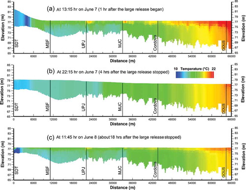
The flow releases from Smith Dam resulted in not only complex flow variations in BRRS but also complex and interesting temperature dynamics and distributions. Figure 10 shows temperature distributions along the channel centerline at BRRS from SDT to GOUS at three different times after a large release on 7 June 2011: (a) 1 h after the large release started (13:15 h), (b) 4 hrs after the large release stopped (22:15 h) and (c) about 18 hrs after the large release stopped. The duration of the large release on 7 June was 6 hrs (Fig. 7, from 12:15 to 18:15 h). The water surface elevation increased from <78 m (a normal condition similar to that in Fig. 10(c) just before the next large release) to about 82 m at SDT at 13:15 h (Fig. 10(a)). The flow momentum pushed colder water downstream about 9 km that is close to the MSF. There are temperature stratifications downstream the MSF due to solar heating and backwater effect (flow) from BLD (Fig. 10(a)). At 4 hrs after the release stopped, the effect of flow momentum seemed to reach GOUS which is about 64 km downstream from SDT (Fig. 10(b)). The water surface elevation dropped to 79.25 m at SDT. It shows there was almost no thermal stratification from SDT to GOUS due to the mixing effect of the flow momentum during the large release and no solar heating during the night. There were temperature gradients from SDT (~12°C) to GOUS (~20°C) as large flow momentum with colder water pushed warmer water in BRRS downstream. Figure 10(c) at 11:45 h on 8 June shows the temperature stratifications were developed almost everywhere after the large release stopped for 18 hrs, which gives temperature distribution just less than 1 hr before the next large release on 8 June. The water surface elevations were almost the same (77.63 m) from SDT to GOUS when there was no large release effect. The small constant inflow (2.83 m³/s) after the large release still pushed the cold water downstream, but the density current near SDT moved very slowly and did not have much effect on water movement further downstream. The cold-water current (blue color) near SDT just moved about 3 km over 18 hrs of small flow release.

Figure 10. Simulated temperature distributions (contours) along the channel centerline of BRRS from SDT to GOUS at three different times after a large release on 7 June 2011: (a) 1 hour after the large release started, (b) 4 hours after the large release stopped and (c) about 18 hours after the large release stopped.

4.3 Temperature variations at Sipsey Fork

Figure 11 shows time-series of air temperature at Birmingham airport and modeled surface and bottom temperatures (15-min model output) at MSF from 31 May to 4 June 2011, including flow releases (m³/s) and temperatures (°C) measured at SDT. When there were no large releases from Smith Dam on 30 and 31 May (Fig. 8), temperature stratification of 5.5°C between surface and bottom layers was developed on 1 June (Fig. 11). There was a short release that lasted for 23 min starting from 12:00 h on 1 June, but the release did not have significant impact on the thermal stratification at MSF (Fig. 11). The second release of 141.7 m³/s on 1 June started from 14:00 h and lasted for 4 hrs and 20 min (4.33 hrs). The flow momentum created by the second release significantly reduced the thermal stratification at MSF (temperature became more or less well mixed). The period of completely mixed condition (assuming surface and bottom temperature difference <0.5°C) started from 15:45 h on 1 June to 07:00 h on 2 June (15 hrs and 15 min). The well-mixed condition at SDT was developed immediately after the large release from Smith Dam, but the well-mixed condition at MSF was developed 1.75 hrs after the release started. It would take about 6 hrs to travel 10.9 km with 0.48 m/s velocity (Fig. 6) from SDT to MSF but actually the velocity decreased from 1.41 m/s at SDT to 0.48 m/s at MSF; therefore, it only took less than 2 hrs to develop the well-mixed condition at MSF. Water temperatures at MSF decreased from 20.9°C at 15:45 h to 12.9°C at 18:20 h (end of the release) because the release had a water temperature of 12°C, and then remained at more or less constant temperature up to 07:00 h on 2 June because of lack of solar heating during the night. Surface temperature at MSF started to increase after 07:00 h due to solar heating and convection/conduction with warm air temperature and reached a maximum temperature of 17.7°C at 12:50 h on 2 June when air temperature increased from 23.9 to 36.7°C. Water temperature in the bottom layer at MSF stayed more or less constant with a small decrease. The temperature stratification at MSF reached 5.4°C before the next daily release on 2 June.

Figure 11. Time-series of modeled surface and bottom temperatures at MSF from May 31 to 4 June 2011 including air temperature at Birmingham, release flow and temperature measured at SDT.

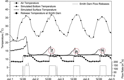
A similar process to the one described above was repeated for other large releases (Fig. 11). For example, for the release on 3 June, well-mixed temperature occurred at 14:45 h, which corresponded to the flow increase at 13:00 h (Fig. 11). Without large releases for more than 2 days before 1 June, surface temperature reached a maximum value of 23.6°C, and with a large release each day after 1 June, the maximum surface temperatures at MSF only reached 16.2–17.7°C. After a few hours of heating, maximum temperature differences at MSF reached 3–5°C before the stratification was removed by the next release. Both surface and bottom water temperatures at MSF increased with time over 1–2 h due to solar heating (circled by three red circles in Fig. 11) after complete mixing occurred, and then decreased with time to about 12.5°C.

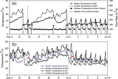
Time series of modeled surface and bottom temperatures at MSF from 21 May to 10 June (Fig. 12(a)) show the comparison of temperature variations at MSF with and without daily large releases from Smith Dam. From 21 May to 31 May there were four irregular large releases from Smith Dam that resulted in strong stratification between surface and bottom layers during day and night at MSF. The maximum temperature difference between surface and bottom layers was up to 5.9°C on 26–29 May 2011. Bottom temperatures at MSF steadily increased from ~13.0 to ~18.0°C for the periods of 21–23 May, 26–29 May (13.9–17.9°C) and 31 May–1 June. Although small constant release had a lower temperature of ~8.5°C (Fig. 12), the release of 2.83 m³/s could not overcome the temperature increases in Sipsey Fork due to solar heating. Surface temperatures at MSF increased with time with a few degrees of diurnal variations and maximum surface temperature reached 23.8°C. When a large flow release from Smith Dam occurred at 14:00 h on 23 May (lasting for 6 hrs), the large flow momentum completely mixed released water with warmer water in Sipsey Fork and caused the higher surface temperature to decrease and the lower bottom temperature to increase (Figs 11 and 12). Three releases on 23–25 May resulted in bottom temperatures at MSF of about 12.5°C (Fig. 12). There was a short release starting at 20:00 h on 29 May lasting for only 1 hr (Fig. 12). As a result of this 1-h release, bottom temperatures at MSF dropped from 19.8°C (after more or less completely mixing) to 13.5°C over a 24-h period, but surface temperatures at MSF started to increase after 05:00 h on 30 May. From 23 May to 1 June, the maximum and average temperature differences between surface and bottom layers were 7.1 and 4.4°C excluding well-mixed periods resulting from four irregular large releases. With daily regular releases from 1 June to 9 June (Fig. 12(a)), the maximum and average temperature differences between surface and bottom layers were 5.3 and 2.4°C (excluding well-mixed periods). Figure 12(a) clearly shows regular daily large releases did maintain relatively lower water temperatures at the bottom layers that promoted the density current formation further downstream of Sipsey Fork, but solar heating resulted in water temperature increases at the surface layer before the next large release.

Figure 12. Time-series of modeled surface and bottom temperatures at the middle of Sipsey Fork, upstream of the junction and downstream of the junction from May 22 to 11 June 2011 including release flow and temperature measured at Smith tailrace.

4.4 Temperature variations at UPJ and MJC

Figure 12(b) shows simulated surface and bottom temperatures at UPJ and MJC (Fig. 1). Surface temperatures at UPJ and MJC had distinct diurnal variations (Fig. 12(b)). From 21 May to 1 June, the maximum and average temperature differences between surface and bottom layers at UPJ were 9.7 and 4.4°C. During these 11 days, about 77% of the time, there were temperature differences greater than 0.5°C and 23% of the time with well-mixed conditions resulted from four irregular large releases. With daily regular releases from 1 June to 9 June (Fig. 12(b)), the maximum and average temperature differences between surface and bottom layers at UPJ were 10.7 and 3.5°C (excluding well-mixed periods), but during these 8 days, only 30% of the time were there temperature differences greater than 0.5°C and 70% of the time with well-mixed conditions at UPJ.

In an attempt to closely examine the impact of each large release from Smith Dam on surface and bottom temperatures at downstream locations, Fig. 12(b) shows interesting information on the movement of well-mixed flows after the releases (see Fig. 10(b)). The large release on 23 May resulted in the well mixed conditions with sharp temperature drop at MSF and UPJ just a few hours after the release, but the same condition at MJC occurred around the middle of the night of 25 May. This block or trunk of well-mixed water took more than 24 hrs to travel from SDT to MJC (33 km distance). The same phenomenon occurred for the release on 1 June (indicated by two red arrows for these two situations).

The daily releases from Smith Dam on 2–10 June created the well-mixed conditions in MSF in a few hours and stratification occurred during the next day with higher temperatures due to the solar heating (Fig. 12(a)). These daily releases occurred about 1–2 hrs after noon, the well-mixed conditions then occurred in the same afternoon and during the night at UPJ, and thermal stratification occurred during the next day due to solar heating of surface waters (Fig. 12(b)). Bottom temperatures at MJC (blue line with triangles) are typically higher than bottom temperatures at other upstream locations (MSF and UPJ shown in Fig. 12), which means solar heating can penetrate and reach the deeper waters near the river bottom (Fig. 12(b)).

4.5 Temperature variations at Cordova

Figure 13(a) shows time-series of modeled surface and bottom temperatures at the USGS Cordova monitoring station including release flow (m³/s) from Smith Dam and other tributary flows from 11 April to 28 October 2011. It clearly shows how strong temperature stratification existed between surface and bottom temperatures at Cordova. It seems that temperature stratification was much larger when there was only small constant release from Smith Dam. During large rainfall events (15–31 April and 6–8 September), surface and bottom temperatures were completely mixed due to runoff and streamflow from tributaries and watersheds.

Figure 13. (a). Time-series of air temperature, modeled surface and bottom temperatures at the USGS Cordova monitoring station under actual releases and base flow only, tributary inflow, release flow (m³/s) from Smith Dam from April 11 to 28 October 2011. (b) Zoom in from May 21 to 10 June 2011 including modeled deep depth temperatures with base flow release (2.83 m³/s) from Smith Dam.

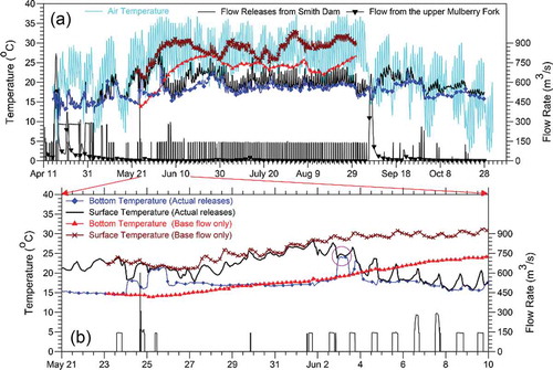
Figure 13(b) shows a detailed comparison of water temperatures from 21 May to 10 June 2011 to further illustrate simulated temperature stratification at Cordova. Simulated temperature stratification between surface and bottom layers at Cordova was up to 11.4°C with an average temperature difference of 1.53°C and standard deviation of 1.94°C under actual flow releases from Smith Dam. Twenty five percent (25%) of simulated surface and bottom temperatures at Cordova had temperature stratification less than 0.17°C from 11 April to 28 October 2011. The more or less completely mixed condition occurred around midnight of 3 June at Cordova (Fig. 13(b), pink circle) that was about 1.5 days after the release from Smith Dam on 1 June. The density current created from the flow release on 1 June seems to have travelled for about 36 hrs before it reached Cordova. The 1-h flow release which occurred on 29 May did show its impact in Sipsey Fork (Fig. 12(a)), but it showed no impact on temperature stratification at Cordova (Fig. 13).

Figure 13(b) shows that diurnal variations of surface temperature at Cordova were smaller (about a few degrees). Some sudden surface temperature decreases and bottom temperature increases shown in Fig. 13(b) were due to sudden flow releases from Smith Dam, as explained using Figs 10 and 11. These temperature decreases and increases at Cordova responded with two releases between 23 and 24 May in ~12 hrs, but responded with the releases between 1 and 2 June in more than 24 hrs. These different responses are not well understood yet; but they might be related to the strength of stratification at Cordova before each release.

Figure 13 also compares modeled surface and bottom temperatures at Cordova in 2011 under actual releases (constant release plus intermittent large releases) and assumed small constant or baseflow (2.83 m³/s) release only from Smith Dam. The simulation for baseflow only is from 23 May to 30 August 2011. It clearly shows that simulated bottom temperatures could keep on increasing before 25 June and surface temperatures are higher and follow with air temperature when there were no intermittent large releases from Smith Dam. Simulated maximum bottom temperature is 27.2°C under baseflow scenario and 24.3°C under actual releases, which occurred on 3 June (Fig. 13(b)) resulted from the large release on 1 June. Under the baseflow scenario, simulated average difference of surface and bottom temperatures is 8.0°C (50% of differences are greater than 5.3°C), but under actual releases, the average difference is 2.0°C (only 25% of differences are greater than 3.0°C), even though the maximum surface and bottom temperature differences for both cases are the same (11.4°C). Large releases on 23–25 May and 1–2 June actually resulted in higher bottom temperatures at Cordova when cooler bottom waters were completely mixed with warmer surface waters. Daily large releases starting from 1 June resulted in surface temperature decreases from 2 June (surface wave moving faster downstream) and bottom temperature decreases from 4 June (density currents at the bottom moving slowly downstream).

Statistical parameters for differences of surface or bottom temperatures simulated under the baseflow only and actual releases are summarized in Table 5 for five locations (MSF, UPJ, MJC, Cordova and GOUS) for the simulation period from 23 May to 30 August 2011. Bottom temperatures at Cordova and GOUS under the baseflow only are on average 4.81 and 4.26°C higher than bottom temperatures simulated under actual flow releases (baseflow plus intermittent large releases). Under the baseflow only scenario, simulated surface temperature at GOUS is up to 15.64°C higher than surface temperatures under actual releases from Smith Dam in 2011 (Table 5). Therefore, intermittent large releases significantly reduced surface and bottom temperatures in BRRS in comparison to the baseflow release.

Table 5. Statistics of differences of simulated temperatures (°C) at different locations from 23 May to 30 August, 2011, between under the baseflow only and using actual releases from Smith Dam.

Location	Maximum	Minimum	Average	Standard Deviation	25th percentile	Median	75th percentile
MSF (Bottom)	11.25	−3.58	7.05	1.68	6.26	7.16	8.05
MSF (Surface)	7.53	0.00	4.12	1.41	3.30	4.23	5.13
UPJ (Bottom)	12.71	−2.23	7.31	2.46	6.27	7.75	9.08
UPJ (Surface)	8.94	−0.04	3.52	1.37	2.55	3.48	4.41
MJC (Bottom)	13.13	−7.12	6.36	3.15	4.56	6.94	8.56
MJC (Surface)	9.65	−0.04	2.62	2.10	0.79	2.30	4.05
Cordova (Bottom)	9.78	−7.37	4.81	2.80	4.16	5.46	6.65
Cordova (Surface)	14.29	−0.34	7.95	3.31	5.75	8.72	10.47
GOUS (Bottom)	8.88	−2.44	4.26	2.33	3.69	4.75	5.64
GOUS (Surface)	15.64	4.62	10.52	1.94	9.58	10.72	11.70

4.6 Particle tracking on density current movement

In order to understand the propagation of density currents along the river bottom in BRRS, EFDC’s particle tracking method (Craig 2011) was used to trace the movement of density currents. One thousand particles were released in the middle depth layer at two locations: SDT and MJC (Fig. 1), at noon on 3 June (JD 153.5) when a large release from Smith Dam started. Particle counts in a 5-minute interval were reported in all grids over the cross-sections of MSF, UPJ, MJC, Cordova and GOUS, which give number of particles in defined control volumes (e.g. the volume at MSF covers about 90 m of Sipsey Fork). The 1000 particles released at Smith Dam first travelled and arrived at MSF, and 347 particles were reported at MSF at 15:35 h on 3 June. Because the 5-min interval was used to report particle count, the number of particles that passed through MSF between 15:30 and 15:35 h is unknown. Based on particle count distribution at MSF, average travel time for particles arriving at MSF was 3 hrs 40 min. Based on surface and bottom temperature distributions at MSF shown in Fig. 11, well-mixed conditions at MSF first occurred at 14:00 h (15-min reporting intervals). It seems that the momentum developed from the large release at noon on 3 June generated the movement and mixing of water at MSF before released water or particles actually reached MSF.

It was found that 90 particles reached UPJ at 22:35 h, which gave the travel time for these particles traveling through Sipsey Fork from SDT to UPJ (21.8 km). Four hundred and forty seven (447) particles reached MJC between 21:20 and 23:15 h on 4 June, which meant it took about 33 hrs for released water at SDT to travel BRR system and reach MJC (32.3 km travelling distance). First 54 particles reached Cordova monitoring station between 21:15–21:45 h on 5 June, hence it took more than 2 days (~57.5 hrs) for these particles to travel through Sipsey Fork and the lower Mulberry Fork to Cordova (43.6 km). A few particles showed at GOUS at 00:05 h (just after midnight) on 7 June and more particles showed up at 18:00 h on 7 June, which corresponds to more than 4 days for particles released on 3 June to reach GOUS.

For 1000 particles released from MJC at 12:00 h on 3 June, about 110 particles reached Cordova at 10:25–11:00 h on 4 June, and only 14 particles reached GOUS at 22:55–23:55 h on 7 June. The above preliminary results using particle tracking show that particles of water released from Smith Dam could take significant time to reach Cordova and GOUS but the momentum developed by the large releases affected downstream locations relatively shortly after the releases. This is further explained using Fig. 7 that gives cross-sectional average velocities at MSF, UPJ, MJC, Cordova and GOUS. After each daily large release around noon from 4–9 June, typically within 2 hrs after the releases velocities started to increase at all five locations, even Cordova and GOUS had velocity increases within 3 hrs after the releases. On 7 June, the large release at 15:00 h was more than 280 m³/s (Fig. 11(a)) and resulted in maximum velocities at MSF, UPJ, MJC, Cordova and GOUS of about 0.84, 0.67, 0.55, 0.24 and 0.24 m/s, respectively. The time of peak velocity occurred earlier at upstream locations and later at further downstream locations, but the time of peak velocity at GOUS occurred about 7 hrs after the release (not several days). Therefore, the momentum or push effect from the large release is the ultimate driving force for the density current movement at different locations along the river bottom in BRRS. Average velocities did attenuate to small magnitudes within 24 hrs at all cross-sections (Fig. 7), which indicates daily regular releases are necessary to promote the movement or advancement of the density current towards downstream.

5 Summary and conclusions

A three-dimensional hydrodynamic EFDC model was applied to simulate unsteady flow patterns and temperature distributions under various upstream releases and variable atmospheric forcing in BRRS. The calibrated EFDC model provided simulated water surface elevation, temperature, velocity and discharge at different layers (depths) for all grids in different cross-sections (Fig. 1). Overall, the EFDC model was able to predict the temporal and spatial distributions of flow and temperature (Fig. 10) and revealed complex interactions and density currents due to dynamic upstream releases and solar heating from the atmosphere. The major findings of the study are summarized as follows:

1. Simulated water depth, velocity and flow rate in Sipsey Fork increased first, then gradually and steadily decreased with time after the release from Smith Dam, and the recession lasted more than 12 hrs at MSF (Figs 6 and 7). After a few hours of heating, maximum temperature differences at MSF reached 3–5°C before the stratification was removed by the next release (Fig. 10). Simulation results clearly show that regular daily large releases did maintain relatively lower water temperatures at the bottom layers (Figs 12 and13) that promoted the density current formation further downstream of Sipsey Fork. Strong temperature stratification existed between surface and bottom temperatures at Cordova (e.g. 26–31 May, Fig. 13) without daily releases from Smith Dam. Simulated surface and bottom temperatures at Cordova kept on increasing first and then varied with air temperature trend when it was assumed that there were no intermittent large releases from Smith Dam.

2. The flow momentum created by the large release removed the thermal stratification at MSF. The well-mixed condition at MSF was developed 1.75 hrs after the release started. When there was a daily large flow release from Smith Dam, Cordova and GOUS responded with surface-layer flow rate changing from moving upstream (SDT) to moving downstream (BLD) roughly 2–3 hrs after the release. The flow rates moving downstream in the bottom layer had obvious increases. These daily releases promoted and enhanced the movement of density current moving from upstream towards downstream.

3. Preliminary results using particle tracking show that particles or water released from Smith Dam could take several days to reach Cordova and GOUS and the momentum developed by the releases did push the cooler water near the river bottom moving downstream. The momentum or push effect from the large release provides driving force for the density current movement along the river bottom in the BRR system.

Acknowledgements

The authors wish to express their thanks to Dr. William E. Garrett Jr., Mr. Jonathan B. Ponstein, P.E., and Mr. Tim George, P.E., for providing helpful comments and necessary data for the study. The authors would like to thank the Associate Editor and two anonymous reviewers for providing valuable comments and suggestions that helped us to improve the manuscript. The author Gang Chen wishes to express his gratitude to the Chinese Scholarship Council for financial support in pursuing his graduate study at Auburn University.

Disclosure statement

No potential conflict of interest was reported by the authors.

References

- Akiyama, J. and Stefan, H.G., 1984. Plunging flow into a reservoir: theory. Journal of Hydraulic Engineering ASCE, 110 (4), 484–499. doi:10.1061/(ASCE)0733-9429(1984)110:4(484)
- Alavian, V., 1986. Behavior of density currents on an incline. Journal of Hydraulic Engineering, 112 (1), 27–42. doi:10.1061/(ASCE)0733-9429(1986)112:1(27)
- Alavian, V. and Ostrowski Jr., P., 1992. Use of density current to modify thermal structure of TVA reservoirs. Journal of Hydraulic Engineering, 118 (5), 688–706. doi:10.1061/(ASCE)0733-9429(1992)118:5(688)
- An, S. and Julien, P.Y., 2014. Three-dimensional modeling of turbid density currents in Imha reservoir, South Korea. Journal of Hydraulic Engineering, 140, 5. doi:10.1061/(ASCE)HY.1943-7900.0000851
- Buchak, E. and Edinger, J., 1984. Simulation of a density underflow into Wellington Reservoir using longitudinal-vertical numerical hydrodynamics. Document. Vicksburg, MS: U.S. Army Corps of Engineers Waterways Experiment Station.
- Çalışkan, A. and Elçi, Ş., 2009. Effects of selective withdrawal on hydrodynamics of a stratified reservoir. Water Resources Management, 23 (7), 1257–1273. doi:10.1007/s11269-008-9325-x
- Carmack, E.C., et al., 1979. Importance of lake-river interaction on seasonal patterns in the general circulation of Kamloops Lake, British Columbia. Limnology and Oceanography, 24 (4), 634–644. doi:10.4319/lo.1979.24.4.0634
- Carron, J.C. and Rajaram, H., 2001. Impact of variable reservoir releases on management of downstream water temperatures. Water Resources Research, 37 (6), 1733–1743. doi:10.1029/2000WR900390
- Chikita, K., 1992. The role of sediment-laden underflows in lake sedimentation: glacier-fed Peyto Lake, Canada. Journal of the Faculty of Science, Hokkaido University. Series 7, Geophysics, 9 (2), 211–224.
- Cole, T.M. and Wells, S.A., 2010. CE-QUAL-W2: a two-dimensional, laerally averaged, hydrodynamic and water quality model, version 3.6 user manual. Instruction report EL-03-1. Vicksburg, MS: U.S. Army Engineering and Research Development Center.
- Consultants, 1986. Stanislaus project instream temperature study. In: Pacific gas and electric company. San Ramon, CA: Woodward-Clyde.
- Craig, P.M., 2010. User’s manual for EFDC_explorer: a pre/post processor for the environmental fluid dynamics code. Knoxville, TN: Dynamic Solutions, LLC.
- Craig, P.M., 2011. User’s manual for EFDC_explorer 6: a pre/post processor for the environmental fluid dynamics code. Knoxville, TN: Dynamic Solutions, LLC.
- Dallimore, C.J., Imberger, J., and Ishikawa, T., 2001. Entrainment and turbulence in saline underflow in Lake Ogawara. Journal of Hydraulic Engineering, 127 (11), 937–948. doi:10.1061/(ASCE)0733-9429(2001)127:11(937)
- Denton, R., 1985. Density current inflows to run of the river reservoirs. In: Proceedings of the 21st IAHR (International Association Hydraulic Research) World Congress, Melbourne, 13–18 August 1985.
- Devkota, J. and Fang, X., 2015. Numerical simulation of flow dynamics in a tidal river under various upstream hydrologic conditions. Hydrological Sciences Journal, 60 (10), 1666–1689. doi:10.1080/02626667.2014.947989.
- Fang, X. and Stefan, H.G., 2000. Dependence of dilution of a plunging discharge over a sloping bottom on inflow conditions and bottom friction. Journal of Hydraulic Research, 38 (1), 15–25. doi:10.1080/00221680009498354
- Farrell, G.J. and Stefan, H.G., 1989. Two-layer analysis of a plunging density-current in a diverging horizontal channel. Journal of Hydraulic Research, 27 (1), 35–47. doi:10.1080/00221688909499242
- Fernandez, R.L. and Imberger, J., 2008a. Relative buoyancy dominates thermal-like flow interaction along an incline. Journal of Hydraulic Engineering, 134 (5), 636–643. doi:10.1061/(ASCE)0733-9429(2008)134:5(636)
- Fernandez, R.L. and Imberger, J., 2008b. Time-varying underflow into a continuous stratification with bottom slope. Journal of Hydraulic Engineering, 134 (9), 1191–1198. doi:10.1061/(ASCE)0733-9429(2008)134:9(1191)
- Firoozabadi, B., Afshin, H., and Aram, E., 2009. Three-dimensional modeling of density current in a straight channel. Journal of Hydraulic Engineering, 135 (5), 393–402. doi:10.1061/(ASCE)HY.1943-7900.0000026
- Fischer, H.B. and Smith, R.D., 1983. Observations of transport to surface waters from a plunging inflow to Lake Mead [Nevada]. Limnology and Oceanography, 28, 258–272. doi:10.4319/lo.1983.28.2.0258
- Gu, R.R., 2009. Impact of inflow and ambient conditions on density-induced current in a stratified reservoir. Modern Physics Letters B, 23 (3), 429–432. doi:10.1142/S0217984909018576
- Hallworth, M.A., et al., 1996. Entrainment into two-dimensional and axisymmetric turbulent gravity currents. Journal of Fluid Mechanics, 308 (1), 289–311. doi:10.1017/S0022112096001486
- Hamrick, J.M., 1992. A three-dimensional environmental fluid dynamics computer code: theoretical and computational aspects. Gloucester Point, VA: The College of William and Mary, Virginia Institute of Marine Science.
- Hamrick, J.M. and Mills, W.B., 2000. Analysis of water temperatures in Conowingo pond as influenced by the Peach Bottom atomic power plant thermal discharge. Environmental Science & Policy, 3 (Supplement 1), 197–209. doi:10.1016/S1462-9011(00)00053-8
- Hauenstein, W. and Dracos, T., 1984. Investigation of plunging density currents generated by inflows in lakes. Journal of Hydraulic Research, 22 (3), 157–179. doi:10.1080/00221688409499404
- Imberger, J. and Patterson, J., 1980. Dynamic reservoir simulation model- DYRESM: 5. In: Proceedings of a symposium on predictive ability, 18–20 August 1980, Berkeley, CA. New York: Academic Press, 310–361.
- Imran, J., et al., 2007. Helical flow couplets in submarine gravity underflows. Geology, 35 (7), 659–662. doi:10.1130/G23780A.1
- Jeong, S., et al., 2010. Salinity intrusion characteristics analysis using EFDC model in the downstream of Geum River. Journal of Environmental Sciences, 22 (6), 934–939. doi:10.1016/S1001-0742(09)60201-1
- Jokela, J. and Patterson, J., 1985. Quasi-two-dimensional modelling of reservoir inflow. ed. Preprinted proceedings: 21st congress, international association for hydraulic research, 19–23 August 1985 Melbourne. Volume 2. Theme B(Part 1): Fundamentals and computation of 2-D and 3-D flows, 317–322.
- Kim, C.-K. and Park, K., 2012. A modeling study of water and salt exchange for a micro-tidal, stratified northern Gulf of Mexico estuary. Journal of Marine Systems, 96–97, 103–115. doi:10.1016/j.jmarsys.2012.02.008
- Kim, D., et al., 2009. VMS ADCP velocity mapping software. US Army Corps of Engineers, Vicksburg, MS 39180: Coastal & Hydraulics Laboratory, Engineer Research and Development Center.
- Kranenburg, C., 1993. Gravity current fronts advancing into horizontal ambient flow. Journal of Hydraulic Engineering, 119 (3), 369–379. doi:10.1061/(ASCE)0733-9429(1993)119:3(369)
- Kulis, P. and Hodges, B.R., 2006. Modeling gravity currents in shallow bays using a sigma coordinate model. In: The 7th international conference on hydroscience and engineering, 10–13 September, Philadelphia, PA.
- Liu, X. and Garcia, M.H., 2008. Numerical simulation of density current in Chicago river using Environmental Fluid Dynamics Code (EFDC). ed. Ahupua’a proceedings of the world environmental and water resources congress, 229 pp.
- Mellor, G.L. and Yamada, T., 1982. Development of a turbulence closure model for geophysical fluid problems. Reviews of Geophysics and Space Physics, 20 (4), 851–875. doi:10.1029/RG020i004p00851
- Petts, G.E., 1984. Impounded rivers: perspectives for ecological management. San Francisco, CA: John Wiley & Sons, 329 pp.
- Petts, G.E., et al., 1985. Wave-movement and water-quality variations during a controlled release from Kielder Reservoir, North Tyne River, UK. Journal of Hydrology, 80 (3–4), 371–389. doi:10.1016/0022-1694(85)90129-5
- Rueda, F.J. and MacIntyre, S., 2010. Modelling the fate and transport of negatively buoyant storm–river water in small multi-basin lakes. Environmental Modelling & Software, 25 (1), 146–157. doi:10.1016/j.envsoft.2009.07.002
- Savage, S. and Brimberg, J., 1975. Analysis of plunging phenomena in water reservoirs. Journal of Hydraulic Research, 13 (2), 187–205. doi:10.1080/00221687509499713
- Serruya, S., 1974. The mixing patterns of the Jordan River in Lake Kinneret. Limnology and Oceanography, 19 (2), 175–181. doi:10.4319/lo.1974.19.2.0175
- Shen, J. and Lin, J., 2006. Modeling study of the influences of tide and stratification on age of water in the tidal James River. Estuarine, Coastal and Shelf Science, 68 (1–2), 101–112. doi:10.1016/j.ecss.2006.01.014
- Singh, B. and Shah, C., 1971. Plunging phenomenon of density currents in reservoirs. La Houille Blanche, 1, 59–64. doi:10.1051/lhb/1971005
- Smagorinsky, J., 1963. General circulation experiments with the primitive equations. Monthly Weather Review, 91 (3), 99–164. doi:10.1175/1520-0493(1963)091<0099:GCEWTP>2.3.CO;2
- Smith, P.C., 1975. A streamtube model for bottom boundary currents in the ocean. ed. Deep sea research and oceanographic abstracts, 853–873.
- Toffolon, M., Siviglia, A., and Zolezzi, G., 2010. Thermal wave dynamics in rivers affected by hydropeaking. Water Resources Research, 46, W08536. doi:10.1029/2009WR008234
- Wang, Y., Shen, J., and He, Q., 2010. A numerical model study of the transport timescale and change of estuarine circulation due to waterway constructions in the Changjiang estuary, China. Journal of Marine Systems, 82 (3), 154–170. doi:10.1016/j.jmarsys.2010.04.012
- Weems, T.B., 2013. Water balance analysis using WARMF in support of an EFDC hydrodynamic Model. ( M.S.). Auburn University.
- Wunderlich, W.O. and Shiao, M.C., 1984. Long-range reservoir outflow temperature planning. Journal of Water Resources Planning and Management, 110 (3), 285–295. doi:10.1061/(ASCE)0733-9496(1984)110:3(285)