Review of the Kalman-type hydrological data assimilation

ABSTRACT

There is great potential in Data Assimilation (DA) for the purposes of uncertainty identification, reduction and real-time correction of hydrological models. This paper reviews the latest developments in Kalman filters (KFs), particularly the Extended KF (EKF) and the Ensemble KF (EnKF) in hydrological DA. The hydrological DA targets, methodologies and their applicability are examined. The recent applications of the EKF and EnKF in hydrological DA are summarized and assessed critically. Furthermore, this review highlights the existing challenges in the implementation of the EKF and EnKF, especially error determination and joint parameter estimation. A detailed review of these issues would benefit not only the Kalman-type DA but also provide an important reference to other hydrological DA types.

Editor D. Koutsoyiannis; Associate editor F. Pappenberger

KEYWORDS:

• data assimilation
• extended Kalman filter
• ensemble Kalman filter
• model error
• parameter estimation

1 Introduction

In the past few decades, hydrological models have significantly benefited from the improvement of computational capacity and the availability of multi-source measurement data to simulate and forecast hydrological processes. However, due to the deepening involvement of uncertainties stemming from initial conditions, inputs and outputs, operational hydrological models will remain inherently imprecise.

Data assimilation (DA) is a procedure developed to optimally merge information from model simulations and independent observations with appropriate modelling (Liu et al. 2012b). The DA could provide optimized initial conditions, updated parameters and even improved structures for the dynamic model. Originally used in areas such as atmospheric and oceanographic science (Derber and Rosati 1989, Dee 1995), DA has drawn the attention of hydrologists more and more for its convincing performance in the real-time correction of hydrological models (Robinson and Lermusiaux 2000).

Walker and Houser (2005) and Reichle (2008) summarized the basic hydrological DA methods; Moradkhani (2008) reviewed remote-sensing measurement techniques and their applications in DA; Liu and Gupta (2007) discussed the role of DA in addressing the uncertainties in hydrological models and discussed the application of the hydrological DA in operational scenarios (Liu et al. 2012b). Montzka et al. (2012) examined the joint assimilation of observational data precedents from different spatial scales and different data types. Reviews that focus on a specific method are relatively rare compared to reviews with a wide scope (e.g. Van Leeuwen 2009).

The Kalman filter (KF) is a classic sequential method that has been widely used in hydrological DA for more than two decades (Evensen 1994b, McLaughlin 1995). Compared to other methods, such as particle filters (PFs) and variational methods, the KF is easier to implement and could produce comparable or even better results with a lower computation demand (Weerts and El Serafy 2006, Abaza et al. 2014b). Furthermore, the KF is very flexible for coupling with hydrological models and has more derivative variants than any other methods. Among these variants, the Extended KF (EKF) and the Ensemble KF (EnKF) were both developed to extend the application of the KF to nonlinear systems; also, they are the two major descendants of the linear KF. The EKF applies a straightforward Taylor extension scheme to linearize the nonlinear system. As logical as it is, the EKF has endured a “notorious” reputation for being unstable when applied to complex nonlinear hydrological models. The EnKF avoids direct linearization by statistically analysing the ensemble members. Although it increases the computational cost, the EnKF is one of the most widely used hydrological DA methods. Despite some comparison case studies (Reichle et al. 2002b, El Serafy and Mynett 2004, Dumedah and Coulibaly 2012), there is no critical review that specifically focuses on the KF. The objective of this review is to fill this gap by assessing the latest developments and analysing the challenges of Kalman-type hydrological DA, especially the EKF and EnKF. Nevertheless, this review is not intended to judge which method is better, but rather regards them as different solutions to the same problem. This is not only because they both branched from the linear KF, but also because they face some similar issues when applied in hydrological DA, of which some are also faced by methods other than KFs.

In the rest of the paper, we introduce hydrological DA, including the DA targets and methods in Section 2. The theory of the KF (including EKF and EnKF) and its state of the art applications in hydrological DA are discussed in Section 3. Section 4 discusses issues regarding the implementation of the KF in hydrological models. The summary and conclusions are given in Section 5.

2 Hydrological data assimilation

2.1 Hydrological DA targets

Data assimilation was first used in the 1950s for numerical weather forecast modelling; however, hydrologists did not pay much attention to it until the 1990s (Evensen 1994b, McLaughlin 1995). Proper use of DA may help in handling uncertainties from model inputs, the initialization and propagation of states, the model structures and even the model parameters (Vrugt et al. 2006, Liu and Gupta 2007, He et al. 2012). Meanwhile, global DA may improve regional field estimation by achieving more accurate external boundary condition estimations (Robinson and Lermusiaux 2000), and local DA could also lead to improved global estimations (Clark et al. 2008).

The development of remote sensing has promoted the application of DA in hydrological models. The remotely sensed hydrological data that have had, or currently have, the potential to be applied in hydrological models include (Houser et al. 2005, Walker and Houser 2005, Xu et al. 2014):

1. overland parameters (e.g. topography, land cover, albedo);

2. forcing inputs (e.g. precipitation, air humidity and temperature);

3. states (e.g. soil moisture, snow cover);

4. fluxes (e.g. carbon flux).

The overland parameters are usually regarded as “static” in the model, even though this is not true in long-term forecasts. Forcing inputs have the potential to replace traditional ground-based observations, with the development of remote-sensing instruments and more accurate retrieval algorithms. Neither overland parameters nor forcing inputs are the main interest of DA for hydrological modellers at this stage. The states and fluxes provide validation to the intermediate processes of the models. This was not available earlier, and hence has drawn extra attention.

Snow cover has a high albedo and thermal properties, as well as medium-term water storage capacity; therefore, the assimilation of snow observations could improve hydrological prediction (Walker et al. 2003). Andreadis and Lettenmaier (2006) used the EnKF to assimilate remotely sensed snow observation moderate resolution imaging spectroradiometer snow cover extent (MODIS SCE) data into the VIC hydrological model to update snow-water equivalent (SWE) estimates. From these estimates, a simple snow depletion curve scheme from SNOTEL station SWE data and MODIS imagery (Moradkhani 2008) was used to form the observation operator. Clark et al. (2006) assimilated the observations of a snow-covered area (SCA) to update the hydrological model, and they found that the assimilation of SCA information results in minor improvements in the accuracy of streamflow simulations near the end of the snowmelt season. Both of them found that the snow-cover update works better during the snowmelt season than the snow-accumulating season. Further research with regard to snow-cover assimilation can be found in the literature (Pan et al. 2003, Sheffield et al. 2003, Rodell and Houser 2004, Kumar et al. 2008, Parajka and Blöschl 2008).

Galantowicz et al. (1999) demonstrated KF retrieval of the soil moisture profile and temperature from L-band radio brightness observations, while Crow and Wood (2003) applied the EnKF to assimilate airborne measurements of surface brightness temperature into a TOPMODEL-based Land–Atmosphere Transfer Scheme (TOPLATS). Due to the short memory the land-surface skin temperature holds, it is suggested that it could be combined with other state variables with longer memories, such as deeper soil temperature or moisture, to obtain longer DA effectiveness (Walker et al. 2003). The surface temperature products are also sensitive to terrain, vegetation and cloud contamination; hence, multiple sets of products and better retrieval algorithms are required for continuous DA operations (Huang et al. 2008).

Soil moisture is the key variable to control the runoff generation process. It is logical to assimilate soil moisture directly, because it is a continuous storage indication as well as a natural bridge to transfer the hydrological model into state-space equations. The correct estimation of antecedent soil moisture content is critical to streamflow simulation when the soil is neither too dry nor over-saturated (Reichle et al. 2002a). Soil moisture assimilation has been proven beneficial to streamflow prediction, especially that for low flow. (Chen et al. 2014, Wanders et al. 2014b). The application of soil moisture requires the ground-based measurements to be dense enough (Chen et al. 2011), otherwise the spatial interpolation error will have to be considered. Satellite remote sensing can provide an economic and more spatial-temporal continuous observation of soil moisture.

Parrens et al. (2014) assimilated in situ soil moisture observations into a soil model at local scale. Reichle et al. (2002a) assimilated L-band microwave brightness temperature into a land surface model to estimate the near-surface soil moisture. Crow and Ryu (2009) used remotely sensed soil moisture retrievals to correct both the soil moisture state and satellite rainfall products. Alvarez-Garreton et al. (2014) assimilated surface soil moisture and soil wetness index derived from passive microwave Advanced Microwave Scanning Radiometer-Earth Observing System (AMSR-E). Brocca et al. (2012) assimilated surface and root-zone soil moisture products derived from the active microwave advanced scatterometer (ASCAT) into a rainfall–runoff (RR) model using the EnKF. Recently, soil moisture assimilation has also been used to assist the parameter identification of hydrological models (Tran et al. 2014, Wanders et al. 2014a).

Despite the existence of some root-zone soil moisture by-products from the surface soil moisture observations (Wagner et al. 1999, Das et al. 2008), one of the obvious drawbacks of remote sensing of soil moisture is that only surface or near-surface soil moisture is available (Moradkhani 2008, Han et al. 2012). Preliminary experiments showed that surface soil moisture assimilation has a minimal effect on the simulation of the deep-layer soil moisture (Chen et al. 2011), although it is the latter that has a more significant impact on runoff simulations (Brocca et al. 2012, Han et al. 2012). Houser et al. (1998) argued that the remotely sensed soil moisture must be supplemented by in situ surface and root-zone observations to specify error correlation, calibrate parameters, and validate the model-calculated fields. Draper et al. (2011) found that it might be more effective to address the cause of model bias instead of relying on soil moisture assimilation to correct it. Some research combined soil moisture assimilation with the correction of other RR model forcings, such as precipitation, to improve streamflow predictions (Chen et al. 2014, Massari et al. 2014). The application of remote sensing of soil moisture may also involve issues such as rescaling (Kaheil et al. 2008, Sahoo et al. 2013), error evaluation (Alvarez-Garreton et al. 2014, Doubková et al. 2012), and radiative transfer modelling (Verhoef and Bach 2003, Reichle 2008), among others. A more detailed explanation of the limitations of soil moisture assimilation can be found in the literature (Vereecken et al. 2015).

Streamflow is the most commonly used and sometimes the only available prognostic observation variable (Clark et al. 2008, Randrianasolo et al. 2014, Samuel et al. 2014, Trudel et al. 2014, Abaza et al. 2014a). Great efforts have been made to improve streamflow forecasting using output assimilation/error assimilation over the past two decades (Broersen 2007, Anctil et al. 2003, Yu and Chen 2005, Sene 2008). The output/error assimilation methods treat a streamflow forecast as a pure model output and update it by adding errors calculated with another independent procedure or model. Such procedures/models could either be nonlinear, such as artificial neural networks (ANNs; Anctil et al. 2003), or linear, such as autoregressive–moving-average models (Broersen 2007, Chen et al. 2015). Output/error assimilation of streamflow is relatively simple to implement, as there is no feedback to the original RR model from the manipulation of model outputs.

Besides being the direct assimilation goal (Liu et al. 2012a), streamflow is also the prevalent observation to assimilate other state variables and parameters (Coustau et al. 2013). In hydrological DA, streamflow is often treated as a diagnostic variable, and is therefore not updated directly (Clark et al. 2008). In the case of a nonlinear measurement operator, it is probably the only choice to augment the state vector with the streamflow (Evensen 2003). By doing so, the nonlinear measurement operator should be reduced to a linear matrix, otherwise one would have to linearize the measurement operator. Pauwels and De Lannoy (2009) attempted to linearize the nonlinear discharge–watershed storage relationship (observation operator) in a “brutal” way. Linearization was undertaken within both a simple time series model and a conceptual Hydrologiska Byråns Vattenbalansavdelning (HBV) model; the results showed that direct linearization should be bypassed to obtain a better assimilation result.

Streamflow assimilation is different from other state variables because it involves the issue of routing. When the runoff is assimilated into a hydrological model at the current time step, not only does the current state of the watershed at a given location (e.g. outlet) need to be updated and propagated forward, but also the state at a number of different locations at multiple previous time steps (Pauwels and De Lannoy 2006). This is the case especially concerning large and distributed hydrological models. Many authors actually choose not to go into the details of the complicated channel network to control the complexity of the problem (Weerts and El Serafy 2006, Clark et al. 2008).

Despite the unique challenges faced by these targets, they share some common issues in their implementation, most notably in the quantification of observation errors and the determination of observation operators that connect them with the model output (Andreadis and Lettenmaier 2006). It is also worth pointing out that the assimilation of one single variable does not necessarily improve the estimation of the other variables. Trudel et al. (2014) reported that the assimilation of the streamflow at the outlet of the watershed would distort the estimate of soil moisture. A combination of multiple observation variables seems to be superior to single variable assimilation (Xie and Zhang 2010, Trudel et al. 2014).

The last decade saw the development of various global and regional land assimilation systems (Cosgrove et al. 2003, Mitchell et al. 2004, Rodell et al. 2004, Kumar et al. 2008). These systems enable the incorporation of multi-source observations, multi-models and multi-assimilation schemes in creating an optimal land surface states output. Due to possible water and energy balance issues, a major concern in land assimilation systems is whether they should be coupled to atmospheric models (Walker et al. 2003). Betts et al. (2003) compared the water budget of European Center for Medium range Weather Forecasting (ECMWF) 40-year reanalysis and NASA (National Aeronautics and Space Administration) DAO (Data Assimilation Office) fvGCM (finite-volume general circulation model) with the hydrological balance of the VIC model and the radiative fluxes with basin averages derived from International Satellite Cloud Climatology Project (ISCCP). They found that the runoff from both atmospheric models was significantly underestimated compared to the VIC runoff simulation, which is consistent with the observed streamflow. Large bias is also observed for radiation fluxes and surface temperature between ECMWF 40, fvGCM and the ISCCP data. Pan and Wood (2006) suggested a constrained EnKF to maintain the benefit of DA without violating the water balance principle. Boulet et al. (2000) and Bøgh et al. (2004) developed a simple water and energy balance model that allows the direct application of the remote-sensing data.

2.2 DA methods

The DA methods can be divided into different categories based on different standards (Rakovec et al. 2015). According to the dimension they focus on, these approaches can be classified as objective analysis methods and time-dependent methods (Wang and Kou 2009).

2.2.1 Objective analysis

Objective analysis aims to minimize the error between the observation field and the background field (usually the output of the numerical models) by “fusing” the new observations into the background with spatial dimensions. Typical objective analysis methods include successive correction (Cressman 1959, Barnes 1964), optimal correction (Gandin 1965, Lorenc 1981), statistical bias correction (Piani et al. 2010), Newtonian nudging (Houser et al. 1998, Paniconi et al. 2003), variational methods (Reichle et al. 2001, Seo et al. 2003, 2009, Navon 2009), etc. Detailed descriptions about the theory and development of the above methods can be found in the literature (Navon 2009).

Since objective analysis methods mostly take “snapshots” of the background filed at a given time (McLaughlin 1995), the temporal dimension is usually not well incorporated with the spatial dimensions. Even though some of them do consider the temporal dimension, such as 4-dimensional variational (4D VAR) and Newtonian nudging, time-variant objective methods are most simply viewed as a dynamic extension of the time-invariant version of the objective methods (McLaughlin 2002).

Among various objective analysis methods, the successive correction and nudging methods fail to consider the errors in the observations, while 3-dimensional variational (3D VAR) and 4D VAR ignore the uncertainties in the models. Objective analysis methods usually involve huge computations (Clark et al. 2008). Houser et al. (2005) suggested that the adjoints should be calculated as the model is developed, but this is by no means an easy task for distributed hydrological models.

2.2.2 Time-dependent methods

Time-dependent methods use a probabilistic framework and estimate the system state sequentially by propagating information forward in time (Bertino et al. 2003). The strength of the time-dependent methods is in time series analysis. The time-dependent methods work on a fixed but moving time window, and only the most recent observations that fall into this window are incorporated into the final estimation results. Typical time-dependent methods that are frequently used in hydrological DA include the linear KF (Kalman 1960) and its variants, such as the Extended KF (EKF) (Puente and Bras 1987), the Ensemble KF (EnKF) (Evensen 1994b), the Unscented KF (UKF) (Wan and Van Der Merwe 2000), the PF (Pham 2001, Moradkhani et al. 2005a, Weerts and El Serafy 2006), and the H-infinity filter (Moradkhani et al. 2005a, Wang and Cai 2008, Lü et al. 2010), among others. There are also some alternative approaches to solving specific issues in hydrological DA, most notably in the application of a genetic algorithm (GA) in the estimate of pixel-based soil hydraulic parameters for hydroclimatic modelling (Ines and Mohanty 2008) and evolutionary-based assimilation in streamflow simulations in ungauged watersheds (Dumedah and Coulibaly 2012). The spatial variation of the relationship between the background field and observation field of the variable in question is of less concern in time-dependent methods. Meanwhile, time-dependent methods are capable of handling more uncertainties (Moradkhani 2008) and are less complex to implement compared to some objective analysis methods that require an inverse or a joint model (Bertino et al. 2003).

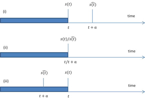
Time-dependent methods can be well explained with Wiener–Kolmogorov estimation theory (Kolmogorov et al. 1941, Wiener 1949). Suppose is the original signal, and is the estimated signal; the estimation error is defined as: where α is the delay of the estimation. In other words, the error is the difference between the estimated signal and the true signal shifted by α. Depending on the value of α, the estimation problem can be described as in Figure 1:

1. if α > 0, the estimation is a prediction problem (error is reduced when is similar to a later value of s(t));

2. if α = 0, the estimation is a filtering problem (error is reduced when is similar to s(t));

3. if α < 0, the estimation is a smoothing problem (error is reduced when is similar to an earlier value of s(t)).

Figure 1. Types of estimation problem: (i) prediction, (ii) filtering, (iii) smoothing.

In a broad sense, both smoothing and filtering are time-dependent DA methods as they both combine the advantages of measurements and model outputs. In a narrower sense, only filtering problems count as time-dependent DA methods, as DA only deals with “real-time” measurements instead of historical ones. In the case that the information in the time series is only propagated forward without any backward loop or window, the time-dependent methods are also termed sequential methods. The prediction problems usually serve as the validation of the smoothing and filtering problems. Traditional batch calibration technologies for hydrological models can be categorized as a smoothing problem (McLaughlin 2002). Filtering technologies usually play an important role in improving the prediction from the calibration; hence, they are widely used in real-time modules of operational models (Divac et al. 2009, McMillan et al. 2013).

2.2.3 Applicability of DA methods to hydrological models

Many approaches have been applied in hydrological DA (Houser et al. 2005, Walker and Houser 2005). The most commonly used methods include the variational method, PFs and the KFs. Although traditionally dominant in numerical weather forecasts, variational methods have not been widely used in hydrological DA. Variational methods such as 3D VAR assume the forecast error statistics are isotropic and largely homogeneous with little variation in time (Houtekamer and Mitchell 1998), though the consideration of the time dimension would overwhelmingly increase the computation burden. It is also complicated to develop the adjoint model for the distributed hydrological models (Clark et al. 2008). Successful cases using variational methods in hydrological DA are mostly based on simpler lumped models (Seo et al. 2003, 2009, Abaza et al. 2014b). Abaza et al. (2014b) compared the classic variational method with EnKF, and they found that the latter is more stable in streamflow assimilation.

PFs are also widely used in hydrology DA (Pham 2001, Moradkhani et al. 2005a, Weerts and El Serafy 2006). One of the major advantages of PFs is that the system does not need to be Gaussian (Liu et al. 2012b). PFs are also better at handling model nonlinearities compared to other sequential methods (Moradkhani et al. 2005a). The fact that PFs use full prior density means this method is more computationally intensive (Weerts and El Serafy 2006). The operational applications of PFs in distributed hydrological models are also limited due to the set-up of the particle numbers (Liu et al. 2012b).

Despite the thriving development of DA methods in “interpolation”, “smoothing” or “filtering”, not many of them are actually extensively validated in “forecast” mode, not to mention in operational hydrological forecasts (Liu et al. 2012b). One of the problems that hydrological DA faces is the short “efficient period”. The updating of model structures and storages generally has a major impact on the forecast only within shorter lead times (El Serafy and Mynett 2004, Knight and Shamseldin 2006). A possible reason for this is that DA deals with uncertainties from different data sources in a statistical way, rather than in a physical or mechanical way (McLaughlin 2002). It somehow “detours” the imperfect model structure and parameters in hydrological models by adding more weight to the model uncertainties, thereby emphasizing observations in the final results.

Numerical Weather Prediction (NWP) is fundamentally an initial problem that is very sensitive to state variation versus the hydrological models, which lean toward a process problem that relies on model structures and parameters. For this reason, DA might not work as well in hydrology as in NWP. However, because of the “conceptual” nature of most hydrological models, DA does have the potential to improve the model forecast either by updating the initial condition or modifying the model parameters.

A potential development direction of hydrological DA is the combination of objective analysis methods and sequential methods. 4D VAR expands the strength of 3D VAR by considering the temporal evolution of variables within the fixed time window. However, depending on the model structure, it could be expensive to calculate the gradients of the cost function (Bin and Ying 2005). The methods that combine the merits of both objective analysis and sequential methods, such as 4D VAR and EnKF, are generally regarded as the most promising DA technology in NWP (Lorenc 2003, Kalnay et al. 2007). However, as far as the authors are aware, such a dominant DA method still does not exist in operational hydrological simulation and forecasting.

3 EKF and EnKF

The linear KF is a classic sequential method. Together with its multiple nonlinear variants, such as the EKF and EnKF, the KF has become a very promising method cluster used in hydrological DA.

3.1 Linear KF

The KF is an optimal estimator that recursively couples the most recent measurements into the linear model to update the model state output (Kalman 1960). Under the assumption that the linear system is a stochastic process with Gaussian noise, the KF produces the best estimation with minimum mean square error.

The KF works on a stochastic system in the form of state space equations (Hamilton 1994):

(1)

(2)

Equation (1) is the model function that propagates state x from step k to step k + 1. x_k is the a posteriori state vector and x_k+1 is the a priori state. M_k is the model function (also known as the dynamic function or dynamic operator). B_k is a linear matrix to convert the dimension of residual vector u_k to state vector x_k. u_k is the “forcing” term of the model in the form of linear residuals. ŋ_k is the model estimation error (covariance matrix ). Sometimes, to simplify the problem, u_k is regarded as part of M_k and its estimation error is included in ŋ_k, and in this case B_k = 0.

Equation (2) is the observation function that relates the state vector x_k to the observation , with observation error ε_k (covariance matrix ). To guarantee the linearity of the system, the observation operator H_k should be linear too. Normally, the number of observation variables is limited while the state variable combinations could be infinite. It is probable that the observation vector dimension (degree of freedom) is much smaller than that of the state vector.

A typical implementation of the KF is described below (Drécourt 2003). At time step 0, set up the initial estimation error covariance matrix of the initial state . The model propagation without an explicit form for u_k is given by:

(3)

(4)

The superscript “a” represents a posteriori estimation and the superscript “f” means a priori estimation.

The state is then updated via:

(5)

where is the innovation and the Kalman gain is calculated with:

(6)

The estimation error is finally updated as:

(7)

With the updated estimation error, the filter can restart from Equations (3) and (4) to begin another loop recursively.

Equation (5) shows that the updated state is a linear combination of the observation and the model estimate (Drécourt 2003). The gain would change between 0 and H⁻¹ depending on the uncertainty comparison between the model outputs and the observations. For example, if the dynamic model is 100% accurate (which is unrealistic), then the new observation would not be considered at all in the updated state, as the gain is 0, and vice versa.

The linear KF tends to be more commonly used in stochastic models (Bolzern et al. 1980, Bergman and Delleur 1985, Szöllősi-Nagy and Mekis 1988) and channel routing problems (Huang 1999), which are easier to linearize (Georgakakos and Bras 1982, Fan 1991, Wu et al. 2008, Sun et al. 2013). However, there are a few successful cases in which the linear KF was applied in complex RR models. Liu et al. (2011) and Lee and Singh (1999) coupled a tank model with a linear KF to estimate the model parameter and outflow respectively. Kim et al. (2005) applied the KF in a one-dimensional physically based distributed model CDRMV3 with the storage amount of the whole watershed as state and outlet discharge as measurement, while a discharge–storage (Q-S) curve was used as the observation equation, in addition to a Monte Carlo ensemble being used as the dynamic equation. The drawback of such operations is that it could be difficult to find the linear relationship between discharge and storage, even at local scale.

3.2 Nonlinear KF

The KF is only legitimate in a linear system where both the model function M_k and the observation function H_k are linear. In the case of a nonlinear system (Drécourt 2003):

(8)

(9)

where is the model function and is the observation function, the linear KF is not applicable even if only one of them is nonlinear.

The hydrological system is a highly complicated nonlinear system with gigantic dimensions. In cases such as stochastic black-box streamflow prediction models, a linear KF might apply. However, it is not feasible to count on a linear KF in DA of distributed/semi-distributed hydrological models.

To cope with the nonlinear problem, many different versions of modified KFs have been developed (Shamir et al. 2010, Muluye 2011, Dumedah and Coulibaly 2012, Chen et al. 2013, de Rosnay et al. 2013, Gharamti and Hoteit 2014, Rakovec et al. 2015). A large portion of these booming new methods or algorithms are based on the EKF and EnKF.

3.2.1 EKF

3.2.1.1 Theory of the EKF

A prerequisite to applying the EKF is that the nonlinear system should be continuously differentiable. Under this condition, Taylor extension is applied at the estimated point. It is therefore possible to obtain the converted linear dynamic matrix by expanding the nonlinear functions at the estimated point. Apply this to both model function and observation function to get Equations (10) and (11) (Walker and Houser 2005):

(10)

(11)

The linearized and are then used in the calculation of error covariance propagation; all subsequent steps are the same as in the linear KF (Lewis et al. 2008). The EKF may be applied to the latest observation back and forth as many times as needed to reduce the linearization errors. However, such recursive operations do not guarantee a better estimation than the one-time EKF, while the computation burden is increased greatly (Puente and Bras 1987).

In many cases, nonlinear systems do not have explicit analytical solutions and the derivatives can only be calculated numerically. As the state is a vector with multiple variables, the linearized matrix can be expressed as a Jacobian matrix of the partial differential functions.

The EKF keeps the first order of the Taylor expansion, while it ignores the higher-order terms. Theoretically, a high-order EKF that keeps more than the first-order terms is more precise, as more information is kept (Tanizaki 1996, Simon 2006). However, it would still be biased because higher-orders terms are still ignored (Tanizaki 1996). In reality, there are rare cases supporting the superiority of higher-order EKF over first-order EKF (Sadeghi and Moshiri 2007, Ermolaev and Volynsky 2014). This is especially true when the analytical solutions of the system are unavailable, because the simultaneous numerical solution of the Jacobian and Hessian matrix may introduce more errors (Roth and Gustafsson 2011, Vittaldev et al. 2012).

3.2.1.2 Application of the EKF

The EKF has been widely used in operational soil moisture analysis by various weather agencies (Hess 2001, de Rosnay et al. 2013, Fairbairn et al. 2014). de Rosnay et al. (2013) described the operational implementation of a simplified EKF (SEKF; Draper et al. 2009, Mahfouf et al. 2009), in which the EKF has been simplified by setting constant background errors in the ECMWF land surface analysis system. The SEKF linearizes the observation operator with finite differences by adding individual perturbations to each element of the model state vector. Such a feature significantly increases the computation cost with the increase of dynamic model resolution. To solve this problem, one should either modify the model structure or calculate the Jacobian matrix from an off-line land surface model simulation (Mahfouf et al. 2009). The comparison between the SEKF and EnKF shows that the SEKF gives similar performance to EnKF; the latter is unable to improve on the former (Fairbairn et al. 2014).

Ge (1984) applied the EKF on a three-layer storage excess runoff model. Depending on the existence of precipitation and the fulfilment of each soil layer, they set 10 different runoff-generation scenarios. To avoid defining a threshold function, each scenario was assigned a state space function. By doing so, it is found that only two state space functions need to be linearized. Taylor expansion was then used with these two functions analytically. The constants from truncation of the Taylor expansion are treated as the linear driven terms of the model function and linear residuals of the observation function, respectively. Neither of them is involved in the state error propagation explicitly, but they are the integral components of the model and observation functions and cannot be neglected.

Kitanidis and Bras (1980a) linearized the Sacramento model using statistical linearization and a “describing function” technique. Instead of linearizing the nonlinear formulas directly, a group of simple linear functions that produce similar outputs with the same inputs as the nonlinear formulas are applied. The focus is thus shifted to the determination of the coefficients of the linear functions using statistical methods. This scheme is somehow “subjective”, because the candidate linear functions are not uniquely dependent on the selection criteria, or the evaluation functions to assess the fitness of the linear functions. Another challenge for this scheme is that it assumes that the inputs follow a constrained Gaussian distribution and, most importantly, they should fall in a very narrow range for the linear function replacement. The computation burden of statistical linearization is also a big issue.

Instead of implementing analytical linearization, Walker and Houser (2001) numerically derived the dynamic transition matrix in the propagation of the estimation error covariance. The state vector contains three intermediate soil moisture parameters and the forecast equations of state were linearized with a first-order Taylor series expansion. The observation chosen is the remote-sensing surface soil moisture, which is related to the state vector through a complicated nonlinear equation that is also linearized with a Taylor expansion. The numerical solution significantly increases the computation cost, but not as much as statistical linearization (Kitanidis and Bras 1980b). Therefore, it is important to provide a state vector of a manageable size. The problem with the numerical solution is the determination of the perturbation of the independent variables: small perturbations may lead to numerical problems, while large perturbations will cause a much greater loss of accuracy, and could also risk hitting the nonlinear threshold (Reichle et al. 2002b).

3.2.1.3 Assessment of EKF

The robustness issue of the EKF is well discussed in hydrological DA, and much of this concerns the divergence problem (Ljung 1979). The divergence of the EKF can be due to a number of reasons (Fitzgerald 1971): The first factor concerns the inappropriate estimation of the model and observation error covariance matrix, which will be discussed extensively in Section 4.2. Secondly, divergence can also be caused by the incorrect estimation of the initial estimation error P. Since the estimation of P at time k relies on P at time k − 1, a large error in initial P could recursively propagate until there is a divergence of the EKF (Tao et al. 2005). The third reason concerns the truncation errors arising from the Taylor expansion: although first-order local linearization is adequate to account for differential nonlinearity in some models (Reichle et al. 2002b), the existence of such errors makes it harder for the model errors to meet the whiteness assumption. Lastly, the errors from the numerical calculation of the Jacobian matrix: the perturbation scale of the independent variables involves subjective trials.

Many efforts have been made to alleviate the divergence of the EKF. Adaptive algorithms (Jwo and Wang 2007) are widely used to prevent the divergence caused by inappropriate error quantifications. Ljung (1979) introduced an innovation model by adding a parameterized Kalman gain term to the original EKF state space equations; he argued that the main reason for the divergence is the lack of coupling between Kalman gain K and model parameters. Tao et al. (2005) rescale the error covariance matrix by multiplying it by a factor; once the divergence is detected, the Kalman gain is frozen until stability is restored.

Compared to other nonlinear methods, the implementation of the EKF is direct and straightforward. It is arguably the de facto standard method to expand the KF to nonlinear systems for its outstanding performance in practice (Rabier and Liu 2003). However, it is not clear if the EKF can outperform other DA methods in nonlinear distributed hydrological models when considering the computational burden of linearization, even though strategies such as low-rank SEEK (singular evolutive extended Kalman; Tuan Pham et al. 1998) can reduce the computational requirements of the EKF.

3.2.2 EnKF

3.2.2.1 Theory of the EnKF

The EnKF is a Monte Carlo approach for nonlinear filtering problems (Evensen 1994a). There are two types of EnKF (Kalnay et al. 2007): perturbed observation EnKF (Evensen 1994b, Burgers et al. 1998) and square-root EnKF (Anderson 2001, Bishop et al. 2001, Whitaker and Hamill 2002). The perturbation of the observations causes additional sampling errors (Kalnay et al. 2007), but this type of EnKF could handle nonlinearities better than the square-root EnKF (Lawson and Hansen 2004).

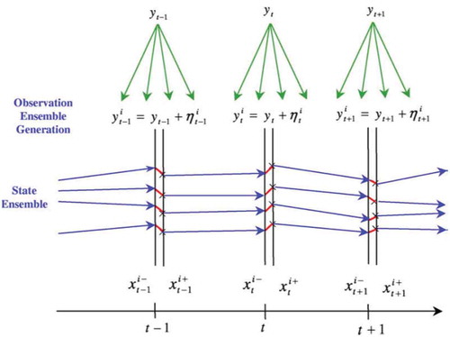
The EnKF is based on approximation of the conditional probability densities of the state error covariance by a finite large number of randomly generated model trajectories. The EnKF does not need any derivation of the model operator or observation operator as performed in the EKF. Instead, it generates a set of realizations (the ensemble) and propagates them through the model operator independently. Then, it derives the a priori state error covariance through the statistical analysis of the ensemble (Evensen 1994b).

The general idea of a perturbed observation EnKF is demonstrated in Figure 2. In the forecast step, the a priori state ensemble is created by adding random perturbations to the best estimate of the initial state. Then the a priori error covariance matrices are approximated from the state and model output ensemble error matrices (Gillijns et al. 2006). In the analysis step, the state ensemble x are integrated forward in parallel, based on the original model. The observation is perturbed by adding Gaussian noise of measurement errors (Burgers et al. 1998). Then, the a posteriori error covariance matrix can be estimated from the ensemble error matrix of the a posteriori states. Meanwhile, the Kalman gain is calculated from the forecast error covariance matrices (Reichle et al. 2002b, Moradkhani et al. 2005b).

Figure 2. Schematic of the EnKF with perturbed observations (Moradkhani et al. 2005b). Reprinted from Dual state–parameter estimation of hydrological models using ensemble Kalman filter. H. Moradkhani, S. Sorooshian, H. V. Gupta, P. R. Houser. Advances in Water Resources 28 (2005), 135–147. Copyright (2005), with permission from Elsevier.

3.2.2.2 Application of the EnKF

Although the propagation of state error covariance does not require the linearization of the model, the parallel computation of the ensemble means the EnKF is an expensive method to use. Nevertheless, the EnKF is a widespread approach in hydrological DA.

Weerts and El Serafy (2006) compared the EnKF with two PFs in a flood forecast with the conceptual RR model HBV-96, and found that the EnKF outperforms both PFs. Dumedah and Coulibaly (2013) compared evolutionary data assimilation (EDA) with methods based on the integration of Pareto optimality into both an EnKF (ParetoEnKF) and a PF (ParetoPF). Rafieeinasab et al. (2014) compared the EnKF with a maximum likelihood ensemble filter, which is an ensemble extension of variational assimilation. It is argued that the former is less sensitive to observation, model errors, and parameter uncertainties, while it does perform reasonably well with a smaller ensemble size. Borup et al. (2015) discussed a procedure to utilize the EnKF in the assimilation of observations that are “out-of-range”, and defined this method as “partial EnKF”. The positive results indicate that the EnKF is versatile enough to take advantage of the imperfect but precious observation information, instead of simply wasting it.

Madsen et al. (2003) presented a procedure to assimilate observed water levels and fluxes in the MIKE 11 Flood Forecasting system using the EnKF. Borup (2014) demonstrated the application of the EnKF in assimilating water-level and flow observations into distributed urban drainage models. Liu et al. (2015) used the EnKF to assimilate AMSR-E snow depth into a land surface model for streamflow predictions. Xie and Zhang (2010) implemented synthetic simulation experiments for application of the EnKF with a Soil and Water Assessment Tool (SWAT) model. Sensitivity analysis with regard to error specification, initial realization and ensemble size were also demonstrated in their paper. Applications of the EnKF in Soil and Water Assessment Tool (SWAT) were also extensively studied in other works (Han et al. 2012, Lei et al. 2014).

Clark et al. (2008) attempted to apply the EnKF to assimilate streamflow observations into a distributed hydrological model; however, the researchers found it unsuccessful due to the inappropriate selection of state variables. Reichle et al. (2002a) assimilated remote-sensing soil moisture into a land surface model with a very large state vector and a small ensemble number. They argued that a large ensemble number is needed to obtain a robust error variance estimation. Shi et al. (2014) found that the EnKF assimilation of multivariate observations applies strong constraints to parameter estimation in a physically based land surface hydrological model. Abaza et al. (2014a) introduced hyper-parameter perturbation factors by comparing the H-EPS spread to its mean forecast error for perturbation of the system in the EnKF. This research outlined the importance of input replicate generation in the implementation of the EnKF. Panzeri et al. (2015) described the implementation of stochastic moment equations (MEs) based on the EnKF in groundwater flow simulation; the researchers found it more efficient than the traditional EnKF.

3.2.2.3 Assessment of the EnKF

Compared to the EKF, the EnKF is less likely to diverge because the Taylor expansion and Jacobian matrix calculation are averted. However, the EnKF accounts for more model errors, as there is no truncation of higher-order terms as in Taylor expansion (Reichle et al. 2002b). Considering the computational burden of the linearization, it is unrealistic to put all the representative variables from the calculation unit of the distributed model into the state vector (Gillijns et al. 2006). Therefore, it is difficult to consider both the horizontal correlations in the model, and the measurement errors in the EKF. However, this is not an issue for the EnKF (Reichle et al. 2002b).

Computational efficiency might be the primary concern before one applies the EnKF. A major drawback of the EnKF is that it assumes that the prior PDFs of the model states are Gaussian; hence, the posterior states are only determined by the first two moments of the prior density (Weerts and El Serafy 2006). Theoretically, the larger the ensemble number, the more accurate the estimation of the mean and variance of the prior density (Madsen et al. 2003, Rasmussen et al. 2015). It is argued that the EnKF estimate would not converge to an optimum unless the ensemble size is large, especially in the case of high-dimensional problems (Reichle et al. 2002a, 2002b, Crow and Wood 2003). One of the preconditions to consider the EnKF superior to the EKF is that the ensemble size should reach a certain level, so that the major errors are statistical noise, rather than a closure problem or unbounded error variance growth encountered by the EKF (Evensen 1997). In reality, parallel running of distributed hydrological models is a huge challenge to computational capacity. Although the determination of reasonable ensemble size is regarded as a case by case problem (Xie and Zhang 2010), more efforts are required to derive efficient algorithms to trade between ensemble size and balanced forecast analyses, as well as representative error statistics (Mitchell et al. 2002).

4 Implementation of KFs

4.1 Filter elements selection

An incomplete list of recent hydrological DA works has been made to summarize their features, including the chosen DA methods, hydrological models, state, parameters (if any), and observations (see Table 1). Depending on the assimilation purpose and the available observation, the selection of which state variables to assimilate can be very flexible. A state variable can be either intermediate (e.g. soil moisture content, snow–water equivalent) or prognostic (e.g. runoff/discharge). Soil moisture is by far the most popular state variable, because of its crucial role in describing the model with state space equations. Nowadays, there are many remote-sensing products that can provide temporally and spatially continuous soil moisture observations (Moradkhani 2008). On the other hand, streamflow forecasting is one of the ultimate goals of hydrological modelling. With the easy availability of the streamflow observations, it is also a widely used state variable.

Table 1. Literature summary of state and parameter(s) selection.

Reference	Method	Model	State	Parameter(s)	Observations
Reichle et al. (2002a)	EnKF	Reichle et al. (2001)	Soil moisture and soil temperature	–	L-band microwave radio brightness
Madsen et al. (2003)	EnKF	MIKE 11	Water level and flux	–	Water level and flux
Moradkhani et al. (2005b)	EnKF	HyMOD	Water storage	Rq, Rs, α, bexp, Cmax	Streamflow
Vrugt et al. (2006)	EnKF	SAC-SMA	Six soil-zone reservoir variables, three routing variables	14 time-invariant parameters	Streamflow
Weerts and El Serafy (2006)	EnKF, PF	HBV96	Soil moisture, snow water, interception storage, lower and upper zone, etc.	–	Discharge
Clark et al. (2008)	EnKF	Topnet	Soil storage, aquifer storage, surface storage, streamflow prediction	–	Streamflow
Xie and Zhang (2010)	EnKF	SWAT	Runoff, water storage, evapotranspiration, etc.	CN2	Streamflow, soil water content, evapotranspiration
Dechant and Moradkhani (2011)	EnKF, PF	Snow 17, SAC-SMA	SWE	All model parameters	Microwave radiance
Chen et al. (2011)	EnKF	SWAT	Soil moisture	–	Surface soil moisture
Cammalleri and Ciraolo (2012)	EnKF	SVAT	Soil moisture	All model parameters	Surface temperature, latent heat flux, soil water content
Han et al. (2012)	EnKF	SWAT	Soil moisture	–	Surface soil moisture
Trudel et al. (2014)	EnKF	CATHY	Pressure head, incoming and outgoing discharge	–	Streamflow
Samuel et al. (2014)	EnKF	SAC-SMA	Soil moisture content, SWE, etc.	10 time-variant parameters	Streamflow, soil moisture
Kitanidis and Bras (1980b)	EKF	NWS	Soil water content, additional impervious storage, channel storage, routing coefficient	–	Streamflow
Puente and Bras (1987)	EKF	Conceptual lumped model	Water equivalent mass in cloud, soil water content, channel reservoir storage, etc.	–	Discharge, precipitation
Francois et al. (2003)	EKF	GRKAL	Soil moisture	–	Surface soil moisture
Aubert et al. (2003)	EKF	GR4J	Water level in soil reservoir and water level in routing reservoir	–	Soil moisture, streamflow
Kumar and Kaleita (2003)	EKF	LSM	Soil temperature	–	Near-surface soil temperature
Jonsdottir et al. (2006)	EKF, maximum likelihood	Stochastic model similar to HBV and NAM	Temperature, snow, upper and lower water content	All model parameters	Discharge
Lü et al. (2011)	EKF, PSO	1-D Richards’ equation	Soil moisture content	Ks, θr, θs, α, n	Surface soil moisture

PSO, particle swarm optimization.

In most cases, the model parameters are assumed to be time invariant once they are calibrated. However, it is possible to treat some parameters as time variant, and update them together with the state variables (Samuel et al. 2014), even though this is still not as widespread as it should be. The selection of the parameters is less flexible than that of the state variables because it should coordinate with the state variable update. Also, the parameters selected should be sensitive enough to reflect the update (Xie and Zhang 2013). In the case of a model being simple enough, it is possible to include all the parameters in an assimilation; however, this would present a huge challenge for complex models. He et al. (2012) developed an Integrated Sensitivity and Uncertainty analysis Framework (ISURF) to screen and identify the sensitive model parameters and assess the uncertainty structure of model parameters in the EnKF.

4.2 Determination of errors

Another key issue in the implementation of the KF is the determination of model and observation errors. The model errors are more difficult to describe as compared to the observation errors, because the latter can sometimes be predefined based on the measurement, sampling methods or empirical formulas (McMillan et al. 2010). The overestimation of model errors reduces confidence in the model, and thus the filter would overly rely on observations; to the contrary, the underestimation of model errors exaggerates the accuracy of the model and also wastes information from new observations (Kitanidis and Bras 1980b). The improper selection of model errors may lead to unacceptable results or a divergence of the KF. Puente and Bras (1987) argued that proper error quantification of the model is even more important than the selection of the DA methods.

Clark et al. (2008) quantified the errors in streamflow measurements as a fixed proportion of the discharge observations, while the model errors were generated by perturbing the precipitation forcing and model states (e.g. soil moisture and aquifer storage) with temporal varying perturbations. However, the more general method to realize the time variant estimation of model and observation error is by employing adaptive filtering. If properly used, the adaptive filtering may partly mitigate the influence of the inaccurate (if not incorrect) set-up of the initial model and observation errors. The adaptive filters are divided into four categories: Bayesian, maximum likely hood, correlation and covariance matching (Mehra 1972).

Bayesian methods aim to obtain recursive equations for the a posteriori probability density of states and errors given the new observations. The Bayesian approach is considered as the theoretical basis of all other approaches (Sarkka and Nummenmaa 2009). Examples of Bayesian approaches include state augmentation methods (Wan and Van Der Merwe 2000) and interacting multiple models methods (Rong Li and Bar-Shalom 1994). To improve the operational flood forecast, Li et al. (2014) used a maximum a posteriori method constrained by prior information drawn from flow-gauging data to estimate model and observation errors in the Ensemble Kalman Smoother (EnKS) assimilation of discharge.

The Sage-Husa method (Sage and Husa 1969, Sage and Wakefield 1972), which is generally used in linear discrete systems, is a maximum posterior probability method that recursively estimates the mean and covariance of the unknown system and observation noise. The Sage-Husa method is based on the assumption that the system is stationary; therefore, the model and observation error covariance will eventually converge to constants. In the case of non-stationary systems, Duan et al. (2003) proposed to rescale the model errors with a newly defined time-varying factor to avoid the likely divergence of the filter.

The EKF and EnKF are both suboptimal filters, this is mainly due to the representativeness of errors (Mitchell et al. 2002, Reichle et al. 2002b). For suboptimal filters with non-white innovations, Mehra (1970) suggested an auto-correlation function of the innovation process to obtain asymptotically unbiased and consistent estimates of model and observation errors. However, this method requires the number of the unknown elements in the model error to be no greater than the state vector size by observation vector size; in addition, the structure of the model error should also be predefined. This method does not guarantee the uniqueness of the estimated model error under the given conditions (Odelson et al. 2006). Thus, the representativeness of the sample correlation function is questioned, and the minimum covariance may not be reached due to the likely correlation between the observations (Neethling and Young 1974).

The basic idea behind the covariance matching method is to make the residuals consistent with their theoretical covariances (Mehra 1972). This method is particularly popular in atmospheric data assimilations (Dee 1995). Reichle et al. (2008) modified the covariance matching approach and used it in surface soil moisture assimilation. In a nutshell, their modified method assumes that the internal diagnostics of the assimilation system are consistent with the values expected from the input parameters; as a result, the adaptiveness could be realized by adjusting the “adaptive tuning factor”, which is the ratio of the true input error variance and their initial values. Like most other covariance matching methods (Mehra 1970), this method works better for the identification of observation errors than model errors. It is also believed that covariance matching techniques give biased estimates of the true covariance (Odelson et al. 2006).

In general, adaptive update methods normally work well in linear systems with Gaussian errors, under stationary conditions (Reichle et al. 2008). However, some of them exploit the “optimality” of the KF, especially in the assumption of the whiteness in the innovation sequences (Kitanidis and Bras 1980b). In the case of non-stationary systems or non-white errors, computation becomes extremely tedious and complicated. Crow and Reichle (2008) compared four adaptive filtering schemes in land data assimilation and subsequently found they all have the problem of low convergence. It is also argued that the current self-adjustment or adaptive methods are feasible only when system dimensionality is reduced (McLaughlin 2002). To seek a parsimonious DA approach that requires a minimum assumption to describe the unknown model and observation error characteristics, Vrugt et al. (2005) and Crow and Yilmaz (2014) developed the Auto-Tuned Land Data Assimilation System (ATLAS) for the integration of two remote-sensing soil moisture products into a water balance model. They combined four separate adaptive filtering solutions (the triple collocation, innovation, merged, and red modelling error solutions) to estimate the observation and model errors. The application of ATLAS to a simple forecast model leads to an improved surface soil moisture analysis, although its power with more complex models is yet to be investigated (Crow and Yilmaz 2014).

4.3 Parameter estimation

Due to limited knowledge of hydrological processes, it is impossible to predetermine all the parameters in hydrological models. The most common practice first involves the initialization of the parameters, which are then adjusted with batch calibration until certain criteria are met. Once determined, the calibrated parameters are assumed to be consistent in future simulations and are rarely updated again.

The KF is designed to update the state of the system for a better initialization of the forecast. However, it is not easy to find a state vector with a significant representativeness to update the overall estimation. Moreover, a pure state update neglects the propagation of the uncertainties in model parameters (Lü et al. 2011). Thus, in order to simultaneously update the model parameter with the state, it is desirable to account for both the uncertainties in parameters, and also state estimation (Liu and Gupta 2007). There are three main schemes to estimate the model parameters: state augmentation, dual state-parameter estimation and hybrid solutions.

4.3.1 State augmentation

State augmentation technology is realized by adding parameters to the original state vector; thus, both the original dynamic model and observation model would be modified (Hendricks Franssen and Kinzelbach 2008). It is rare that the relationship between state variables and model parameters are linear; therefore, the linear KF is normally inapplicable when the state vector is augmented. In the case of augmented EnKF, Hendricks Franssen and Kinzelbach (2008) argued that the state and parameters can be jointly updated with either an iterative or a non-iterative approach. In the case of the EKF, one can normally implement the Taylor expansion and Jacobian matrix methods as usual. However, it is worth pointing out that the parameters are usually independent from prognostic state variables, which means the corresponding derivatives in the Jacobian matrix are zeros. On the other hand, the prognostic state variables are not independent of the parameters.

Based on Equations (8) and (9), supposing is the augmented new “state vector” that contains both the original state vector and parameters , the augmentation process can be demonstrated as follows (Wang and Wang 1985, Gharamti and Hoteit 2014):

(12)

where is the new model operator and is the new model error. Assuming the parameters are constants, the new model error can be expressed as:

(13)

where

(14)

where is the original model error covariance and 0 is zero matrix.

Meanwhile, the observation operator is also transformed to:

(15)

where is the original observation function.

Equations (13) and (14) are based on the assumption that the parameters are constants. In the case of varying parameters, the following equations should be used (Wang et al. 2009):

(16)

where is the parameter error. Assuming is independent of , then:

(17)

where is the covariance matrix of the parameter errors.

The augmentation of parameters could lead to more complex numerical solutions to the Jacobian matrix. When numerical techniques such as forward, backward or central Euler schemes are utilized (Chang and Latif 2009), the EKF might be very sensitive to the chosen step size of the parameters. The EKF is also sensitive to truncation errors and round-off errors of the parameters, which therefore makes it more difficult to choose the optimal step size (Gharamti and Hoteit 2014). Although the EnKF is more capable of handling state vectors with a large degree of freedom, the increase in the degree of freedom caused by parameter augmentation, together with the spurious long-range correlations between state variables and parameters, may contribute to false parameter estimation and offset the benefits of parameter updates in the EnKF assimilation (Reichle and Koster 2003, Xie and Zhang 2013). Reichle and Koster (2003) applied localization (Keppenne and Rienecker 2002) to constrain the correlations of the state vector elements beyond a certain separation distance. Xie and Zhang (2013) introduced a partitioned parameter update scheme, which is logically similar to the implementation of partially derivative repeated updates on each parameter segment, while the rest remain fixed. This new scheme is believed to be superior to regular state augmentation (Xie and Zhang 2013, Rakovec et al. 2015). Two major drawbacks arise for this method: first, the repetitive run of the model not only significantly increases the computation demand, but may also accumulate model errors; second, it is found the update order of the parameter segments may influence the assimilation results (Xie and Zhang 2013).

4.3.2 Dual state-parameter filter

The dual state-parameter filter method dates back to the development of the Mutually Interactive State-Parameter (MISP) method (Todini 1978). In this method, two KFs are run simultaneously, one for the state update and one for the model parameter update. For each time step, the two filters are run alternately once the new observation is available: the update of the state benefits from the update of the parameters through the update of the model function, and the update of the parameters benefits from the update of the state from the update of the innovation (Bergman and Delleur 1985, Wang and Wang 1985).

The equations of a dual state-parameter EKF with a nonlinear model function and a nonlinear observation function are provided, based on the following calculation (Haykin 2001):

First, the parameters and parameter estimate errors are propagated:

(18)

(19)

where is the a priori parameters estimate, is the a posteriori parameters estimate, is the a priori estimate error of the parameters, is the a posteriori estimate error of the parameters, and is a “forgetting factor” (Haykin 2001, Ji and Brown 2009).

Then, after running the state filter:

(20)

(21)

(22)

(23)

(24)

where is the a priori estimate error of the state, is the a posteriori estimate error of the state, is the Kalman gain for the state. and are the linearized model and observation functions calculated with Equation (10) and (11). The rest of the variables have the same meanings as shown in Equations (3)–(7). A major difference between the dual state-parameter filters and the state only filter is that the model function in the former is updated with the parameters.

Define:

(25)

(26)

The parameters can be updated:

(27)

(28)

The application of the dual state-parameter method is less common compared to state augmentation. Moradkhani et al. (2005b) described the application of dual state-parameter filters in the EnKF. In that case, the Kalman gain of the state is calculated with the cross-covariance of the states ensemble and the prediction ensemble, instead of using Equation (22). The Kalman gain of the parameters is calculated through the cross-covariance of the parameter ensemble and prediction ensemble instead of using Equation (27) (Moradkhani et al. 2005b).

4.3.3 Hybrid solutions

The last category of the parameter update is named “hybrid solutions”, because it involves a third party scheme other than KFs. Lü et al. (2011) coupled the EKF with the optimal parameter estimation, which is realized with a PSO, to obtain the dual state-parameter estimation of root-zone soil moisture within Richards’ equation. This coupling was found to indeed improve the simulation results. Vrugt et al. (2005, 2006) presented the Simultaneous Optimization and Data Assimilation method (SODA), which uses the EnKF to recursively update model states conditioned on an assumed parameter set within the inner loop, while additionally estimating time-invariant values in an outer global optimization loop using the shuffled complex evolution metropolis stochastic-ensemble optimization approach. It is proved that SODA not only improves the estimate of model parameters and state variables, but also creates reliable model prediction uncertainty bounds and a time series of valuable state and output innovations.

4.4 Routing problem

The EKF and EnKF are designed to propagate forward, with the model’s forecasted state predictions being updated at the same time as the observation is obtained (Crow and Ryu 2009). In reality, the gap between the continuous hydrological states and the discrete observation usually makes this assumption hard to satisfy. For example, when the hourly RR model is used in DA, the discrete discharge “observation” at the watershed outlet is controlled by not only the watershed water storage “state” at the current hour, but also that of the last few hours, when considering the lag time that the water within the watershed took to travel to the outlet (Pauwels and De Lannoy 2009). Neglecting the lag time may cause serious consequences if a distributed model is used in a large watershed, while the underground water flow is also taken into account. This is an issue that all sequential methods face when they are used in hydrological DA. However, it is mostly discussed in the context of the EnKF for its widespread application in such problems.

Weerts and El Serafy (2006) skipped the routing problem by shifting the state forward for a period, during which time most of the rainfall leaves the watershed to reach the outlet. In other words, the future observation is “borrowed” to be used in the current assimilation. As simple as it is, this method neglects the baseflow component in the channel; also, the determination of the “shift time” could be subjective, depending on the size of the watershed, as it is obviously different from the time of concentration. Pauwels and De Lannoy (2006, 2009) suggested a retrospective EnKF in which the current state vector is augmented with a few past states. The number of augmented historical states is determined by the time of concentration. Assuming the assimilation of each time step provides the initial condition for the next step, the EnKF is reapplied forward from the start of the concentration through the current time step. Unfortunately, their results do not seem solid enough to support the efficiency of such methods, due to the accumulation of model errors after each retrospective run (Pauwels and De Lannoy 2009). Meanwhile, McMillan et al. (2013) suggested a recursive EnKF that iteratively updates past and present model states with lags up to the concentration time of the catchment to improve the initial condition, hence the streamflow forecast. This method is found more stable compared to the EnKF, while the computation cost could be an issue if the model is complicated and the watershed is reasonably large. The EnKS uses the EnKF analysis as a first estimate, and propagates the updating backward in time. The state covariance matrix is extended to the past time steps within an analysis time (Evensen and Van Leeuwen 2000, Dunne and Entekhabi 2005). Li et al. (2013, 2014) found that the EnKS is superior to the EnKF only when the soil moisture was updated without routing storage being considered. The EnKS is found to be considerably superior to the EnKF when verified in the hypothetical forecasting mode. Sakov et al. (2010) introduced Asynchronous EnKF (AEnKF), which is essentially equivalent to 4D VAR without a tangent linear or adjoint model, but does however require the forward integration of the model (Rakovec et al. 2015). The AEnKF is believed to be more suitable for large-scale systems compared to the EnKS because it does not require multiple ensemble updates. Rakovec et al. (2015) demonstrated the application of the AEnKF by augmenting the state vector with past-forecasted observations, and argued that the AEnKF can be considered an effective method for model state updating from operational aspects.

It is worth pointing out that the prerequisite to use the methods mentioned above is that the routing scheme used in the model is the unit hydrograph, instead of the storage routing scheme (i.e. linear reservoirs). The lag time is not an issue when the storage routing scheme is applied (Moradkhani et al. 2005a, Vrugt et al. 2006).

In conclusion, the mainstream of the existing schemes outlines (1) augmenting the state vector with historical observations and (2) a retrospective run of the EnKF. The second point may slightly violate the conception of “filtering”, but nevertheless it seems it has been well accepted as the rule of thumb to cope with the routing issue.

5 Summary and conclusions

This paper examined and discussed the latest developments of Kalman-type hydrological DA. Major attention has been paid to the implementation and assessment of KF-type DA, especially that of the EKF and EnKF. Nevertheless, many of these issues also apply to other hydrological DA methods, while the intensive research on KFs provides a better platform to discuss them.

The EKF features direct linearization of the system by applying Taylor expansion and solving the Jacobian matrix. The robustness issue of the EKF is amply discussed in hydrological DA, and much of this concerns the divergence problem. Many reasons can cause divergence of the EKF: erroneous determination of the model and observation error, improper initialization, truncation error of Taylor expansion, and numerical calculation errors of the Jacobian matrix, among others. The EnKF is a Monte Carlo method based on a Gaussian distribution assumption of the ensemble. Despite many scholars regarding the EnKF as a solution to the computational issues the EKF faces, the computational efficiency of the EnKF itself is a primary concern. Determination of a reasonable ensemble size is regarded as a case by case problem, although more work is needed on the trade-off between ensemble size and forecast accuracy, as well as the error representativeness.

It is critical to determine the model and observation error in KFs. Adaptive filtering is one of the possible solutions to this issue. Four categories of adaptive filters are summarized: Bayesian, maximum likelihood, correlation and covariance matching. Despite the adaptive filters having already been applied to stationary linear systems with Gaussian errors, their applicability is still questioned with regard to non-stationary systems or systems with non-white errors. It is also believed that adaptive methods only work well when the model dimensions are significantly reduced.

Joint assimilation of state and parameter has been adopted in many hydrological DA studies. There are three major schemes to realize this: state augmentation, dual filter and hybrid methods. In the foreseeable future, it is unlikely that the joint estimation of state and parameter would replace batch calibration completely. Nevertheless, such an operation may help to extend the “efficient period”, considering that the short period of influence is one of the obstacles that limits the application of KF DA in operational hydrological forecasting (Muluye 2011, Agboma and Lye 2014, Grassi and De Magistris 2014).

Despite fruitful achievements in Kalman-type hydrological DA, some challenges remain. These include, but are not limited to:

1. The quantification of model and observation errors. Even though the adaptive filters may alleviate the influence of improper initial error quantifications, it is not clear as to what extent they may alleviate. Most of the current research still tends to quantify model and observation errors using trial and error or empirical equations without further updates to adaptive filters.

2. The assimilation of model parameters through a KF is still in its infancy. The “update” of the parameters somehow contradicts the hypothesis that the parameters are “calibrated” constants, yet there is a lack of specific comparison studies between the batch calibration and the KF assimilation update for the determination of the parameters.

3. The application of Kalman hydrological DA in large-scale watersheds. The major difference between large and small watersheds is the temporal mismatch of the outlet streamflow observation and the update of watershed and channel water storage. The update of watershed and channel water storage may not be verified with the outlet streamflow observation immediately, considering the significant travel time for the water to reach the outlet in a large watershed.

4. The unknown true state. Most of the EnKF applications utilize synthetic simulation results to represent the true state of the system (some even use them as quasi-observations; Crow and Wood 2003). In the forecast, both EKF and EnKF applications eventually compare their assimilation results with the observations, of which the historical parts have already been assimilated. This indicates that the observations are consciously or unconsciously presumed identical to the true state, and are free of errors (Ahsan and O’Connor 1994). The identification of the “true state” is also a key issue to promote the Kalman hydrological DA from the design and experiment stage to the operational stage.

5. The handling of nonlinearity. The EKF and EnKF are two of the most recognized nonlinear variants of the linear KF, yet they are both suboptimal and far from perfection. More methods are desired that could balance the assimilation accuracy and computation cost, as well as the implementation simplicity.

6. The coupling of DA with data-driven models (Solomatine and Ostfeld 2008). The traditional process-based RR models place greater emphasis on model structure and parameters; these hinder the coupling of Kalman hydrological DA in at least in two ways: failure to create an interface to merge multiple source observations (e.g. the remote-sensing products), and the models being less sensitive to the initial conditions compared to input and parameters.

Disclosure statement

No potential conflict of interest was reported by the authors.

References

- Abaza, M., et al., 2014a. Sequential streamflow assimilation for short-term hydrological ensemble forecasting. Journal of Hydrology, 519, 2692–2706. doi:10.1016/j.jhydrol.2014.08.038
- Abaza, M., Garneau, C., and Anctil, F., 2014b. Comparison of sequential and variational streamflow assimilation techniques for short-term hydrological forecasting. Journal of Hydrologic Engineering, 20 (2), 04014042.
- Agboma, C. and Lye, L., 2014. Hydrologic memory patterns assessment over a Drought-Prone Canadian prairies catchment. Journal of Hydrologic Engineering, 20 (7), 04014084. doi:10.1061/(ASCE)HE.1943-5584.0001106
- Ahsan, M. and O’Connor, K.M., 1994. A reappraisal of the Kalman filtering technique, as applied in river flow forecasting. Journal of Hydrology, 161 (1–4), 197–226. doi:10.1016/0022-1694(94)90129-5
- Alvarez-Garreton, C., et al., 2014. The impacts of assimilating satellite soil moisture into a rainfall–runoff model in a semi-arid catchment. Journal of Hydrology, 519, 2763–2774. doi:10.1016/j.jhydrol.2014.07.041
- Anctil, F., Perrin, C., and Andreassian, V., 2003. ANN output updating of lumped conceptual rainfall/runoff forecasting models. Journal of the American Water Resources Association, 39 (5), 1269–1279. doi:10.1111/j.1752-1688.2003.tb03708.x
- Anderson, J.L., 2001. An ensemble adjustment Kalman filter for data assimilation. Monthly Weather Review, 129 (12), 2884–2903. doi:10.1175/1520-0493(2001)129<2884:AEAKFF>2.0.CO;2
- Andreadis, K.M. and Lettenmaier, D.P., 2006. Assimilating remotely sensed snow observations into a macroscale hydrology model. Advances in Water Resources, 29 (6), 872–886. doi:10.1016/j.advwatres.2005.08.004
- Aubert, D., Loumagne, C., and Oudin, L., 2003. Sequential assimilation of soil moisture and streamflow data in a conceptual rainfall–runoff model. Journal of Hydrology, 280 (1–4), 145–161. doi:10.1016/S0022-1694(03)00229-4
- Barnes, S.L., 1964. A technique for maximizing details in numerical weather map analysis. Journal of Applied Meteorology, 3 (4), 396–409. doi:10.1175/1520-0450(1964)003<0396:ATFMDI>2.0.CO;2
- Bergman, M. and Delleur, J., 1985. Kalman filter estimation and prediction of daily stream flows: I, Review, algorithm and simulation experiments. Water Resources Bulletin, 21 (5), 827–832. doi:10.1111/j.1752-1688.1985.tb00176.x
- Bertino, L., Evensen, G., and Wackernagel, H., 2003. Sequential data assimilation techniques in oceanography. International Statistical Review, 71 (2), 223–241. doi:10.1111/j.1751-5823.2003.tb00194.x
- Betts, A.K., et al., 2003. Intercomparison of water and energy budgets for five mississippi subbasins between ecmwf reanalysis (era‐40) and nasa data assimilation office fvgcm for 1990–1999. Journal of Geophysical Research: Atmospheres (1984–2012), 108 (D16). doi:10.1029/2002JD003127
- Bin, W. and Ying, Z., 2005. A new data assimilation approach. Acta Meteorologica Sinica, 63 (5), 694–701.
- Bishop, C.H., Etherton, B.J., and Majumdar, S.J., 2001. Adaptive sampling with the ensemble transform Kalman filter. Part I: Theoretical aspects. Monthly Weather Review, 129 (3), 420–436.
- Boegh, E., et al., 2004. Incorporating remote sensing data in physically based distributed agro-hydrological modelling. Journal of Hydrology, 287 (1–4), 279–299. doi:10.1016/j.jhydrol.2003.10.018
- Bolzern, P., Ferrario, M., and Fronza, G., 1980. Adaptive real-time forecast of river flow-rates from rainfall data. Journal of Hydrology, 47 (3–4), 251–267. doi:10.1016/0022-1694(80)90096-7
- Borup, M., 2014. Real Time Updating in Distributed Urban Rainfall Runoff Modelling. Thesis (PhD). Technical University of Denmark.
- Borup, M., et al., 2015. A partial ensemble Kalman filtering approach to enable use of range limited observations. Stochastic Environmental Research and Risk Assessment, 29 (1), 119–129. doi:10.1007/s00477-014-0908-1
- Boulet, G., et al., 2000. A simple water and energy balance model designed for regionalization and remote sensing data utilization. Agricultural and Forest Meteorology, 105 (1–3), 117–132. doi:10.1016/S0168-1923(00)00184-2
- Brocca, L., et al., 2012. Assimilation of surface- and root-zone ASCAT soil moisture products into rainfall–runoff modeling. IEEE Transactions on Geoscience and Remote Sensing, 50 (7), 2542–2555. doi:10.1109/TGRS.2011.2177468
- Broersen, P.M.T., 2007. Error correction of rainfall-runoff models with the ARMAsel program. IEEE Transactions on Instrumentation and Measurement, 56 (6), 2212–2219. doi:10.1109/TIM.2007.908252
- Burgers, G., Jan van Leeuwen, P., and Evensen, G., 1998. Analysis scheme in the ensemble Kalman filter. Monthly Weather Review, 126 (6), 1719–1724. doi:10.1175/1520-0493(1998)126<1719:ASITEK>2.0.CO;2
- Cammalleri, C. and Ciraolo, G., 2012. State and parameter update in a coupled energy/hydrologic balance model using ensemble Kalman filtering. Journal of Hydrology, 416–417, 171–181. doi:10.1016/j.jhydrol.2011.11.049
- Chang, S.-Y. and Latif, S.M.I., 2009. Extended Kalman filtering to improve the accuracy of a subsurface contaminant transport model. Journal of Environmental Engineering, 136 (5), 466–474. doi:10.1061/(ASCE)EE.1943-7870.0000179
- Chen, F., Crow, W.T., and Ryu, D., 2014. Dual forcing and state correction via soil moisture assimilation for improved rainfall–runoff modeling. Journal of Hydrometeorology, 15 (5), 1832–1848. doi:10.1175/JHM-D-14-0002.1
- Chen, F., et al., 2011. Improving hydrologic predictions of a catchment model via assimilation of surface soil moisture. Advances in Water Resources, 34 (4), 526–536. doi:10.1016/j.advwatres.2011.01.011
- Chen, H., et al., 2013. Hydrological data assimilation with the Ensemble Square-Root-Filter: Use of streamflow observations to update model states for real-time flash flood forecasting. Advances in Water Resources, 59, 209–220. doi:10.1016/j.advwatres.2013.06.010
- Chen, L., et al., 2015. Real-time error correction method combined with combination flood forecasting technique for improving the accuracy of flood forecasting. Journal of Hydrology, 521, 157–169. doi:10.1016/j.jhydrol.2014.11.053
- Clark, M.P., et al., 2008. Hydrological data assimilation with the ensemble Kalman filter: use of streamflow observations to update states in a distributed hydrological model. Advances in Water Resources, 31 (10), 1309–1324. doi:10.1016/j.advwatres.2008.06.005
- Clark, M.P., et al., 2006. Assimilation of snow covered area information into hydrologic and land-surface models. Advances in Water Resources, 29 (8), 1209–1221. doi:10.1016/j.advwatres.2005.10.001
- Cosgrove, B.A., et al., 2003. Real‐time and retrospective forcing in the North American Land Data Assimilation System (NLDAS) project. Journal of Geophysical Research: Atmospheres (1984–2012), 108 (D22), 8842.
- Coustau, M., et al., 2013. Benefits and limitations of data assimilation for discharge forecasting using an event-based rainfall–runoff model. Natural Hazards and Earth System Science, 13 (3), 583–596. doi:10.5194/nhess-13-583-2013
- Cressman, G.P., 1959. An operational objective analysis system. Monthly Weather Review, 87 (10), 367–374. doi:10.1175/1520-0493(1959)087<0367:AOOAS>2.0.CO;2
- Crow, W. and Reichle, R., 2008. Comparison of adaptive filtering techniques for land surface data assimilation. Water Resources Research, 44, W08423. doi:10.1029/2008WR006883
- Crow, W. and Ryu, D., 2009. A new data assimilation approach for improving runoff prediction using remotely-sensed soil moisture retrievals. Hydrology and Earth System Sciences, 13 (1), 1–16. doi:10.5194/hess-13-1-2009
- Crow, W. and Yilmaz, M.T., 2014. The Auto‐Tuned Land Data Assimilation System (ATLAS). Water Resources Research, 50 (1), 371–385. doi:10.1002/wrcr.v50.1
- Crow, W.T. and Wood, E.F., 2003. The assimilation of remotely sensed soil brightness temperature imagery into a land surface model using ensemble Kalman filtering: a case study based on ESTAR measurements during SGP97. Advances in Water Resources, 26 (2), 137–149. doi:10.1016/S0309-1708(02)00088-X
- Das, N., et al., 2008. Modeling and assimilation of root zone soil moisture using remote sensing observations in Walnut Gulch Watershed during SMEX04. Remote Sensing of Environment, 112 (2), 415–429. doi:10.1016/j.rse.2006.10.027
- de Rosnay, P., et al., 2013. A simplified Extended Kalman Filter for the global operational soil moisture analysis at ECMWF. Quarterly Journal of the Royal Meteorological Society, 139 (674), 1199–1213. doi:10.1002/qj.v139.674
- Dechant, C. and Moradkhani, H., 2011. Radiance data assimilation for operational snow and streamflow forecasting. Advances in Water Resources, 34 (3), 351–364. doi:10.1016/j.advwatres.2010.12.009
- Dee, D.P., 1995. On-line estimation of error covariance parameters for atmospheric data assimilation. Monthly Weather Review, 123 (4), 1128–1145. doi:10.1175/1520-0493(1995)123<1128:OLEOEC>2.0.CO;2
- Derber, J. and Rosati, A., 1989. A global oceanic data assimilation system. Journal of Physical Oceanography, 19 (9), 1333–1347. doi:10.1175/1520-0485(1989)019<1333:AGODAS>2.0.CO;2
- Divac, D., et al., 2009. A procedure for state updating of SWAT-based distributed hydrological model for operational runoff forecasting. Journal of the Serbian Society for Computational Mechanics, 3 (1), 298–326.
- Doubková, M., et al., 2012. Evaluation of the predicted error of the soil moisture retrieval from C-band SAR by comparison against modelled soil moisture estimates over Australia. Remote Sensing of Environment, 120, 188–196. doi:10.1016/j.rse.2011.09.031
- Draper, C., et al., 2011. Assimilation of ASCAT near-surface soil moisture into the SIM hydrological model over France. Hydrology and Earth System Sciences, 15 (12), 3829–3841.
- Draper, C., Mahfouf, J.-F., and Walker, J., 2009. An EKF assimilation of AMSR‐E soil moisture into the ISBA land surface scheme. Journal of Geophysical Research: Atmospheres (1984–2012), 114 (D20), D20104. doi:10.1029/2008JD011650
- Drécourt, J.-P., 2003. Kalman filtering in hydrological modeling, Technical Report. Hørsholm, Denmark: DAIHM.
- Duan, Z., Han, C., and Dang, H., 2003. An adaptive Kalman Filter with dynamic rescaling of process noise. Proceedings of the Sixth Inter-national Conference of Information Fusion, 2, 1310–1315.
- Dumedah, G. and Coulibaly, P., 2012. Integration of evolutionary based assimilation into Kalman-type methods for streamflow simulations in ungauged watersheds. Journal of Hydrology, 475, 428–440. doi:10.1016/j.jhydrol.2012.10.033
- Dumedah, G. and Coulibaly, P., 2013. Integration of an evolutionary algorithm into the ensemble Kalman filter and the particle filter for hydrologic data assimilation. Journal of Hydroinformatics, 16 (1), 74–94. doi:10.2166/hydro.2013.088
- Dunne, S. and Entekhabi, D., 2005. An ensemble‐based reanalysis approach to land data assimilation. Water Resources Research, 41, 2. doi:10.1029/2004WR003449
- El Serafy, G. and Mynett, A., 2004. Comparison of EKF and EnKF in Sobek River: case study Maxau-Ijssel. Proceedings of the 6th International Conference on Hydroinformatics. Singapore: World Scientific, 981–238.
- Ermolaev, P. and Volynsky, M., 2014. The second order extended Kalman filter and Markov nonlinear filter for data processing in interferometric systems. Journal of Physics: Conference Series, 536 (2014), 012015.
- Evensen, G., 1994a. Sequential data assimilation with a nonlinear quasi-geostrophic model using Monte Carlo methods to forecast error statistics. Journal of Geophysical Research-All Series, 99, 10–10.
- Evensen, G., 1994b. Sequential data assimilation with a nonlinear quasi‐geostrophic model using Monte Carlo methods to forecast error statistics. Journal of Geophysical Research: Oceans (1978–2012), 99 (C5), 10143–10162. doi:10.1029/94JC00572
- Evensen, G., 1997. Advanced data assimilation for strongly nonlinear dynamics. Monthly Weather Review, 125 (6), 1342–1354. doi:10.1175/1520-0493(1997)125<1342:ADAFSN>2.0.CO;2
- Evensen, G., 2003. The ensemble Kalman filter: theoretical formulation and practical implementation. Ocean Dynamics, 53 (4), 343–367. doi:10.1007/s10236-003-0036-9
- Evensen, G. and Van Leeuwen, P.J., 2000. An ensemble Kalman smoother for nonlinear dynamics. Monthly Weather Review, 128 (6), 1852–1867. doi:10.1175/1520-0493(2000)128<1852:AEKSFN>2.0.CO;2
- Fairbairn, D., et al., 2014. Comparing the SEKF with the DEnKF on a land surface model [ online]. Available from: http://www.meteo.fr/cic/meetings/2014/CNA/presentations/3_2_Fairbairn.pdf [ Accessed 31 Mar 2015].
- Fan, Y.C., 1991. Prediction of stage-discharge in river using Kalman filter. Journal of Hydrodynamics, 3 (1), 51–55.
- Fitzgerald, R.J., 1971. Divergence of the Kalman filter. IEEE Transactions on Automatic Control, 16 (6), 736–747. doi:10.1109/TAC.1971.1099836
- Francois, C., Quesney, A., and Ottlé, C., 2003. Sequential assimilation of ERS-1 SAR data into a coupled land surface-hydrological model using an extended Kalman filter. Journal of Hydrometeorology, 4 (2), 473–487. doi:10.1175/1525-7541(2003)4<473:SAOESD>2.0.CO;2
- Galantowicz, J.F., Entekhabi, D., and Njoku, E.G., 1999. Tests of sequential data assimilation for retrieving profile soil moisture and temperature from observed L-band radiobrightness. IEEE Transactions on Geoscience and Remote Sensing, 37 (4), 1860–1870. doi:10.1109/36.774699
- Gandin, L.S., 1965. Objective analysis of meteorological fields. Vol. 242. R. Hardin (Ed.). Jerusalem: Israel Program for Scientific Translations.
- Ge, G., 1984. The Kalman Filtering Algorithm for the Model of Runoff Formation at the Natural Storage Point. Journal of Chendu Univeristy of Technology, 1 (4), 69–78.
- Georgakakos, K.P. and Bras, R.L., 1982. Real‐time, statistically linearized, adaptive flood routing. Water Resources Research, 18 (3), 513–524. doi:10.1029/WR018i003p00513
- Gharamti, M. and Hoteit, I., 2014. Complex step-based low-rank extended Kalman filtering for state-parameter estimation in subsurface transport models. Journal of Hydrology, 509, 588–600. doi:10.1016/j.jhydrol.2013.12.004
- Gillijns, S., et al. 2006. “What is the ensemble Kalman filter and how well does it work?”, Proc. Amer. Control Conf., 4448–4453.
- Grassi, S. and De Magistris, P.S., 2014. When long memory meets the Kalman filter: a comparative study. Computational Statistics & Data Analysis, 76, 301–319. doi:10.1016/j.csda.2012.10.018
- Hamilton, J.D., 1994. Time series analysis. Princeton, NJ: Princeton University press.
- Han, E., Merwade, V., and Heathman, G.C., 2012. Implementation of surface soil moisture data assimilation with watershed scale distributed hydrological model. Journal of Hydrology, 416–417, 98–117. doi:10.1016/j.jhydrol.2011.11.039
- Haykin, S.S., 2001. Kalman filtering and neural networks. New York, NY: John Wiley & Sons.
- He, M., et al., 2012. An integrated uncertainty and ensemble-based data assimilation approach for improved operational streamflow predictions. Hydrology and Earth System Sciences, 16 (3), 815–831. doi:10.5194/hess-16-815-2012
- Hendricks Franssen, H. and Kinzelbach, W., 2008. Real‐time groundwater flow modeling with the ensemble Kalman filter: Joint estimation of states and parameters and the filter inbreeding problem. Water Resources Research, 44 (9). doi:10.1029/2007WR006505
- Hess, R., 2001. Assimilation of screen-level observations by variational soil moisture analysis. Meteorology and Atmospheric Physics, 77 (1–4), 145–154. doi:10.1007/s007030170023
- Houser, P.R., De Lannoy, G.J., and Walker, J.P., 2005. Hydrologic data assimilation. In: A. Aswathanarayana, ed. Advances in Water Science Methodologies. The Netherlands: AA Balkema, p. 230.
- Houser, P.R., et al., 1998. Integration of soil moisture remote sensing and hydrologic modeling using data assimilation. Water Resources Research, 34 (12), 3405–3420. doi:10.1029/1998WR900001
- Houtekamer, P.L. and Mitchell, H.L., 1998. Data assimilation using an ensemble Kalman filter technique. Monthly Weather Review, 126 (3), 796–811. doi:10.1175/1520-0493(1998)126<0796:DAUAEK>2.0.CO;2
- Huang, C., Li, X., and Lu, L., 2008. Retrieving soil temperature profile by assimilating MODIS LST products with ensemble Kalman filter. Remote Sensing of Environment, 112 (4), 1320–1336. doi:10.1016/j.rse.2007.03.028
- Huang, W.-C., 1999. Kalman Filter Effective to Hydrologic Routing? Journal of Marine Science and Technology, 7 (1), 65–71.
- Ines, A.V.M. and Mohanty, B.P., 2008. Near‐surface soil moisture assimilation for quantifying effective soil hydraulic properties using genetic algorithm: 1. Conceptual modeling. Water Resources Research, 44, 6. doi:10.1029/2007WR005990
- Ji, Z. and Brown, M., 2009. Joint state and parameter estimation for biochemical dynamic pathways with iterative extended Kalman filter: comparison with dual state and parameter estimation. The Open Automation and Control Systems Journal, 2 (1), 69–77. doi:10.2174/1874444300902010069
- Jonsdottir, H., Madsen, H., and Palsson, O.P., 2006. Parameter estimation in stochastic rainfall-runoff models. Journal of Hydrology, 326 (1–4), 379–393. doi:10.1016/j.jhydrol.2005.11.004
- Jwo, D.-J. and Wang, S.-H., 2007. Adaptive fuzzy strong tracking extended Kalman filtering for GPS navigation. IEEE Sensors Journal, 7 (5), 778–789. doi:10.1109/JSEN.2007.894148
- Kaheil, Y.H., et al., 2008. Downscaling and assimilation of surface soil moisture using ground truth measurements. IEEE Transactions on Geoscience and Remote Sensing, 46 (5), 1375–1384. doi:10.1109/TGRS.2008.916086
- Kalman, R.E., 1960. A new approach to linear filtering and prediction problems. Journal of Fluids Engineering, 82 (1), 35–45.
- Kalnay, E., et al., 2007. 4‐D‐Var or ensemble Kalman filter? Tellus A, 59 (5), 758–773. doi:10.1111/tea.2007.59.issue-5
- Keppenne, C.L. and Rienecker, M.M., 2002. Initial testing of a massively parallel ensemble Kalman filter with the Poseidon isopycnal ocean general circulation model. Monthly Weather Review, 130 (12), 2951–2965. doi:10.1175/1520-0493(2002)130<2951:ITOAMP>2.0.CO;2
- Kim, S., Tachikawa, Y., and Takara, K., 2005. Real-time prediction algorithm with a distributed hydrological model using Kalman filter. Proceedings of Hydraulic Engineering, 49, 163–168. doi:10.2208/prohe.49.163
- Kitanidis, P.K. and Bras, R.L., 1980a. Real-time forecasting with a conceptual hydrologic model: 2. Applications and results. Water Resources Research, 16 (6), 1034–1044. doi:10.1029/WR016i006p01034
- Kitanidis, P.K. and Bras, R.L., 1980b. Real‐time forecasting with a conceptual hydrologic model: 1. Analysis of Uncertainty. Water Resources Research, 16 (6), 1025–1033. doi:10.1029/WR016i006p01025
- Knight, D. and Shamseldin, A., 2006. River basin modelling for flood risk mitigation. Brookfield, VT: A. A. Balkema, 301–334.
- Kolmogorov, A.N., Doyle, W., and Selin, I., 1941. Interpolation and extrapolation of stationary random sequences. Izv. Akad. Nauk. SSSR Ser. Mat., 1941, 5, 3–14. (in Russian) Translation in A. N. Shiryagev (Ed.), Selected works of A. N. Kolmogorov (Vol. 23, pp. 272–280). Norwell, MA: Kluwer.
- Kumar, P. and Kaleita, A.L., 2003. Assimilation of near-surface temperature using extended Kalman filter. Advances in Water Resources, 26 (1), 79–93. doi:10.1016/S0309-1708(02)00098-2
- Kumar, S.V., et al., 2008. A land surface data assimilation framework using the land information system: Description and applications. Advances in Water Resources, 31 (11), 1419–1432. doi:10.1016/j.advwatres.2008.01.013
- Lawson, W.G. and Hansen, J.A., 2004. Implications of stochastic and deterministic filters as ensemble-based data assimilation methods in varying regimes of error growth. Monthly Weather Review, 132 (8), 1966–1981. doi:10.1175/1520-0493(2004)132<1966:IOSADF>2.0.CO;2
- Lee, Y. and Singh, V., 1999. Tank model using Kalman filter. Journal of Hydrologic Engineering, 4 (4), 344–349. doi:10.1061/(ASCE)1084-0699(1999)4:4(344)
- Lei, F., et al., 2014. Improving the estimation of hydrological states in the SWAT model via the ensemble Kalman smoother: Synthetic experiments for the Heihe River Basin in northwest China. Advances in Water Resources, 67, 32–45. doi:10.1016/j.advwatres.2014.02.008
- Lewis, F.L., Xie, L., and Popa, D., 2008. Optimal and robust estimation: with an introduction to stochastic control theory. Boca Raton, FL: CRC.
- Li, Y., et al., 2013. Assimilation of stream discharge for flood forecasting: The benefits of accounting for routing time lags. Water Resources Research, 49 (4), 1887–1900. doi:10.1002/wrcr.20169
- Li, Y., et al., 2014. An integrated error parameter estimation and lag-aware data assimilation scheme for real-time flood forecasting. Journal of Hydrology, 519, 2722–2736. doi:10.1016/j.jhydrol.2014.08.009
- Liu, J., Doan, C.D., and Liong, S.-Y., 2011. Conceptual rainfall-runoff model with Kalman filter for parameter and outflow updating. Advances in Geosciences (A 6-Volume Set)-Volume 23: Hydrological Science (Hs), 23, 133.
- Liu, Y. and Gupta, H.V., 2007. Uncertainty in hydrologic modeling: Toward an integrated data assimilation framework. Water Resources Research, 43, 7. doi:10.1029/2006WR005756
- Liu, S., et al., 2012a. Improved regional hydrologic modelling by assimilation of streamflow data into a regional hydrologic model. Environmental Modelling & Software, 31, 141–149. doi:10.1016/j.envsoft.2011.12.005
- Liu, Y., et al., 2012b. Advancing data assimilation in operational hydrologic forecasting: progresses, challenges, and emerging opportunities. Hydrology and Earth System Sciences, 16 (10), 3863–3887. doi:10.5194/hess-16-3863-2012
- Liu, Y., et al., 2015. Blending satellite‐based snow depth products with in situ observations for streamflow predictions in the Upper Colorado River Basin. Water Resources Research, 51 (2), 1182–1202. doi:10.1002/2014WR016606
- Ljung, L., 1979. Asymptotic behavior of the extended Kalman filter as a parameter estimator for linear systems. IEEE Transactions on Automatic Control, 24 (1), 36–50. doi:10.1109/TAC.1979.1101943
- Lorenc, A., 1981. A global three-dimensional multivariate statistical interpolation scheme. Monthly Weather Review, 109 (4), 701–721. doi:10.1175/1520-0493(1981)109<0701:AGTDMS>2.0.CO;2
- Lorenc, A.C., 2003. The potential of the ensemble Kalman filter for NWP—a comparison with 4D‐Var. Quarterly Journal of the Royal Meteorological Society, 129 (595), 3183–3203. doi:10.1256/qj.02.132
- Lü, H., et al., 2010. Using a H∞ filter assimilation procedure to estimate root zone soil water content. Hydrological Processes, 24 (25), 3648–3660. doi:10.1002/hyp.v24:25
- Lü, H., et al., 2011. Dual state-parameter estimation of root zone soil moisture by optimal parameter estimation and extended Kalman filter data assimilation. Advances in Water Resources, 34 (3), 395–406. doi:10.1016/j.advwatres.2010.12.005
- Madsen, H., et al., 2003. Data assimilation in the MIKE 11 Flood Forecasting system using Kalman filtering. International Association of Hydrological Sciences, Publication, 281, 75–81.
- Mahfouf, J.-F., et al., 2009. A comparison of two off‐line soil analysis schemes for assimilation of screen level observations. Journal of Geophysical Research: Atmospheres (1984–2012), 114 (D8). doi:10.1029/2008JD011077
- Massari, C., et al., 2014. Potential of soil moisture observations in flood modelling: estimating initial conditions and correcting rainfall. Advances in Water Resources, 74, 44–53. doi:10.1016/j.advwatres.2014.08.004
- McLaughlin, D., 1995. Recent developments in hydrologic data assimilation. Reviews of Geophysics, 33 (S2), 977–984. doi:10.1029/95RG00740
- McLaughlin, D., 2002. An integrated approach to hydrologic data assimilation: interpolation, smoothing, and filtering. Advances in Water Resources, 25 (8–12), 1275–1286. doi:10.1016/S0309-1708(02)00055-6
- McMillan, H., et al., 2010. Impacts of uncertain river flow data on rainfall‐runoff model calibration and discharge predictions. Hydrological Processes, 24 (10), 1270–1284.
- McMillan, H., et al., 2013. Operational hydrological data assimilation with the recursive ensemble Kalman filter. Hydrology and Earth System Sciences, 17 (1), 21–38. doi:10.5194/hess-17-21-2013
- Mehra, R.K., 1970. On the identification of variances and adaptive Kalman filtering. IEEE Transactions on Automatic Control, 15 (2), 175–184. doi:10.1109/TAC.1970.1099422
- Mehra, R.K., 1972. Approaches to adaptive filtering. IEEE Transactions on Automatic Control, 17 (5), 693–698. doi:10.1109/TAC.1972.1100100
- Mitchell, H.L., Houtekamer, P., and Pellerin, G., 2002. Ensemble size, balance, and model-error representation in an ensemble Kalman Filter*. Monthly Weather Review, 130 (11), 2791–2808. doi:10.1175/1520-0493(2002)130<2791:ESBAME>2.0.CO;2
- Mitchell, K.E., et al., 2004. The multi‐institution North American Land Data Assimilation System (NLDAS): Utilizing multiple GCIP products and partners in a continental distributed hydrological modeling system. Journal of Geophysical Research: Atmospheres (1984–2012), 109 (D7). doi:10.1029/2003JD003823
- Montzka, C., et al., 2012. Multivariate and multiscale data assimilation in terrestrial systems: a review. Sensors, 12 (12), 16291–16333. doi:10.3390/s121216291
- Moradkhani, H., 2008. Hydrologic remote sensing and land surface data assimilation. Sensors, 8 (5), 2986–3004. doi:10.3390/s8052986
- Moradkhani, H., et al., 2005a. Uncertainty assessment of hydrologic model states and parameters: sequential data assimilation using the particle filter. Water Resources Research, 41, 5. doi:10.1029/2004WR003604
- Moradkhani, H., et al., 2005b. Dual state–parameter estimation of hydrological models using ensemble Kalman filter. Advances in Water Resources, 28 (2), 135–147. doi:10.1016/j.advwatres.2004.09.002
- Muluye, G.Y., 2011. Improving long-range hydrological forecasts with extended Kalman filters. Hydrological Sciences Journal, 56 (7), 1118–1128. doi:10.1080/02626667.2011.608068
- Navon, I.M., 2009. Data assimilation for numerical weather prediction: a review. In: S.K. Park and L. Xu, eds. Data assimilation for atmospheric, oceanic and hydrologic applications. Berlin: Springer, 21–65.
- Neethling, C. and Young, P., 1974. Comments on “Identification of optimum filter steady-state gain for systems with unknown noise covariances”. IEEE Transactions on Automatic Control, 19 (5), 623–625. doi:10.1109/TAC.1974.1100694
- Odelson, B.J., Rajamani, M.R., and Rawlings, J.B., 2006. A new autocovariance least-squares method for estimating noise covariances. Automatica, 42 (2), 303–308. doi:10.1016/j.automatica.2005.09.006
- Pan, M., et al., 2003. Snow process modeling in the North American Land Data Assimilation System (NLDAS): 2. Evaluation of model simulated snow water equivalent. Journal of Geophysical Research: Atmospheres (1984–2012), 108 (D22). doi:10.1029/2003JD003994
- Pan, M. and Wood, E.F., 2006. Data assimilation for estimating the terrestrial water budget using a constrained ensemble Kalman filter. Journal of Hydrometeorology, 7 (3), 534–547. doi:10.1175/JHM495.1
- Paniconi, C., et al., 2003. Newtonian nudging for a Richards equation-based distributed hydrological model. Advances in Water Resources, 26 (2), 161–178. doi:10.1016/S0309-1708(02)00099-4
- Panzeri, M., et al., 2015. EnKF coupled with groundwater flow moment equations applied to Lauswiesen aquifer, Germany. Journal of Hydrology, 521, 205–216. doi:10.1016/j.jhydrol.2014.11.057
- Parajka, J. and Blöschl, G., 2008. The value of MODIS snow cover data in validating and calibrating conceptual hydrologic models. Journal of Hydrology, 358 (3–4), 240–258. doi:10.1016/j.jhydrol.2008.06.006
- Parrens, M., et al., 2014. Assimilation of surface soil moisture into a multilayer soil model: design and evaluation at local scale. Hydrology and Earth System Sciences, 18 (2), 673–689. doi:10.5194/hess-18-673-2014
- Pauwels, V.R.N. and De Lannoy, G.J.M., 2006. Improvement of modeled soil wetness conditions and turbulent fluxes through the assimilation of observed discharge. Journal of Hydrometeorology, 7 (3), 458–477. doi:10.1175/JHM490.1
- Pauwels, V.R.N. and De Lannoy, G.J.M., 2009. Ensemble‐based assimilation of discharge into rainfall‐runoff models: A comparison of approaches to mapping observational information to state space. Water Resources Research, 45, 8. doi:10.1029/2008WR007590
- Pham, D.T., 2001. Stochastic methods for sequential data assimilation in strongly nonlinear systems. Monthly Weather Review, 129 (5), 1194–1207. doi:10.1175/1520-0493(2001)129<1194:SMFSDA>2.0.CO;2
- Piani, C., Haerter, J., and Coppola, E., 2010. Statistical bias correction for daily precipitation in regional climate models over Europe. Theoretical and Applied Climatology, 99 (1–2), 187–192. doi:10.1007/s00704-009-0134-9
- Puente, C.E. and Bras, R.L., 1987. Application of nonlinear filtering in the real time forecasting of river flows. Water Resources Research, 23 (4), 675–682. doi:10.1029/WR023i004p00675
- Rabier, F. and Liu, Z., 2003. Variational assimilation: theory and overview: theory and overview. Proc. Seminar on Recent Developments in Data Assimilation for Atmosphere and Ocean. Reading, UK, ECMWF, 2003, 29–43.
- Rafieeinasab, A., et al., 2014. Comparative evaluation of maximum likelihood ensemble filter and ensemble Kalman filter for real-time assimilation of streamflow data into operational hydrologic models. Journal of Hydrology, 519, 2663–2675. doi:10.1016/j.jhydrol.2014.06.052
- Rakovec, O., et al., 2015. Operational aspects of asynchronous filtering for hydrological forecasting. Hydrology and Earth System Sciences Discussions, 12 (3), 3169–3203. doi:10.5194/hessd-12-3169-2015
- Randrianasolo, A., et al., 2014. Impact of streamflow data assimilation and length of the verification period on the quality of short-term ensemble hydrologic forecasts. Journal of Hydrology, 519, 2676–2691. doi:10.1016/j.jhydrol.2014.09.032
- Rasmussen, J., et al., 2015. Data assimilation in integrated hydrological modeling using ensemble Kalman filtering: evaluating the effect of ensemble size and localization on filter performance. Hydrology and Earth System Sciences Discussions, 12 (2), 2267–2304. doi:10.5194/hessd-12-2267-2015
- Reichle, R.H., 2008. Data assimilation methods in the Earth sciences. Advances in Water Resources, 31 (11), 1411–1418. doi:10.1016/j.advwatres.2008.01.001
- Reichle, R.H., Crow, W.T., and Keppenne, C.L., 2008. An adaptive ensemble Kalman filter for soil moisture data assimilation. Water Resources Research, 44, 3. doi:10.1029/2007WR006357
- Reichle, R.H. and Koster, R.D., 2003. Assessing the impact of horizontal error correlations in background fields on soil moisture estimation. Journal of Hydrometeorology, 4 (6), 1229–1242. doi:10.1175/1525-7541(2003)004<1229:ATIOHE>2.0.CO;2
- Reichle, R.H., McLaughlin, D.B., and Entekhabi, D., 2001. Variational data assimilation of microwave radiobrightness observations for land surface hydrology applications. IEEE Transactions on Geoscience and Remote Sensing, 39 (8), 1708–1718. doi:10.1109/36.942549
- Reichle, R.H., McLaughlin, D.B., and Entekhabi, D., 2002a. Hydrologic data assimilation with the ensemble Kalman filter. Monthly Weather Review, 130 (1), 103–114.
- Reichle, R.H., et al., 2002b. Extended versus ensemble Kalman filtering for land data assimilation. Journal of Hydrometeorology, 3 (6), 728–740. doi:10.1175/1525-7541(2002)003<0728:EVEKFF>2.0.CO;2
- Robinson, A.R. and Lermusiaux, P.F., 2000. Overview of data assimilation. Harvard Reports in Physical/Interdisciplinary Ocean Science, 62, 1–13.
- Rodell, M. and Houser, P., 2004. Updating a land surface model with MODIS-derived snow cover. Journal of Hydrometeorology, 5 (6), 1064–1075. doi:10.1175/JHM-395.1
- Rodell, M., et al., 2004. The global land data assimilation system. Bulletin of the American Meteorological Society, 85 (3), 381–394. doi:10.1175/BAMS-85-3-381
- Rong Li, X. and Bar-Shalom, Y., 1994. A recursive multiple model approach to noise identification. IEEE Transactions on Aerospace and Electronic Systems, 30 (3), 671–684. doi:10.1109/7.303738
- Roth, M. and Gustafsson, F. 2011. An efficient implementation of the second order extended Kalman filter. In: Information Fusion (FUSION), eds. 2011 Proceedings of the 14th International Conference on, 1–6.
- Sadeghi, B. and Moshiri, B. 2007. Second order EKF and Unscented Kalman Filter fusion for tracking maneuvering targets. In: IEEE International Conference on Information Reuse and Integration, 13–15 August 2007. 514–519.
- Sage, A. and Wakefield, C., 1972. Maximum likelihood identification of time varying and random system parameters. International Journal of Control, 16 (1), 81–100.
- Sage, A.P. and Husa, G.W., 1969. Adaptive filtering with unknown prior statistics. Proceedings of joint automatic control conference, 760–769.
- Sahoo, A.K., et al., 2013. Assimilation and downscaling of satellite observed soil moisture over the Little River Experimental Watershed in Georgia, USA. Advances in Water Resources, 52, 19–33. doi:10.1016/j.advwatres.2012.08.007
- Sakov, P., Evensen, G., and Bertino, L., 2010. Asynchronous data assimilation with the EnKF. Tellus A, 62 (1), 24–29. doi:10.1111/tea.2010.62.issue-1
- Samuel, J., et al., 2014. Assessing model state and forecasts variation in hydrologic data assimilation. Journal of Hydrology, 513, 127–141. doi:10.1016/j.jhydrol.2014.03.048
- Sarkka, S. and Nummenmaa, A., 2009. Recursive noise adaptive Kalman filtering by variational Bayesian approximations. IEEE Transactions on Automatic Control, 54 (3), 596–600. doi:10.1109/TAC.2008.2008348
- Sene, K., 2008. Flood warning, forecasting and emergency response. Berlin: Springer Science & Business Media.
- Seo, D.-J., et al., 2009. Automatic state updating for operational streamflow forecasting via variational data assimilation. Journal of Hydrology, 367 (3–4), 255–275. doi:10.1016/j.jhydrol.2009.01.019
- Seo, D.-J., Koren, V., and Cajina, N., 2003. Real-time variational assimilation of hydrologic and hydrometeorological data into operational hydrologic forecasting. Journal of Hydrometeorology, 4 (3), 627–641. doi:10.1175/1525-7541(2003)004<0627:RVAOHA>2.0.CO;2
- Shamir, E., et al., 2010. Flood forecasting in regulated basins using the ensemble extended Kalman filter with the storage function method. Journal of Hydrologic Engineering, 15 (12), 1030–1044. doi:10.1061/(ASCE)HE.1943-5584.0000282
- Sheffield, J., et al., 2003. Snow process modeling in the North American Land Data Assimilation System (NLDAS): 1. Evaluation of model‐simulated snow cover extent. Journal of Geophysical Research: Atmospheres (1984–2012), 108 (D22). doi:10.1029/2002JD003274
- Shi, Y., et al., 2014. Parameter estimation of a physically based land surface hydrologic model using the ensemble Kalman filter: a synthetic experiment. Water Resources Research, 50 (1), 706–724. doi:10.1002/wrcr.v50.1
- Simon, D., 2006. Using nonlinear Kalman filtering to estimate signals. Embedded Systems Design, 19 (7), 38.
- Solomatine, D.P. and Ostfeld, A., 2008. Data-driven modelling: some past experiences and new approaches. Journal of Hydroinformatics, 10 (1), 3–22. doi:10.2166/hydro.2008.015
- Sun, L., et al., 2013. Prediction of daily discharge at Bakel (Senegal) using multiple linear regression, Kalman filer and artificial neural networks. CSCE 2013, 3rd Specialty Conference on Disaster Prevention and Mitigation. Montreal.
- Szöllősi-Nagy, A. and Mekis, E., 1988. Comparative analysis of three recursive real-time river flow forecasting models: deterministic, stochastic, and coupled deterministic-stochastic. Stochastic Hydrology and Hydraulics, 2 (1), 17–33. doi:10.1007/BF01544191
- Tanizaki, H., 1996. Nonlinear filters: estimation and applications. New York: Springer Science & Business Media.
- Tao, W., et al., 2005. A method of preventing divergence of EKF. Journal of Projectiles, Rockets, Missiles and Guidance, 25 (2), 484–486.
- Todini, 1978. E. Todini Mutually interactive state-parameter (MISP) estimation. In: C.L. Chiu, ed. Proc. AGU Chapman Conf. on Application of Kalman Filter to Hydrology, Hydraulics and Water Resources, Department of Civil Engineering. Pittsburgh: University of Pittsburgh, 135–151
- Tran, A.P., et al., 2014. Joint estimation of soil moisture profile and hydraulic parameters by ground‐penetrating radar data assimilation with maximum likelihood ensemble filter. Water Resources Research, 50 (4), 3131–3146. doi:10.1002/2013WR014583
- Trudel, M., Leconte, R., and Paniconi, C., 2014. Analysis of the hydrological response of a distributed physically-based model using post-assimilation (EnKF) diagnostics of streamflow and in situ soil moisture observations. Journal of Hydrology, 514, 192–201. doi:10.1016/j.jhydrol.2014.03.072
- Tuan Pham, D., Verron, J., and Christine Roubaud, M., 1998. A singular evolutive extended Kalman filter for data assimilation in oceanography. Journal of Marine Systems, 16 (3–4), 323–340. doi:10.1016/S0924-7963(97)00109-7
- Van Leeuwen, P.J., 2009. Particle filtering in geophysical systems. Monthly Weather Review, 137 (12), 4089–4114. doi:10.1175/2009MWR2835.1
- Vereecken, H., et al., 2015. Soil hydrology: recent methodological advances, challenges, and perspectives. Water Resources Research, 51 (4), 2616–2633. doi:10.1002/2014WR016852
- Verhoef, W. and Bach, H., 2003. Remote sensing data assimilation using coupled radiative transfer models. Physics and Chemistry of the Earth, Parts A/B/C, 28 (1–3), 3–13. doi:10.1016/S1474-7065(03)00003-2
- Vittaldev, V., et al., 2012. Second-order Kalman filters using multi-complex step derivatives. In: Proceedings of the AAS/AIAA Space Flight Mechanics Meeting 2012, Kauai, Hawaii.
- Vrugt, J.A., et al., 2005. Improved treatment of uncertainty in hydrologic modeling: combining the strengths of global optimization and data assimilation. Water Resources Research, 41 (1), W01017. doi:10.1029/2004WR003059
- Vrugt, J.A., et al., 2006. Real-time data assimilation for operational ensemble streamflow forecasting. Journal of Hydrometeorology, 7 (3), 548–565. doi:10.1175/JHM504.1
- Wagner, W., Lemoine, G., and Rott, H., 1999. A method for estimating soil moisture from ERS scatterometer and soil data. Remote Sensing of Environment, 70 (2), 191–207. doi:10.1016/S0034-4257(99)00036-X
- Walker, J.P. and Houser, P.R., 2001. A methodology for initializing soil moisture in a global climate model: assimilation of near-surface soil moisture observations. Journal of Geophysical Research: Atmospheres, 106 (D11), 11761–11774. doi:10.1029/2001JD900149
- Walker, J.P. and Houser, P.R., 2005. Hydrologic data assimilation. Advances in Water Science Methodologies, 1, 25–48. Londres: Taylor & Francis, Ed.
- Walker, J.P., Houser, P.R., and Reichle, R.H., 2003. New technologies require advances in hydrologic data assimilation. EOS, Transactions American Geophysical Union, 84 (49), 545–551. doi:10.1029/2003EO490002
- Wan, E.A. and Van Der Merwe, R., 2000. The unscented Kalman filter for nonlinear estimation. Adaptive Systems for Signal Processing, Communications, and Control Symposium 2000. AS-SPCC. The IEEE 2000, 153–158.
- Wanders, N., et al., 2014a. The benefits of using remotely sensed soil moisture in parameter identification of large‐scale hydrological models. Water Resources Research, 50 (8), 6874–6891. doi:10.1002/wrcr.v50.8
- Wanders, N., et al., 2014b. The suitability of remotely sensed soil moisture for improving operational flood forecasting. Hydrology and Earth System Sciences, 18 (6), 2343–2357. doi:10.5194/hess-18-2343-2014
- Wang, D. and Cai, X., 2008. Robust data assimilation in hydrological modeling–a comparison of Kalman and H-infinity filters. Advances in Water Resources, 31 (3), 455–472. doi:10.1016/j.advwatres.2007.10.001
- Wang, D., Chen, Y., and Cai, X., 2009. State and parameter estimation of hydrologic models using the constrained ensemble Kalman filter. Water Resources Research, 45 (11), W11416. doi:10.1029/2008WR007401
- Wang, W. and Kou, X., 2009. Methods for hydrological data assimilation and advances of assimilating remotely sensed data into rainfall-runoff models. Journal of Hohai University: Natural Sciences, 37 (5), 556–562.
- Wang, Y. and Wang, S., 1985. The application of adaptive data assimilation in hydrological forecast. Hydrology, 1, 56–58.
- Weerts, A.H. and El Serafy, G.Y.H., 2006. Particle filtering and ensemble Kalman filtering for state updating with hydrological conceptual rainfall‐runoff models. Water Resources Research, 42 (9), W09403. doi:10.1029/2005WR004093
- Whitaker, J.S. and Hamill, T.M., 2002. Ensemble data assimilation without perturbed observations. Monthly Weather Review, 130 (7), 1913–1924. doi:10.1175/1520-0493(2002)130<1913:EDAWPO>2.0.CO;2
- Wiener, N., 1949. Extrapolation, interpolation, and smoothing of stationary time series. Cambridge, MA: MIT Press.
- Wu, X.-L., et al., 2008. Kalman filtering correction in real-time forecasting with hydrodynamic model. Journal of Hydrodynamics, Ser. B, 20 (3), 391–397. doi:10.1016/S1001-6058(08)60072-4
- Xie, X. and Zhang, D., 2010. Data assimilation for distributed hydrological catchment modeling via ensemble Kalman filter. Advances in Water Resources, 33 (6), 678–690. doi:10.1016/j.advwatres.2010.03.012
- Xie, X. and Zhang, D., 2013. A partitioned update scheme for state‐parameter estimation of distributed hydrologic models based on the ensemble Kalman filter. Water Resources Research, 49 (11), 7350–7365. doi:10.1002/2012WR012853
- Xu, X., Li, J., and Tolson, B.A., 2014. Progress in integrating remote sensing data and hydrologic modeling. Progress in Physical Geography, 38, 464–498. doi:10.1177/0309133314536583
- Yu, P.-S. and Chen, S.-T., 2005. Updating real-time flood forecasting using a Fuzzy rule-based model/Mise à Jour de Prévision de Crue en Temps Réel Grâce à un Modèle à Base de Règles Floues. Hydrological Sciences Journal, 50 (2), 265–278. doi:10.1623/hysj.50.2.265.61796