Climate change impacts on extreme precipitation of water supply area in Istanbul: use of ensemble climate modelling and geo-statistical downscaling

ABSTRACT

Numerous statistical downscaling models have been applied to impact studies, but none clearly recommended the most appropriate one for a particular application. This study uses the geographically weighted regression (GWR) method, based on local implications from physical geographical variables, to downscale climate change impacts to a small-scale catchment. The ensembles of daily precipitation time series from 15 different regional climate models (RCMs) driven by five different general circulation models (GCMs), obtained through the European Union (EU)-ENSEMBLES project for reference (1960–1990) and future (2071–2100) scenarios are generated for the Omerli catchment, in the east of Istanbul city, Turkey, under scenario A1B climate change projections. Special focus is given to changes in extreme precipitation, since such information is needed to assess the changes in the frequency and intensity of flooding for future climate. The mean daily precipitation from all RCMs is under-represented in the summer, autumn and early winter, but it is overestimated in late winter and spring. The results point to an increase in extreme precipitation in winter, spring and summer, and a decrease in autumn in the future, compared to the current period. The GWR method provides significant modifications (up to 35%) to these changes and agrees on the direction of change from RCMs. The GWR method improves the representation of mean and extreme precipitation compared to RCM outputs and this is more significant, particularly for extreme cases of each season. The return period of extreme events decreases in the future, resulting in higher precipitation depths for a given return period from most of the RCMs. This feature is more significant with downscaling. According to the analysis presented, a new adaption for regulating excessive water under climate change in the Omerli basin may be recommended.

KEYWORDS:

• climate change
• climate model
• extreme precipitation
• downscaling
• geographically weighted regression (GWR)

Editor D. Koutsoyiannis; Associate editor J. Wark

1 Introduction

Hydrological changes and an increased frequency of heavy precipitation events are highly likely (defined as more than a 90% likelihood) to occur in the 21st century as a result of higher global mean temperature (Beniston et al. 2007, Intergovernmental Panel on Climate Change (IPCC) 2007). Anthropogenic climate change implies more variable climate and therefore more variable surface water flows (Field et al. 2012). This would have a significant impact on freshwater ecosystems, urban environments and infrastructure; therefore, water managers have to start taking account of these effects. Consequently, the number of studies regarding climate change that focus on the risk of floods and droughts at a river catchment scale has greatly increased in recent years (Birsana et al. 2005, Schmocker-Fackel and Naef 2010, Morán-Tejeda et al. 2011, Sunyer et al. 2015).

Global climate models (GCMs) are the primary tool for understanding how the global climate may change in the future. It is claimed that they provide credible quantitative estimates of future climate change, particularly at continental scales and above. However, the information currently available from GCMs is inadequate for most planning and design aspects of water decisions, and certainly not useful for operational decisions related to reservoir regulation rules and short-term forecasting (Kundzewicz and Stakhiv 2010, Stakhiv 2010). The studies from Anagnostopoulos et al. (2010) and Koutsoyiannis et al. (2011) even suggest a paradigm shift towards stochastic approaches instead of using GCMs in establishing policies for the future. In particular, GCMs cannot resolve circulation patterns leading to extreme hydrological events (Christensen and Christensen 2003, Fowler et al. 2007). Hence, as GCMs operate on a coarse spatial resolution (typically 1–2°) and cannot resolve sub-GCM grid processes, e.g. related topographical features, cloud, and land cover heterogeneities, other techniques such as regional climate models (RCMs) or downscaling methods are required for regional assessment. For dynamic downscaling, a RCM is set up for the region of interest with 10–50 km resolution and nested within a GCM (Kjellström et al. 2005, Kundzewicz and Stakhiv 2010). The RCM uses time-varying atmospheric boundary conditions around a finite domain from the GCM (one-way nesting).

The principal foundations for evaluating the utility of models require calibration and verification studies (Wilby 2010). Hence, they can be reliable in extending their utility to problems other than those they were designed to address, as their projections are not directly applicable to solving important practical questions. In recent years, a relatively large number of RCM outputs have been made available; however, there is still no consensus regarding the best way to assess their performance (Knutti et al. 2010). It is important to assess model skill using multiple diagnostics because inter-comparison projects show that no single model consistently outperforms all others (Gleckler et al. 2008, Wilby 2010). For example, a RCM may perform well for some variables in some regions, but not for other variables, and there is always a danger that a single model or small sample of models will not be representative. For these reasons, it is generally recommended that a multi-model ensemble of RCMs (or GCMs) be used instead of a single model (Tebaldi and Knutti 2007, van der Linden and Mitchell 2009, Knutti et al. 2010, Wilby 2010).

In most cases, particularly for extreme events occurring in a small-scale area, climate change projections from GCM/RCM couplings cannot be directly applied to climate change impact studies because RCMs inherit the biases and other deficiencies of the GCM and propagate the uncertainties even further, albeit at a regional scale. These modelling systems cannot reconstruct the important details of the climate at smaller scales (regional to local) because they cannot resolve sub-grid processes, e.g. related to topography, land–water boundary and land use (Kundzewicz and Stakhiv 2010). Hence, further downscaling is often needed for RCM projections (Fowler et al. 2007, Kundzewicz and Stakhiv 2010, Wilby 2010) in order to obtain more refined insights in a relatively small-scale region. For example, extensive research on statistical downscaling methods and applications related to hydrological impact studies have been carried out (Wilby et al. 2004, Christensen et al. 2007, Fowler et al. 2007, Sunyer et al. 2015). However, there are no clear recommendations for the appropriateness of these methods depending on their application (Sunyer et al. 2015). As a primary deficiency, they typically consider only climatic predictors (although some use elevation) when developing and training their statistical methods. In addition, as pointed by Kundzewicz and Stakhiv (2010), the statistical downscalings or bias corrections still only represent an ad hoc curve-fitting exercise of convenience, rather than a result of impeccable physically based theory. Hence, other types of downscaling methods, such as geospatial statistical approaches that account for local implications through geophysical parameters, can also be useful for the hydrological assessment of small catchments. Geophysical variables that control land surface–atmosphere interactions affect precipitation processes, which are unique for an area through different seasons. For example, with these methods, Derin and Yilmaz (2014) showed improvement in the spatial distribution of precipitation estimates over a topographically complex area of the western Black Sea region in Turkey. In their study, the sharp precipitation gradient in the region is successfully represented and seasonal dependence on satellite rainfall products is corrected. The geospatial downscaling (correction) is one manifestation of efforts to bridge discordant scales under climate change information, particularly for small-scale areas where observations are lacking.

Water managers needs to assess and reduce the water-related risks of climate change (Döll et al. 2015). This involves decision making in a changing world, with continuing uncertainty about the severity and timing of climate change and its impacts, as well as uncertainty of water-related developments not related to climate change (e.g. increased urbanization). As with other Mediterranean subtropical countries, Turkey is expected to be within the negative effect zone (reduction in surface waters) of climate change (Yilmaz and Yazicigil 2011, Yucel et al. 2015). This is expected to exacerbate competition among the water users and sectors, i.e. agriculture, ecosystems, settlements, industry and energy producers (Döll et al. 2015). It is therefore crucial to establish research leading to decisions for proper and adaptive water resources management in the area. In supporting adaptive measures for climate change, water management also needs to reduce exposure (e.g. increased population, urbanization) and vulnerability to water-related hazards in a changing climate (Döll et al. 2015). Specifically, in Turkey, the metropolitan city of Istanbul has high exposure and vulnerability to water-related hazards due to a sharp increase in settlement and population (14 160 467 (IBB 2014)); therefore, together with the consequences of climate change, this makes the management issues of water resources in this city very important.

As reported by Döll et al. (2015), in general, there is only low to medium confidence regarding quantitative changes in future drought and flood events because model-based projection of future climatic and hydrological extremes is more difficult and uncertain than the projection of mean conditions. Therefore, the main focus of this study is to assess and compare the changes in extreme precipitation obtained using a range of RCMs with and without the downscaling method of geographically weighted regression (GWR) (Brundson et al. 1996) within the largest freshwater resource of Istanbul, the Omerli basin. For this purpose, precipitation outputs from 15 RCMs driven by six GCMs and using the A1B scenario from the ENSEMBLES project (van der Linden and Mitchell 2009) are used. As an essential part of this study, the GWR method that has been developed to estimate the spatial–temporal variability of precipitation in small-scale areas with limited access to observations is evaluated to test whether it adds value or obscures climate projection results for informing decisions on this important watershed. This study also focuses on whether there are common trends in projected changes in extreme precipitation throughout the four seasons and whole year over the Omerli basin and what the main sources of variation in the changes in extreme precipitation are. The nature of extreme precipitation frequency curves is also examined for current and future climate conditions under the influence of downscaling. The outputs from this study have also been used as inputs to hydrological impact modelling in order to assess the changes in mean and extreme discharge and flood frequency in the Omerli basin (Kara and Yucel 2015).

2 Study area and observed data

The geographical location of the study area, the Omerli basin, contains the largest freshwater resource (Omerli Dam) for the city of Istanbul in Turkey, with a service capacity of 220 million m³/year (IWSA 2009) (see Fig. 1). The Omerli basin occupies a drainage area of 621 km². Figure 1 shows its topographical map, river channels, reservoir lake area and the studied sub-catchment. The spatial distribution of eight meteorological stations around the Omerli basin and the streamgauging station at the outlet of the sub-catchment are also shown.

Figure 1. The study area: topographical map, river channels, reservoir lake area, locations of meteorological stations and the sub-catchment and its streamgauging station.

In general, the Omerli basin has a gentle surface with small hills, mountains and shallow valleys. The altitude of the basin increases from west to east, reaching over 300 m on the eastern side of the dam. Most of the Omerli basin lies between elevations of 100 and 200 m, and this elevation zone covers 52.5% of the drainage area of the basin. According to United States Geological Survey (USGS) land cover definitions, six major land cover classes have been determined within the study area, namely open water, high-intensity residential, deciduous forest, evergreen forest, herbaceous/grasslands and small grains. The Omerli basin is commonly covered by forested areas and bushes in the northeast and narrow agricultural and large settlement areas in the west, while the southern region is covered by large agricultural and small settlement areas. The forest areas and other ecosystems have crucial importance to the quality of life for Istanbul Province.

The southern parts of Istanbul Province show the general characteristics of a Mediterranean climate, while northward, the Mediterranean-type climate is somewhat modified by the cooler Black Sea and northerly colder air masses of maritime and continental origins. The city is subject to moisture-laden mid-latitude cyclones during winter months (Ezber et al. 2006); thus, most of the precipitation falls in winter. Summer months have the lowest rainfall amounts. During summer, and partially during autumn, convective or mesoscale rainfall becomes important, especially when embedded in synoptic-scale disturbances. The average annual total precipitation in the Omerli basin is 795.24 mm. The diversity of the geographical structure, extension of the mountains, and effects of the seas in the vicinity of the land determine the climate types of the region.

The observed daily and monthly precipitation data from eight meteorological stations of the Turkish General Directorate of Meteorology (GDM), which are listed with their relevant numbers and geographical information in Table 1, are used to generate a basin-averaged time series for the reference period (1961–1990). There are no meteorological stations within the basin boundary. In fact, stations are usually located far away from the basin area; thus, the method of calculating mean areal precipitation is in error. Hydrological responses to the precipitation events are performed on a sub-catchment of the Omerli basin, with a drainage area of 144 km², because only this sub-catchment contains a streamgauging station within the basin. Therefore, to align with the rainfall–runoff processes presented in Kara and Yucel (2015), precipitation analyses in the current study are performed on this sub-catchment (see Fig. 1 for location).

Table 1. Meteorological stations around the Omerli basin and their relevant geographical information.

Station No.	Name	Latitude (°E)	Longitude (°N)	Altitude (m a.s.l.)
1	Kirecburnu	41.1464	29.0502	59
2	Kumkoy-Kilyos	41.2505	29.0384	38
3	Goztepe	40.9712	29.0576	16
4	Kartal-Istanbul Bolge	40.9120	29.1567	18
5	Gebze	40.8230	29.4342	130
6	Sile	41.1688	29.6007	83
7	Kocaeli	40.7663	29.9173	74
8	Kandira	41.0700	30.1700	32

3 Methodology

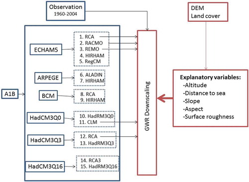
The flow chart of the general methodology using 15 different RCMs driven by six GCMs alongside the A1B carbon emission scenario and a geophysically based downscaling method is shown in Figure 2. The impact of the downscaling method on RCM-derived precipitation is carried out using only five RCMs from the 15 because of the high computation time that the GWR method requires. A performance test is, however, applied in selecting these five models. Daily and monthly time series for each RCM are generated with and without the downscaling method to use as a comparison for the reference and future scenario periods.

Figure 2. Flowchart of the methodology used.

3.1 GCM/RCM outputs

The climate model data used in this study are an ensemble of 15 RCMs from the ENSEMBLES project (van der Linden and Mitchell 2009). These 15 simulations are based on 11 RCMs (ALADIN, CLM, HadRM3Q0, HadRM3Q3, HadRM3Q16, HIRHAM, RACMO, RCA, RCA3, RegCM, REMO) driven by six different GCMs (ARPEGE, BCM, ECHAM5, HadCM3Q0, HadCM3Q3 and HadCM3Q16); their combinations are shown in Figure 2. Imperfections arising from model uncertainties and climate variability were well quantified in this project. The spatial resolution of all the models is 0.22° (approximately 25 km). With a nesting configuration, GCMs provide the initial and boundary conditions for RCMs. For all the models, daily and monthly precipitation time series are available for the time period 1951–2100. RCM climate data from the ENSEMBLES project are produced by considering the A1B carbon emission scenario, which predicts rapid economic growth and population increases until the middle of the 21st century, followed by the development of more efficient technologies and a population decrease. In this study, we consider the time periods of 1961–1990 and 2071–2100 as the reference and future (scenario) time periods, respectively. For the study area (sub-catchment 02-67 in Fig. 1), daily and monthly precipitation have been extracted from the 15 RCMs for the two periods, using the weighted-area interpolation of the nearest neighbouring grids occupying the catchment area.

3.2 GWR downscaling method

The GWR approach is a spatial statistics method used for analysing “spatial non-stationarity”, which is defined as being alterations in relationships between variables from one point (station) to another. GWR develops different equations for every station (point) in the datasets through the dependent and explanatory variables of the stations (ESRI 2014). Consequently, GWR provides valuable information about the nature of an investigated relationship and, in this way, it stands apart from other regression methods (Fotheringham et al. 2002), as it allows for the implementation of topographical and environmental conditions in the model. Furthermore, Bostan et al. (2012) pointed to the superiority of GWR for interpolating the annual precipitation in Turkey when compared to other conventional methods. GWR may be introduced as follows:

(1)

where is the dependent variable for observation i, is the intercept, is an estimated parameter of k, x_ik is the value of the kth variable for i, ε_i is the error term and are coordinates of i (Fotheringham et al. 2002). The concept here is that closer observations may affect one another’s parameters to a greater extent than observations that are further apart.

The GWR method has been used in several climate studies for estimating precipitation and temperature data. For example, using GWR, Kamarianakis et al. (2008) adjusted satellite-based precipitation estimates at the local scale in Mediterranean regions, while Wagner et al. (2012) estimated the spatial distribution of precipitation in local domains of monsoon climate regions, where climate stations are rare, using other interpolation techniques. Li et al. (2010) investigated the relationships between urban land surface temperature and explanatory variables. They claimed that the spatial non-stationary method, GWR, provided a better performance than other methods while allowing the implementation of topographical and environmental conditions in the model. The importance of the explanatory variables representing the spatiotemporal characteristics of geographical domains changes according to the prevailing climate and precipitation regimes of a particular region. To infer local geographical features in this study, the GWR downscaling method is used to produce monthly precipitation and temperature data at 1 km resolution from RCM climate data at 25 km resolution. The GWR method uses station precipitation or temperature data and some explanatory data (variables) for simulation. Explanatory variables representing the local characteristics of station points are altitude, aspect, slope, distance to sea and surface roughness. The aim of using explanatory variables is to reflect the impact of the topographical properties of stations in simulated results. Explanatory variables of RCM grids, meteorological stations and prediction points are determined using ASTER GDEM (30 m) data, a map of the study area formatted as a shape file, and classified LANDSAT 5 TM satellite images. Altitude, slope, aspect and the land cover values of meteorological stations are acquired from corresponding pixels after matching relevant maps with station points. The distances between station points and shorelines are calculated using an automatic function of ArcGIS. These variables are selected for this study because they functioned well for mapping the annual average precipitation of Turkey in Bostan et al. (2012).

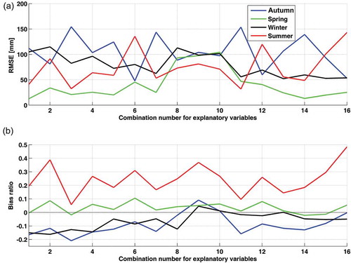
The GWR method is calibrated by using explanatory variables from eight meteorological stations located around the Omerli basin, in order to adjust the model for the local conditions of the study area. Sixteen different combinations among the explanatory variables are specified for calibrating the GWR along with the four seasons, and they are listed in Table 2. A sensitivity study for setting up the best combination of seasons among explanatory variables is performed. For each simulation, the GWR uses monthly precipitation data from dependent meteorological stations (seven of eight stations) and their explanatory variables, and makes a prediction at the independent station. This prediction is repeated eight times for each independent station that is not utilized in the GWR simulation. Seasonal total precipitation from monthly predictions and corresponding observations from free stations are compared to determine the best set of suitable variables for each season. Figure 3 shows the calculated mean root mean square error (RMSE) and bias ratio values for spring, summer, autumn and winter, along with 16 combinations. According to the lowest values of RMSE and the bias ratio in Figure 3, the best GWR models are selected as 1 for spring, 11 for summer, 16 for autumn, and 13 for winter. Sensitivity of explanatory variables to estimated precipitation changes with season, as the most suitable variables are implemented in the model with these selected combinations for each season. It is suggested that these selected combinations could be used in monthly predictions of the related seasons when downscaling the 25 km RCM grid to 1 km as a function of representative explanatory variables of RCM grids. While conducting downscaling, the variables and gridded monthly RCM precipitation represent predictors in these suggested combinations.

Table 2. Explanatory variables used in the GWR application (C: combination, VAR: variable).

	VAR. 1	VAR. 2	VAR. 3	VAR. 4	VAR. 5	WEIGHTS
C1	altitude	aspect	distance to sea	slope
C2	altitude	aspect	distance to sea	slope		altitude
C3	altitude	aspect	distance to sea	slope		aspect
C4	altitude	aspect	distance to sea	slope		slope
C5	altitude	aspect	distance to sea		surface roughness
C6	altitude	aspect	distance to sea		surface roughness	altitude
C7	altitude	aspect	distance to sea		surface roughness	aspect
C8	altitude	aspect		slope	surface roughness
C9	altitude	aspect		slope	surface roughness	altitude
C10	altitude	aspect		slope	surface roughness	aspect
C11	altitude		distance to sea	slope	surface roughness
C12	altitude		distance to sea	slope	surface roughness	altitude
C13	altitude		distance to sea	slope	surface roughness	slope
C14		aspect	distance to sea	slope	surface roughness
C15		aspect	distance to sea	slope	surface roughness	aspect
C16		aspect	distance to sea	slope	surface roughness	slope

Figure 3. (a) Mean RMSE and (b) bias ratio values calculated from GWR-simulated monthly precipitation at meteorological stations for 16 GWR combinations.

It is an important deficiency that spatial interpolation methods, such as kriging, spline and ordinary least square, are not able to make simulations in which the number of stations is small (Bayraktar et al. 2005). However, GWR is able to perform simulations among a small number of stations and RCM grids. The 16 RCM grids surrounding the Omerli basin are used to calculate their representative explanatory variables. The median value of the explanatory variables of these grids is determined by collocating the 30 m resolution variables within each 25 km RCM grid. Our initial assessment shows that the use of median values instead of means for explanatory variables in the model structure releases smaller errors in precipitation estimates. The metadata tool of ERDAS Imagine is used to calculate the median statistics for altitude, slope and aspect variables. After classifying the LANDSAT 5 TM satellite image using an unsupervised classification technique, the pre-defined values of roughness length determined for the USGS land cover types are applied to each land cover class. Finally, the land cover map is matched with grid borders and dominant land cover values determined for the grids. It is also necessary to determine the explanatory variables of the prediction points in order to run GWR. The variables for estimation grids are directly obtained from the re-sampled 1 km grid of the ASTER DEM data. Figure 4 shows the 16 RCM grids around the Omerli basin and 1 km prediction grids within the sub-catchment. The median values of explanatory variables for sixteen RCM grids are listed in Table 3.

Table 3. Calculated median values of explanatory variables for 16 RCM grids in the GWR application.

Grid	Altitude (m)	Aspect	Distance to sea (km)	Slope (%)	Surface roughness
1	110	21.54	7.6	4.42	50
2	268	51.15	10.48	7.43	50
3	89	10.27	9.27	6.37	50
4	80	361	6.39	5.9	50
5	68	361	5.67	4.72	50
6	111	361	7.96	5.67	50
7	288	7.46	9.31	9.78	50
8	527	44.1	11.24	11.46	50
9	0	361	3.91	0	0.1
10	258	73.67	11.63	8.97	50
11	97	32.82	4.3	7.09	50
12	30	361	4.68	3.22	0.1
13	0	361	0	0	0.1
14	0	361	0	0	0.1
15	0	361	0	0	0.1
16	0	361	0	0	0.1

Figure 4. The 16 numbered 25-km RCM grids around the Omerli basin and 1-km GWR prediction grids within the sub-catchment. The locations of meteorological stations are also shown.

3.3 Extreme precipitation index calculation

Extreme weather events are defined as “the occurrence of a value of a weather or climate variable above (or below) a threshold value near the upper (or lower) ends of the range of observed values of the variables” (IPCC 2012). Characteristics of precipitation extremes with respect to seasons, as well as all-year-round, are also evaluated to assess the changes in extreme precipitation in the catchment, using RCMs with and without the downscaling GWR method. Both model performance and future changes in extreme precipitation events are assessed by calculating the extreme precipitation index (EPI), as used by Sunyer et al. (2015).

The EPI is defined as the average change in extreme precipitation, which is higher than a defined return period. In this study, the return period is set equal to 1 or 5 years. EPI is estimated separately for each GWR, RCM, threshold return period, season and temporal aggregation for the Omerli sub-catchment. Four seasons are considered: winter (December to February), spring (March to May), summer (June to August) and autumn (September to November). Additionally, the index is estimated considering the entire time series, i.e. without dividing into seasons. The temporal aggregations considered are 1, 2, 5, 10 and 30 days. These are estimated using a moving average from the daily time series.

The first step in the calculation of EPI is to extract the extreme value series from the precipitation time series. The peak-over-threshold (POT) method is used for this purpose. Peaks are extracted using the 1- and 5-year threshold return levels. For example, with a 30-year record, the 30 and 6 most extreme events are included in the extreme series for the 1- and 5-year threshold levels, respectively. An independence criterion based on the inter-event time is applied to make sure that extreme values are independent, i.e. only values separated by more than Δt days are considered; Δt is set equal to the temporal aggregation, i.e. for an aggregation time of 1 day, events must be separated by more than 1 day. EPI is then estimated as:

(2)

where and are the averages of the selected POT values used as reference (observation) and scenario (referenced RCMs), respectively. EPI takes the value of 1 if no change is estimated from reference to scenario and is greater (less) than 1 if the average extreme precipitation is higher (lower) in the scenario time series.

4 Results

In the following sub-sections, evaluation results for RCM-derived precipitation with and without downscaling methods are presented by their general mean features on monthly and daily time scales, daily extreme precipitation indexes for different seasons, and extreme frequency distributions on daily and monthly time scales. These analyses are provided for both reference and future periods.

4.1 Mean precipitation analyses

General performance of RCMs and the downscaling technique is evaluated by capturing the mean properties of daily and monthly precipitation for the reference period (1961–1990). This assessment helps us to understand the reliability of future (2071–2100) projections obtained from each GCM/RCM system, together with the downscaling method. Figure 5 shows comparisons between the observed and simulated daily precipitation averaged over the reference period for each of the GCM/RCM combinations. Precipitation time series are shown with their 1-day and 30-day moving averages. The overall trend and important signals over the seasons are shown clearly alongside a 30-day search window, as it provides a smoother curve. Sub-plots identified with some models (1, 2, 3, 11, and 12) also show the corresponding precipitation time series according to GWR application. Prediction behaviour is variable for each model during the winter and spring, while all models except model 8 (BCM/RCA) underestimate precipitation during summer and autumn according to 1-day and 30-day moving averages. In particular, some models (1,2,3,4,6,7,9,12,14, and 15) show a strong dry bias in summer and autumn. The RCA (model 8) shows significant overestimation for spring and summer, but this feature is not available when it is initialized by different GCMs (ECHAM5 and HadCM3Q3) in models 1 and 12 over the same periods. The BCM model initialization may provide initial wet and boundary conditions for the RCA, which becomes sensitive to the convective scheme used in this RCM. On the other hand, for this particular study area, the same initialization from BCM for HIRHAM (model 9) does not release wet bias over the summer and spring periods. During the winter and spring periods, some models (1,2,4,6,10,11,13, and 15) overestimate the mean daily precipitation, while others either slightly underestimate or show a similar mean trend with observations. Among the 15 models, only two (14 and 4) show the underestimation feature throughout the year for the study area. When the downscaling is applied to RCM grids from models 1, 2, 3, 11 and 12, there is substantial improvement in daily mean precipitation represented by 1-day and 30-day moving averages. The seasonal observed trends for autumn, winter and spring are followed better with GWR application for each of these models (see relevant subplots in Fig. 5). The daily simulated precipitations with and without the GWR averaged over five RCMs for a 30-day moving window are compared with observed precipitation (see Fig. 6). The mean of these five RCMs without downscaling indicates underestimation throughout the year; this becomes significant during summer, autumn and winter. The GWR not only reduces the error in mean precipitation but also improves the general seasonal trend by capturing important signals in daily observed precipitation. However, the increased quantity in mean precipitation with GWR does not preclude underestimation during summer and autumn, while causing overestimation from February to May.

Figure 5. Comparisons between observed and simulated daily precipitation averaged over the reference period for each of the GCM/RCM combinations. Precipitation time series are shown with their 1-day and 30-day moving averages. Each figure panel belongs to an individual model. Subplots identified with some models (1, 2, 3, 11 and 12) also show the corresponding precipitation time series according to GWR application.

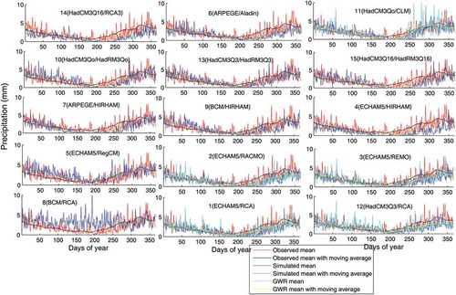
Figure 6. Daily simulated precipitation, with and without GWR, averaged over five RCMs for a 30-day moving window compared with observed precipitation.

The mean RMSE, bias, bias ratio and standard deviation of each model combination are calculated for a 30-day moving-average data series along with the reference period and are shown in Table 4. The performance of the models in representing the mean behavioural trend of daily precipitation is measured using different model set-ups, in which the same RCMs are coupled with different GCMs and vice versa. Two of the models (5 and 8) show a wet mean bias (positive bias) throughout the entire reference period in this study area. The HIRHAM coupled with BCM, instead of ARPEGE and ECHAM5, gives the lowest biased values (−0.13 and −0.06 for bias and bias ratio) and error (0.75). Similarly, the RCA initialized with ECHAM5 provides the lowest biases (−0.48 mm and −0.22 mm for bias and bias ratio) and error (0.66 mm) when compared to initializations from BCM and HadCM3Q3. Overall, model 13 released the best statistical measures (−0.09, −0.04 and 0.54 mm for bias, bias ratio and RMSE, respectively) among the 15 model pairs for this particular study area. The GWR downscaling method greatly improved the mean properties of daily precipitation by releasing reduced mean bias and error for five models (1, 2, 3, 11, 12). The standard deviations of each model pair for daily precipitation estimates highlight the partitioning of variability (uncertainty) between GCMs and RCMs. Greater variability (higher deviations from mean during the period) is obtained from RCMs coupled with the same GCMs than those from GCMs linked with the same RCMs. For example, the mean standard deviation from RCM variability is 1.002 mm, while it is 0.879 mm from GCM variability.

Table 4. Mean RMSE, bias, bias ratio and standard deviation (SD) of each model pair calculated from a 30-day moving-average data series and the reference period. Underlined bold characters represent values from the HIRHAM RCM initialized by ECHAM5, ARPEGE and BCM (4, 7, 9); italic bold characters represent statistics for the RCA model initialized by ECHAM5, BCM and HadCM3Q3 (1, 8, 12). Other models (1–5, 6–7, 8–9, 10–11, 12–13, 14–15) provide values from different regional climate models initiated by the same GCM. The values in parentheses are from the GWR method applied to the specific RCM model.

GCM/RCM		SD	Bias	Bias ratio	RMSE
1	0.8785		−0.4884 (−0.2150)	−0.2242 (−0.0987)	0.6663 (0.5167)
2	0.8965		−0.7132 (−0.5435)	−0.3275 (−0.2495)	0.8446 (0.7186)
3	0.9230		−0.6281 (−0.3657)	−0.2884 (−0.1679)	0.7178 (0.5597)
4	0.8385		−1.0667	−0.4898	1.1987
5	1.0188		0.5019	0.2305	0.7479
6	0.8803		−0.4788	−0.2198	0.8968
7	1.2504		−0.6725	−0.3088	0.8263
8	0.3806		1.0444	0.4790	1.5059
9	1.2094		−0.1313	−0.0603	0.7533
10	1.3190		−0.0537	−0.0247	0.7759
11	1.2713		−0.2059 (−0.1059)	−0.0946 (−0.0486)	0.5166 (0.4682)
12	0.7203		−0.4928 (−0.1856)	−0.2263 (−0.0852)	0.8369 (0.7191)
13	1.1965		−0.0937	−0.0430	0.5402
14	0.8113		−0.9483	−0.4354	1.1114
15	1.1694		−0.4266	−0.1958	0.8322

Figure 7 shows comparisons between observed and simulated monthly mean precipitation averaged from five models (1, 2, 3, 11, 12) over the reference period for models without downscaling (a) and with downscaling (b). Standard deviations for five models for monthly mean precipitation are also indicated in these plots. Monthly simulated values are well matched with observations from February to June, although a discrepancy between observed and estimated values exists in other months prior to and following application of the GWR method to RCM grids. A small but nonetheless important removal of this discrepancy occurs in winter, autumn and spring months with GWR application. During spring months (March, April, May and June), the error bars of downscaled precipitation are substantially smaller than those of the original RCMs, indicating similar performance among all RCMs in capturing the observed spring precipitation. From February to May, models slightly overestimate monthly precipitation, while they underestimate it from June to January. The GWR tends to modify this feature in the models in spring, autumn and winter months, throughout which downscaling reduces the errors.

Figure 7. Monthly mean precipitation of five RCMs compared with observed precipitation averaged (a) over the reference period for original RCMs, and (b) for downscaled RCM precipitation. Standard deviations for five models for monthly mean precipitation are also indicated.

4.2 Extreme precipitation evaluation

The EPI value is calculated between observation and original RCMs and observation and downscaled RCMs for the reference period. With these analyses, we measure the error of the GWR method in downscaling the RCM outputs for extreme precipitation and evaluate the performance of the RCMs in representing extreme precipitation. In this way, they allow us to assess whether the error in the downscaled time series is smaller than in the RCMs.

The box plots for extreme precipitation indexes from five RCMs (1, 2, 3, 11, 12) for five different moving windows (1, 2, 5, 10 and 30 days) during the four seasons (DJF for winter, MAM for spring, JJA for summer and SON for autumn), and all year are shown in Figure 8(a) and (b) for 1-year and 5-year return levels, respectively, while the equivalent plots for downscaled precipitation from the same RCM grids are shown in Figure 8(c) and (d). In all seasons, the models underestimate extreme precipitation, as EPI values are below 1 for both return levels (see Fig. 8(a) and (b)). The highest errors in extreme precipitation occur in spring and autumn, while the lowest errors occur in winter and summer. As the aggregation time (search window for moving average) increases from 1 day to 30 days, the error decreases or the median of EPI approaches 1 for all seasons and all year. With the application of the GWR method, errors in extreme precipitation are greatly reduced for all seasons for both return levels (see Fig. 8(c) and (d)). The underestimation feature of models is significantly modified for all moving windows. The boxes and their medians move towards an EPI value of 1 after using the GWR method. For example, all median values of boxes in winter show an EPI greater than 1 and this yields overestimation for winter extreme precipitation. The highest variability in extreme precipitation among models occurs in winter, and it appears that GWR has no influence on this property.

Figure 8. Box plots of extreme precipitation indexes from five RCMs for five different search windows for winter (DJF), spring (MAM), summer (JJA) and autumn (SON), as well as all year, for (a) a 1-year return level, and (b) a 5-year return level; and equivalent plots using a GWR method for (c) a 1-year level, and (d) for a 5-year level. Search windows from left to right are for 1, 2, 5, 10 and 30 days. On each box, the central mark represents the median; the lower and upper edges of the box are the 25th and 75th percentiles, respectively. The whiskers extend to the most extreme data points that are not considered outliers; outliers are shown as plus signs. The whisker length is 1.5 (default value).

4.3 Changes in extreme precipitation

The EPI is used to compare changes in the original and downscaled time series from reference to future periods. This allows us to compare the changes estimated from the downscaled precipitation through GWR to the changes projected by the RCMs.

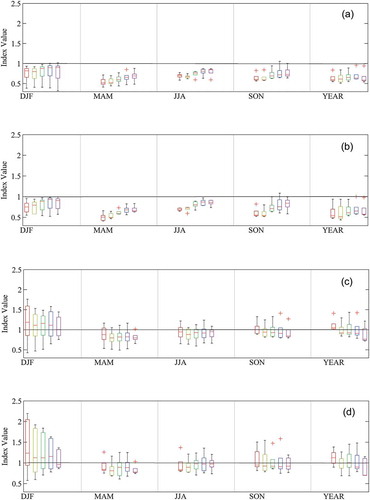
The box plots of EPI from five RCMs for five different aggregation periods (1, 2, 5, 10 and 30 days), along with the four seasons and all year are shown in Figure 9(a) and (b) for 1-year and 5-year return levels, respectively. In general, winter, spring and summer periods show an increase in extreme precipitation in all search windows, as the medians of EPI for five RCMs are greater than 1 during these seasons. The highest increase in extreme precipitation is obtained within the summer period, particularly for 10- and 30-day search windows. For example, the median value is greater than 1.5 for summer, while in winter and spring, median index values are around 1.1. Extreme precipitation decreases for 1-, 2-, and 30-day search windows in autumn; however, other search windows in this season also show an increase in extreme precipitation. Therefore, the change in extreme precipitation is not consistent across search windows in autumn. When evaluating the yearly index values, the change in extreme precipitation from reference to future periods is insignificant for 5-, 10- and 30-day search windows, as their median index is nearly 1, with very small box sizes. However, the 1- and 2-day search windows indicate an important decrease in extreme precipitation, which is mostly caused by the high number of rainy days used in the reference period in autumn. In all seasons with a 5-year level, larger changes and variability are obtained, as extreme precipitation events become more significant.

Figure 9. Index values of extreme precipitations from five RCMs for five different search windows for winter (DJF), spring (MAM), summer (JJA) and autumn (SON), as well as all year, for (a) a 1-year level, and (b) a 5-year level; and equivalent plots using a GWR method for (c) a 1-year level, and (d) a 5-year level. Search windows from left to right are for 1, 2, 3, 10 and 30 days.

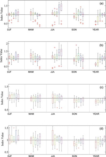
Comparing the changes obtained from the GWR method with the mean changes projected by the RCMs (see Fig. 9(c) and (d)), there are generally significant modifications (up to 35% for summer with 10- and 30-day search windows) to the changes estimated from the uncorrected RCM projections. With a 1-year level, the median EPI of each box for all search windows is greater than 1 for winter, spring and summer, while it is below 1 for autumn and all year. These changes in the median values become more significant for spring, summer, autumn and yearly analyses at 5-year level. It appears that consistency in the modification to the changes degrades among search windows in winter at 5-year level. Nonetheless, the seasonal extreme precipitation increases in winter, spring and summer, and decreases in autumn from the reference to the future period. These changes are significantly modified and become more consistent across search windows when they are compared with the uncorrected RCMs (see Fig. 9(a) and (b)). The Omerli basin indicates an increase in precipitation extremes during winter, spring and summer, and a decrease during autumn and yearly analyses by the end of this century. This feature becomes more consolidated with downscaled values. It should be noted that downscaling methods that do not explicitly correct or take into account changes in extreme precipitation may lead to climate change signals different from those projected by the RCMs and should not be used.

4.4 Frequency analysis

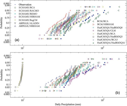
The influence of the GWR used with respect to the difference between the change projected by the uncorrected RCMs and the downscaled data is analysed by conducting frequency analyses using a data series of maximum daily peak and maximum monthly peak precipitations. According to our analyses, the log-normal function is a good fit to the maximum precipitation data and, therefore, we decided to use this distribution function in the frequency analyses. Figure 10 shows the probability of non-exceedence vs daily precipitation values from observation and 15 RCMs in (a) and (b) for the reference and future periods, respectively. With higher daily precipitation, the performance of all RCMs when following the observed frequency curve worsens. Among 15 RCMs, only BCM/RCA (8) indicates an overestimation in the frequency distribution. There is great variability among models in estimating the probability of non-exceedence, and this is more apparent towards higher precipitation amounts. The ECHAM5/RCA (1) model follows the observed frequency curve better than other models. In the future period, the curves follow a more compact feature than models comparing the reference period. In addition, most of the models (12 altogether) produce higher (lower) precipitation amounts (return period) for a given exceedence probability (precipitation amount) in the future period. This situation is evident once the modelled frequency curves are compared with an observed frequency that is a baseline and remains unchanged in the future period. Three models, HadCM3Q3/HadRM3Q3 (13), HadCM3Q3/RCA (12) and BCM/RCA (8) show the opposite behaviour (decreased precipitation amount for a given probability) in the frequency curves for the future period.

Figure 10. Probability of non-exceedence vs daily precipitation for observations and 15 RCMs for (a) the reference period, and (b) the future period. The observed frequency curve (bold, blue dots) is given in the future period as a baseline.

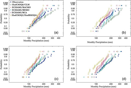
Figure 11 shows a comparison between observed and RCM-derived frequency curves of maximum monthly precipitation with the use of downscaling in (a) and (b) for the reference and future periods, respectively, while the equivalent plots from the original five RCMs (without downscaling) are provided in (c) and (d). Skill in following the observed frequency curve using models is improved for all exceedence probability ranges using the downscaling method (see Fig. 11(a)–(c)). The underestimation behaviour of the original RCMs towards higher precipitation amounts is modified using the downscaling method and thus the magnitude of extreme monthly precipitation is increased for a given exceedence probability (or return period). For example, the HadCM3Qo/CLM (11) overestimates precipitation for all ranges of probability values using downscaling. In regard to the downscaling method, the ECHAM5/REMO (3) yields the best performance in following the observed frequency curve for monthly precipitation. In the future period, except for the HadCM3Q3/RCA (12), all models provide higher monthly precipitation amounts for a given exceedence probability than those in the reference period (see Fig. 11(c)–(d)). This feature is more pronounced when the downscaling method is applied to RCM grids (Fig. 11(a)–(b)). The GWR method evaluated using five RCMs preserves the original climate change signal produced by each RCM. For example, model 12 is modified towards its original trend, which shows a decrease in precipitation magnitude from the reference to the future period.

Figure 11. Probability of non-exceedence vs maximum monthly precipitation for observations and five downscaled RCMs for (a) the reference period and (b) the future period, with equivalent plots from the original five RCMs for (c) the reference period and (d) the future period. The observed frequency curve (bold, blue dots) is given in the future period as a baseline.

5 Summary discussion and conclusions

In this study, a climate change impact assessment concerning precipitation in the Omerli basin of Istanbul, Turkey, is carried out by observing the changes in mean and extreme precipitation throughout the four seasons and annually for reference (1960–1990) and future (2070–2100) periods. Simulations from 15 different GCM/RCM scenarios in the EU-ENSEMBLES project are used in this study, as the ensemble approach improves forecast accuracy and decreases uncertainties. The grid scale obtained from RCMs is relatively coarse when compared to the conceptual small watershed scale and remains poor at representing extreme precipitation. Therefore, a finer resolution downscaling technique is necessary prior to practical hydro-meteorological applications. A geo-statistical downscaling method relying on the local geophysical (explanatory) parameters of grids or stations is developed to downscale RCM precipitation from 25 km to 1 km.

Comparisons are made between modelled and observed daily precipitation data from climate stations with and without the downscaling method to investigate the improvement (or otherwise) in the ability of RCMs to describe the mean, extreme and frequency values of surface precipitation during the reference period. Extreme index values, described as the ratio between the mean extreme series for the reference period and mean extreme series for the scenario period, are calculated for each season to determine the changes from the past to the future for the magnitudes of precipitation under the influence of a downscaling technique. Frequency behaviour of simulated extreme daily precipitation is shown to assess whether the extreme magnitude increases or decreases under the influence of downscaling for a given return period during the future period.

For all seasons, the RCM-GCM projections are the main source of variability in the precipitation results; additionally, the RCMs represent a larger percentage of the total variability than the GCMs, especially in summer. This is attributable to the sensitivity of different convective schemes used in each RCM, because precipitation extremes occur mostly from local convections during the summer in the Omerli basin. For example, the HadCM3Qo/CLM (11) provided the best results for the frequency distributions of precipitation among the 15 RCMs in this study area. However, this model may not provide the same accuracy for other study regions, depending on the geographical conditions and climate system that affect the performance of the physics used in these models. Therefore, as stated in the literature (e.g. Sunyer et al. 2015), the multi-model ensemble method (instead of a single model) is recommended for use in climate change impact studies. The results demonstrate that climate projections show large variations in the magnitude of the projected climate change signals. In some cases, the simulated changes even point in different directions (8, 12, and 13). As addressed in other studies, the downscaling method is an important tool for reducing the uncertainty related to climate model projections. This study also contributes to this issue by focusing on the representation of extreme precipitation events through the application of a geo-statistical downscaling technique, which is different from the statistically based methods commonly used in the literature.

By improving the representation of extreme precipitation from the RCMs, the GWR method is able to preserve the climate change signal originated by GCM/RCM coupling. It should be noted that downscaling methods that do not explicitly correct or take into account changes in extreme precipitation may lead to different climate change signals than the ones projected by the RCMs and should not be used. This study illustrates that there is a large variability in the changes estimated from GWR and RCMs. The selection of a suitable GWR model depends on the physical geographical characteristics of the catchment throughout four different seasons. The projected seasonal changes (increases in winter, spring and summer and decrease in autumn) in extreme precipitation should be considered in planning regarding the Omerli Dam reservoir in order to sustain effective storage and use of water. The frequency distribution analyses suggest that the Omerli basin and its adjacent water supply areas in Istanbul Province will experience extreme precipitation events with much shorter recurrence times in the future. For designing and operating water-related structures, the intensity–duration–frequency (IDF) curves should be adapted to current and future climate conditions. These results should be used in the Omerli Dam’s future water management policies and can potentially provide support for research and decision making in the science and policy making arenas. As stated by Beven (2011), we need better precautionary approaches for planning future consequences related to climate change (and the potential impacts of other catchment changes). Also, Kundzewicz and Stakhiv (2010) suggested that we should indeed improve climate models so that they are more useful for the next level of analysis, beyond broad policy-type statements on mitigation strategies such as adaptation strategies – especially as applied to the design of hydraulic structures.

The primary conclusions that can be drawn from the research described in this study are as follows:

• RCMs show greater variability than GCMs in projected mean precipitation. Downscaling has a strong influence on mean precipitation and, in particular, on extremes.

• All RCMs with varying magnitude show an underestimation tendency in mean precipitation during summer, autumn and early winter and most overestimate the mean precipitation during late winter and spring. All models underestimate mean extreme precipitation during all seasons.

• The lowest errors in predicting extreme precipitation are obtained for winter and the highest errors are obtained for spring. GWR improves the underestimation tendency of RCMs; this improvement is found to be significantly better in the representation of extreme values.

• Changes in extreme precipitation from the reference to the future period are significantly modified (up to 35%) by the presence of downscaling. The autumn season has a strong effect on annual extreme precipitation, as it is attributable to a decrease in annual precipitation. The changes obtained for different temporal aggregations also depend on the physical geographical characteristics of the catchment and season analysed, i.e. there is no general tendency for an increase or decrease in the extreme precipitation index with increasing temporal aggregation.

• All RCMs without GWR underestimate the observed daily precipitation frequency, but this feature is significantly improved with the application of downscaling.

• The majority of RCMs, regardless of the downscaling method, show that the magnitudes of extremes for given return periods increase in the future. Again, this behaviour is more distinctive with GWR. Modified changes with GWR preserve the climate change signal produced by RCMs.

Acknowledgements

We thank to two anonymous reviewers and associate editor Dr. James Ward for their valuable comments in improving the content of the paper.

Disclosure statement

No potential conflict of interest was reported by the authors.

Additional information

Funding

This study is supported by European procedures for flood frequency estimation (FloodFreq) Cost Action (ES0901) and the TÜBİTAK ARDEB ÇAYDAG Scientific and Technological Research Project Programme (1001) with Project no. 110Y036.

References

- Anagnostopoulos, G.G., et al., 2010. A comparison of local and aggregated climate model outputs with observed data. Hydrological Sciences Journal, 55 (7), 1094–1110. doi:10.1080/02626667.2010.513518
- Bayraktar, H., Turalioglu, F.S., and Şen, Z., 2005. The estimation of average areal rainfall by percentage weighting polygon method in Southeastern Anatolia Region, Turkey. Atmospheric Research, 73, 149–160. doi:10.1016/j.atmosres.2004.08.003
- Beniston, M., et al., 2007. Future extreme events in European climate: an exploration of regional climate model projections. Climate Change, 81, 71–95. doi:10.1007/s10584-006-9226-z
- Beven, K., 2011. I believe in climate change but how precautionary do we need to be in planning for the future? Hydrological Processes, 25, 1517–1520. doi:10.1002/hyp.v25.9
- Birsana, M.-V., et al., 2005. Streamflow trends in Switzerland. Journal of Hydrology, 314, 312–329. doi:10.1016/j.jhydrol.2005.06.008
- Bostan, P., Heuvelink, G.B.M., and Akyurek, Z., 2012. Comparison of regression and kriging techniques for mapping the average annual precipitation of Turkey. International Journal of Applied Earth Observation and Geoinformation, 19, 115–126. doi:10.1016/j.jag.2012.04.010
- Brundson, C., Fotheringham, A., and Charlton, M., 1996, Geographically weighted regression: a method for exploring spatial nonstationarity. Geographical Analysis, 28, 281–298.
- Christensen, J.H., et al., 2007. Climate Change 2007: The Physical Science Basis—Contribution of Working Group I to the Fourth Assessment Report of the Intergovernmental Panel on Climate Change. Cambridge, UK: Cambridge University Press.
- Christensen, J.H. and Christensen, O.B., 2003. Climate modelling: severe summertime flooding in Europe. Nature, 421, 805–806. doi:10.1038/421805a
- Derin, Y. and Yilmaz, K.K., 2014. Evaluation of multiple satellite-based precipitation products over complex topography. Journal of Hydrometeorology, 15 (4), 1498–1516. doi:10.1175/JHM-D-13-0191.1
- Döll, P., et al., 2015. Integrating risks of climate change into water management. Hydrological Sciences Journal, 60 (1), 4–13. doi:10.1080/02626667.2014.967250
- ESRI (Environmental Systems Research Institute), 2014. ArcGIS Help 10.1. ArcGIS Resources. Available from: http://resources.arcgis.com/en/help/main/10.1/index.html#/What_are_geostatistical_interpolation_techniques/003100000031000000/ [ Accessed 24 Jun 2014].
- Ezber, Y., et al., 2006. Climate effects of urbanization in Istanbul: a statistical and modeling analysis. International Journal of Climatology, 26, 1225–1236.
- Field, C.B., et al., eds., 2012. Managing the risks of extreme events and disasters to advance climate change adaptation. Special report of working groups I and II of the Intergovernmental Panel on Climate Change (IPCC). Cambridge: Cambridge University Press [online]. Available from: http://www.ipcc.ch/pdf/special-reports/srex/SREX_Full_Report.pdf [Accessed 23 Oct 2014].
- Fotheringham, A.S., Brunsdon, C., and Charlton, M.E., 2002. Geographically weighted regression: the analysis of spatially varying relationships. Chichester: Wiley.
- Fowler, H.J., Blenkinsop, S., and Tebaldi, C., 2007. Linking climate change modelling to impacts studies: recent advances in downscaling techniques for hydrological modelling. International Journal of Climatology, 27, 1547–1578. doi:10.1002/joc
- Gleckler, P.J., Taylor, K.E., and Doutriaux, C., 2008. Performance metrics for climate models. Journal of Geophysical Research: Atmospheres, 113, D06104.
- IBB (Istanbul Metropolitan Municipality), 2014. İstanbul İl ve İlçe Alan Bilgileri, June 15. Available from: http://www.ibb.gov.tr/tr-tr/kurumsal/pages/ilceveilkkademe.aspx [ Accessed 8 Sep 2014].
- IPCC, 2007. Climate Change 2007: the physical science basis, summary for policymakers. Contribution of Working Group I to the Fourth Assessment Report of the IPCC.
- IPCC, 2012. Glossary of terms. In: C.B. Field, et al., eds. Managing the risks of extreme events and disasters to advance climate change adaptation. A Special Report of Working Groups I and II of the Intergovernmental Panel on Climate Change (IPCC). Cambridge, UK: Cambridge University Press, 555–564.
- IWSA (Istanbul Water and Sewerage Administration), 2009. Geçmişten günümüze İstanbul’da suyun yönetimi. Rapor, İstanbul: İSKİ.
- Kamarianakis, Y., et al., 2008. Evaluating remotely sensed rainfall estimates using nonlinear mixed models and geographically weighted regression. Environmental Modelling & Software, 23, 1438–1447. doi:10.1016/j.envsoft.2008.04.007
- Kara, F. and Yucel, I., 2015. Climate change effects on extreme flows of water supply area in Istanbul: utility of regional climate models and downscaling method. Environmental Monitoring and Assessment, 187. doi:10.1007/s10661-015-4808-8
- Kjellström, E., et al., 2005. A 140-year simulation of European climate with the new version of the Rossby Centre regional atmospheric climate model (RCA3). Reports Meteorology and Climatology, Vol. 108. Sweden: SMHI, 54 pp.
- Knutti, R., et al., 2010. Challenges in combining projections from multiple climate models. Journal of Climate, 23, 2739–2758. doi:10.1175/2009JCLI3361.1
- Koutsoyiannis, D., et al., 2011. Scientific dialogue on climate: is it giving black eyes or opening closed eyes? Reply to “A black eye for the Hydrological Sciences Journal” by D. Huard. Hydrological Sciences Journal, 56 (7), 1334–1339. doi:10.1080/02626667.2011.610759
- Kundzewicz, Z.W. and Stakhiv, E.Z., 2010. Are climate models “ready for prime time” in water resources management applications, or is more research needed? Hydrological Sciences Journal, 55 (7), 1085–1089. doi:10.1080/02626667.2010.513211
- Li, S., et al., 2010. Investigating spatial non-stationary and scale-dependent relationships between urban surface temperature and environmental factors using geographically weighted regression. Environmental Modelling & Software, 25, 1789–1800. doi:10.1016/j.envsoft.2010.06.011
- Morán-Tejeda, E., et al., 2011, River regimes and recent hydrological changes in the Duero Basin (Spain). Journal of Hydrology, 404 (3–4), 241–258. doi:10.1016/j.jhydrol.2011.04.034
- Schmocker-Fackel, P. and Naef, F., 2010. More frequent flooding? Changes in flood frequency in Switzerland since 1850. Journal of Hydrology, 381, 1–8. doi:10.1016/j.jhydrol.2009.09.022
- Stakhiv, E.Z., 2010. Practical approaches to water management under climate change uncertainty. In: H.H.G. Savinje, S. Demuth, and P. Hubert, eds. Hydrocomplexity: new tools for solving wicked water problems. Wallingford: IAHS Press, IAHS Publ, 338 pp.
- Sunyer, M.A., et al., 2015. Inter-comparison of statistical downscaling methods for projection of extreme precipitation in Europe. Hydrology and Earth System Sciences, 19, 1827–1847. doi:10.5194/hess-19-1827-2015
- Tebaldi, C. and Knutti, R., 2007. The use of the multi-model ensemble in probabilistic climate projections. Philosophical Transactions of the Royal Society A: Mathematical, Physical and Engineering Sciences, 365, 2053–2075. doi:10.1098/rsta.2007.2076
- van der Linden, P. and Mitchell, J., 2009. ENSEMBLES: climate change and its impacts: summary of research and results from the ENSEMBLES project. Exeter: Met Office Hadley Centre.
- Wagner, P.D., et al., 2012. Comparison and evaluation of spatial interpolation schemes for daily rainfall in data scarce regions. Journal of Hydrology, 464–465, 388–400. doi:10.1016/j.jhydrol.2012.07.026
- Wilby, R.L., 2010. Evaluating climate model outputs for hydrological applications. Hydrological Sciences Journal, 55 (7), 1090–1093. doi:10.1080/02626667.2010.513212
- Wilby, R.L., et al., 2004. Guidelines for use of climate scenarios developed from statistical downscaling methods, technical report, Intergovt. Panel on Clim. Change, Geneva, Switzerland.
- Yilmaz, K.K. and Yazicigil, H., 2011. Potential impacts of climate change on Turkish Water Resources: a review. In: A. Baba, et al., eds. Issues of national and global security series: NATO science for peace and security series C: environmental security, Vol. 3, 1st ed. Dordrecht, The Netherlands: Springer, 318 pp.
- Yucel, I., Güventürk, A., and Sen, O.L., 2015. Climate change impacts on snowmelt runoff for mountainous transboundary basins in eastern Turkey. International Journal of Climatology, 35, 215–228. doi:10.1002/joc.2015.35.issue-2