An approach for the determination of precipitation input for worst-case flood modelling

ABSTRACT

There is a lack of suitable methods for creating precipitation scenarios that can be used to realistically estimate peak discharges with very low probabilities. On the one hand, existing methods are methodically questionable when it comes to physical system boundaries. On the other hand, the spatio-temporal representativeness of precipitation patterns as system input is limited. In response, this paper proposes a method of deriving spatio-temporal precipitation patterns and presents a step towards making methodically correct estimations of infrequent floods by using a worst-case approach. A Monte Carlo approach allows for the generation of a wide range of different spatio-temporal distributions of an extreme precipitation event that can be tested with a rainfall–runoff model that generates a hydrograph for each of these distributions. Out of these numerous hydrographs and their corresponding peak discharges, the physically plausible spatio-temporal distributions that lead to the highest peak discharges are identified and can eventually be used for further investigations.

Editor A. Castellarin; Associate editor E. Volpi

KEYWORDS:

• Extreme floods
• precipitation distribution
• worst-case
• Monte Carlo

1 Introduction

Planning highly sensitive buildings and infrastructure (e.g. nuclear power plants, dams) often requires flood return level predictions that exceed the scope of today’s methods. Indeed, extreme floods with return periods up to 10 000 years have to be estimated in some cases. Proper methodical procedures, however, are still missing; estimating such extreme flood peaks in a probabilistic, stochastic or combined way based on relatively short time series (<100 years) of discharge and precipitation data, or both, is not expedient. These approaches can be applied to estimate events with return periods only two to three times longer than the measured periods (Institute of Hydrology 1999, Coles 2004).

There are two different conceptual approaches that can be leveraged to estimate very low probability floods: a statistical approach based on observed data and a physical approach based on calculated maximum precipitation. The first approach relates peak discharges to return levels and is based on observed input data, which are used to feed rainfall–runoff models. However, with regard to predicting floods with very low probabilities, the methodical challenge of this approach lies in determining precipitation input, as scenarios with very low probabilities are required. To achieve a wider variety of precipitation events, the input dataset can be expanded in different ways. Several studies have produced a wide range of possible precipitation scenarios by resampling techniques (Brandsma and Buishand 1998, Paquet et al. 2013), precipitation generators (Leander et al. 2005, Furrer and Katz 2008, Semenov 2008, Vandenberghe et al. 2010), statistical description of storm structures (Salvadori and De Michele 2006, Langousis et al. 2013) and bootstrap techniques (Uboldi et al. 2014). Such approaches can considerably improve the representation of spatio-temporal precipitation variability. However, they are still dependent upon manually pre-defined distribution functions and measured precipitation events. As can be concluded based on Verhoest et al. (2010), these methods aim mainly to reproduce rainfall time series in time and space. Moreover, Rogger et al. (2012a) show that the results of design flood estimations conducted in this way depend strongly on the applied method and furthermore on how the chosen method is applied. Even with specific modifications to the method (e.g. the use of information from historical floods), extreme value statistics does not allow for a reliable prediction of floods with return levels of 1000 years or more (e.g. Schumann 2007, 2012, Merz and Blöschl 2008).

As the methodical difficulties of predicting design floods with return levels of 1000 years or more are possibly insurmountable, it is appropriate to replace the prediction of events with very high return levels with a concept based on very unlikely events. This calls for the second approach, which examines the physical system boundaries in order to set an upper limit for a possible worst case flood, but does not relate an estimation of a worst-case peak discharge with a probability and hence a return period. In this case, calculated probable maximum precipitation (PMP) amount is distributed over the catchment in space and time to feed a rainfall-runoff model and calculate a possible worst-case flood. The PMP is defined as “the theoretical maximum precipitation for a given duration under modern meteorological conditions” (WMO 2009). The PMP is used to estimate a probable maximum flood (PMF), which is defined as “the theoretical maximum flood that poses extremely serious threats to the flood control of a given project in a design watershed” (WMO 2009). Although this technique is widely used in daily practice, it is limited by two factors. Firstly, the concept of PMP implies the existence of a physical upper limit for areal precipitation, which does not necessarily exist (Koutsoyiannis 1999, Papalexiou and Koutsoyiannis 2006, Papalexiou et al. 2013). Secondly, the concept of PMP/PMF has been more or less “static”, neglecting to sufficiently account for the decisive impact of temporal and spatial precipitation distribution on flood magnitude, i.e. only a few distributions have been considered so far.

Various approaches for the distribution of the PMP in space and time have been established, e.g. the station-average method, the Thiessen polygon method and the isohyetal method (McCuen 2005, Beauchamp et al. 2013). These methods aim to distribute the PMP in accordance with spatial and temporal patterns of observed data. The disadvantage of these methods is that they lack the flexibility needed to produce a wide variety of distribution scenarios. Over the last two decades, the complexity of PMP distribution approaches has risen along with the increase in computation power. Approaches such as the stochastic storm transposition approach by Foufoula-Georgiou (1989) and Franchini et al. (1996) and the phase-state approach by Dodov and Foufoula-Georgiou (2005) have been established. These approaches aim to probabilistically reproduce patterns and parameters of observed storms. The main assumption underlying these approaches is that an appropriate storm regionalization is reasonable despite orographic and climatic influences. According to the authors, the approaches are able to produce realistic spatio-temporal precipitation distributions with very low occurrence probabilities. However, the produced storms and their parameters are still dependent on observed events and the estimation of the “tail-behaviour” of distribution functions, and therefore they may exclude improbable but physically possible distributions.

Thus, there is still a need for methods that adequately deduce precipitation scenarios with very low probabilities. The present study complements the physical system boundary approach for flood prediction with a new procedure to generate appropriate input data. The approach is based on the physical limits of precipitation and should contribute to a more reliable estimation of very unlikely events. In contrast to the existing precipitation distribution approaches, which are either relatively inflexible (station-average, Thiessen polygon, isohyetal distribution) or dependent on observations (stochastic storm transposition, phase-state), the proposed approach provides a method for generating a high number of spatio-temporal distributions of extreme precipitation and then identifying the potentially most hazardous distributions. The results can first be used to force sophisticated hydrological and hydraulic models, where the runoff processes during extreme events and specific side effects (e.g. landslides, inundations or log jams) can be taken into consideration for PMF estimation. Secondly they can be applied to rapidly estimate the likely distribution of peak discharges induced by a given amount of precipitation.

2 Method

The basic concept of the proposed approach entails testing numerous spatio-temporal distributions of extreme precipitation in a given catchment. Any one of the generated spatio-temporal distributions is used to iteratively force a simple model, as presented in the model design section. How these spatio-temporal distributions are generated is examined in the areal precipitation section. Finally, as explained in the model output section, the model generates one hydrograph for each generated spatio-temporal precipitation distribution. The spatio-temporal distributions leading to the highest peak discharges according to the model can then be used for further analyses.

2.1 Hydrological model

The transition from rainfall to runoff is calculated by a hydrological model. In this case, it is appropriate to choose a relatively simple model and to keep the computation time low. The model used in this study can be built for any desired mesoscale catchment, customized for the catchment-specific conditions. Firstly, the catchment is divided into meteorological regions, taking into account the geographical and meteorological patterns within the basin. The meteorological regions will later be used to achieve a physically plausible precipitation distribution (as explained in Section 2.2). The relevant catchments within the meteorological regions are identified in order to depict distribution on a finer scale. The main criterion for this division is the availability of gauging stations. A schematic example of a possible model design is shown in Figure 1.

Figure 1. Sample scheme for a possible model set-up. The model is embedded in a Monte Carlo framework to detect worst-case spatio-temporal precipitation distributions.

Runoff is modelled with a combination of unit hydrographs as proposed by Dooge (1959) and a simple routing for taking the flow durations between the catchments into account. Lakes inside a basin are handled as single linear storages; the outflow of the lakes can be estimated with rating curves describing the relationship between water level and discharge.

Plausible runoff coefficients are required to apply the described model. Based on former studies and considering the basin-specific characteristics, assumptions have to be made to estimate runoff coefficients in a practical way. In line with the aim of the proposed method, runoff coefficients have to be set in a way such that they represent a worst-case scenario. For most regions this entails extreme precipitation falling on an already saturated ground. This implies that a runoff coefficient on the upper boundary of observed events in the area of interest should be selected.

2.2 Areal precipitation

The areal precipitation input into a catchment has physically-based limits, depending on geographical region under consideration. These limits can be approximated based on the assumption that the maximum supply of moisture is controlled by a region-specific threshold value for the absolute air humidity. This allows a maximum possible areal precipitation to be derived for a given region (WMO 2009). Thus, areal precipitation for the total event duration based on WMO (2009) guidelines has to be deduced. This total amount of precipitation is then distributed over time and space, which is the main challenge of the approach seeking the physical system boundaries. The PMP distribution is calculated in five steps.

1. A random temporal distribution of the total precipitation amount for the chosen duration has to be generated. To determine a random temporal distribution, a proportion of the total event precipitation occurring at each time step is calculated. To avoid an implausible temporal distribution, the change of the ratio between the time steps t_x and t_x+1 is limited to vary by no more than 20%.

2. The meteorological regions are defined to consider the relatively independent behaviour of specific parts of the catchment, e.g. lowlands and mountainous regions, in terms of precipitation amounts and intensities. The total areal precipitation of time step t_x is distributed by the Monte Carlo model over the meteorological regions. Then, the ratio between the precipitation in a meteorological region during time step t_x and the total precipitation during time step t_x+1 can be calculated. This difference in rainfall between time steps t_x and t_x+1 must be not more than 20% to ensure that the generated precipitation distribution is spatially and temporally consistent.

3. The proportion of total areal precipitation of each time step and meteorological region is distributed randomly over the catchments within the respective meteorological region. The procedure outlined above leads to the random generation of a proportion of the respective total event precipitation for a catchment at any time step t_x.

4. Next, to confirm whether or not a generated distribution exceeds one of the given physical limits, the amounts of precipitation for every time period and area are compared with the corresponding maximum possible areal precipitation based on WMO (2009). A distribution must be rejected if it exceeds at least one of the physical limits.

5. Finally, steps 1–4 are repeated to generate an arbitrary number of spatio-temporal precipitation distributions in a Monte Carlo process until an adequate number of physically valid distributions is available. A lower limit of n = 10⁴ valid, i.e. physically plausible, distributions is proposed. To reach this lower limit, approximately 10⁶ iterations are necessary.

All random distributions are calculated by applying the Mersenne-Twister random algorithm by Matsumoto and Nishimura (1998). An example of a spatio-temporal precipitation distribution generated by following the procedures outlined thus far is shown in Figure 2(a), spatial, and Figure 2(b), temporal.

Figure 2. Examples of randomly generated (a) spatial precipitation distribution, with each shade representing a meteorological region, and (b) cumulative temporal precipitation distribution, for the entire catchment.

2.3 Model output and identification of worst-case distributions

The approach explained above generates a hydrograph for each spatio-temporal precipitation distribution. The resulting hydrographs represent the possible catchment reactions to the total precipitation input. The spatio-temporal distributions and their respecting hydrographs are useful in the following two ways:

1. A wide range of precipitation distributions in space and time is considered, whereas the total precipitation input is held constant. This allows for the estimation of hydrographs with extreme peak discharges and therefore the estimation of the peak discharges that result from the assumed extreme precipitation events. The peak discharges of all the generated hydrographs from the maximum precipitation input can be converted into a distribution function of peak discharges under physically plausible precipitation conditions. As opposed to determining a single worst-case value, this takes into consideration the uncertainty of the spatio-temporal precipitation distribution of the maximum precipitation input.

2. It is assumed that spatio-temporal precipitation distributions that lead to high peak discharges in the model would also lead to high peak discharges in reality. Therefore, selected spatio-temporal precipitation distributions can be used for further worst-case studies, particularly as model input for sophisticated hydrological and hydraulic models.

3 Application

3.1 Study area

The approach is tested on the Aare–Bern basin, which covers an area of 2935 km² and is situated at the northern edge of the Swiss Alps. Its altitude ranges from 502 to 4272 m a.s.l. (average: 1610 m a.s.l.). About 8% of the basin area is glaciated, and there are two considerable lakes inside the basin. The highest peak discharges occur during summer, when the 0°C line is relatively high and when the floods are predominantly generated by heavy precipitation rather than by extreme snow and ice melt.

The Aare River and its most important inflows have recently inundated their surrounding areas several times. Based on Figure 3 it can be stated that there has been a trend to higher peak runoffs during the past two decades. The four highest peak discharges, which exceeded the so far highest known observed peak discharge by 20–40%, took place during the past two decades. This leads to the question as to where the upper limit of the hydrological system could possibly lie. The most severe observed events and their corresponding flood-triggering effects, as well as other smaller scale events inside the basin, have been analysed in several studies (FOEN 2000, 2008, 2009, Wehren 2010, Rössler et al. 2014). Therefore, the state of knowledge about typical flood events and flood hydrology in this basin is relatively high. This ensures a good basis for the validation of new approaches. However, there is a gap in knowledge regarding extreme floods that reach the limits of the physical system.

Figure 3. Observed annual maximum floods of the Aare River at Bern.

3.2 Model design

The predictive model for the discharge of the Aare River in Bern was designed according to the scheme presented in Figure 1. In this case, two meteorological regions are bounded by the outflows of the two largest lakes inside the alpine part of the basin, and the lower pre-alpine part of the basin represents the third meteorological region. To increase the spatial resolution of the model, each of the three meteorological regions was divided into four or five catchments. The location of the study area is shown in Figure 4(a), and the associated three meteorological regions and 13 catchments are shown in Figure 4(b).

Figure 4. (a) The Aare basin at the northern edge of the Swiss Alps. (b) Division of the study area into three meteorological regions: A (East, 1145 km²), B (West, 1265 km²) and C (North, 525 km²), with each meteorological region further divided into four or five catchments. (Data: Federal Office of Topography swisstopo)

3.2.1 Precipitation

For Switzerland, which includes the study area at hand, Grebner and Roesch (1998) generated so-called area–quantity–duration (AQD) curves representing estimated physically plausible precipitation limits. Grebner and Roesch (1998) applied a method described in WMO (1986), which is similar to the indirect (watershed) approach and to the local method described in WMO (2009). The curves were generated for various regions of Switzerland, and the curves for the region “West” were chosen for this case study. Grebner and Roesch (1998) established AQD curves for the durations of 3, 12, 24 and 48 h, and for areas from 1 to 5000 km². Unfortunately, no curve exists for the 72-h duration. To incorporate this duration nevertheless, quotients of the highest measured 48- and 72-h areal precipitation amounts between 1961 and 2012 (MeteoSwiss 2011) were calculated for each area size. Each point on the AQD curve for 48 h was multiplied with the corresponding calculated quotient to produce an AQD curve for 72 h. All mentioned AQD curves and curves for the highest measured values between 1961 and 2012 are shown in Figure 5(a) and (b). Appropriate for the size of the considered catchment, the curves are given for an area of up to 3000 km².

Figure 5. AQD curves generated by Grebner and Roesch (1998) for different event durations: (a) the dashed curve (72 h) was generated using the area-dependent quotient between the 48 h-curve and the 72 h-curve of the measured data. (b) Curves with the highest observed values in the study area.

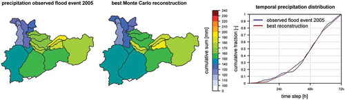
To assess whether the proposed method produces realistic precipitation distributions, the total amount of precipitation measured during the 2005 flood event (160 mm within 72 h) was redistributed by applying the procedure described above. Several of the 10 000 generated spatio-temporal distributions were close to the observed distribution in terms of the spatial as well as the temporal pattern. The comparison between the observed distribution and the best fit out of the 10 000 valid distributions is shown in Figure 6.

Figure 6. Observed spatial and temporal precipitation distributions of the 2005 flood event compared with the best reconstruction out of 10 000 valid generated distributions.

3.2.2 Determination of the runoff coefficients

The highest observed runoff coefficients of catchments within the Aare–Bern basin are close to 0.75 (Naef et al. 1986). According to Cerdan et al. (2004), the runoff coefficient generally decreases with increasing catchment size. As all of the catchments analysed by Naef et al. (1986) represent portions of the Aare–Bern basin, values above 0.75 are not expected for the entire basin. Because the source of this value is almost 30 years old (Naef et al. 1986), the annual peak flows from 1985 to 2012 of all gauged catchments were also checked using the available runoff series within the Aare basin. The results verified that the runoff coefficients were highly variable, as expected, but none of them exceeded 0.75. Norbiato et al. (2009) came to the same conclusions for several catchments at the southern edge of the Alps. In addition, Merz et al. (2006) showed that runoff coefficients larger than 0.8 only apply when snowmelt processes are involved. However, the maximum precipitation depends on the moisture-holding capacity of the air and thus on the air temperature. The precipitation thresholds calculated by Grebner and Roesch (1998) are associated with a relatively high temperature throughout the atmosphere, which is not expected to be possible during periods when snow is a crucial factor in runoff generation on basin scale. Therefore a runoff coefficient of 0.75 was chosen for the worst case.

3.2.3 Unit hydrographs

Following the procedure proposed by Dooge (1959), a unit hydrograph was calculated for each of the 13 catchments based on the highest ever measured event over the last 95 years, which took place in August 2005. Assuming the assigned precipitation in a catchment is uniformly distributed over space and time for each time step t_x, the precipitation was first multiplied by the runoff coefficient and then added to the baseflow, taking into account flow durations and the retention of the lakes. The calculation of the baseflow is based on a two-parameter algorithm by Boughton (1986) in accordance with the suggestion by Chapman (1999). Daily precipitation data were gathered from the RhiresD dataset (MeteoSwiss 2011) and disaggregated to hourly values using hourly data from stations located within the respective catchment. The discharge time series at the inflows of the two lakes and at the outflow of the catchment were obtained by the Federal Office for the Environment (FOEN). The model built according to the scheme in Figure 1 is based on these 13 calculated unit hydrographs.

3.2.4 Lakes

The two lakes located inside the catchment, Lake Brienz and Lake Thun, have a buffering effect on the total runoff; hence, they must be incorporated in the model. The hydrological behaviour of the two lakes is represented by nonlinear relations describing the relationship between the water level and discharge data provided by the Department for Water and Waste of the Canton of Bern (AWA). Both lakes can be regulated to a certain extent by weirs; therefore regulation affects the relationship between water level and discharge. To best replicate the worst-case scenario in the study area, parameters were set to represent fully open weirs, reflecting the maximum possible outflow for every possible lake level. Anthropogenic flood mitigation measures, such as intentional lowering of the lake level before a forecasted extreme event, are represented by applying the respective lake level.

3.2.5 Model performance

Data from the 2005 event (FOEN 2008) were used to develop the unit hydrographs, so it can be seen as the calibration event. The large flood events of 1987 (FOEN 1991) and 2007 (FOEN 2009) were used to validate to model. The runoff coefficients were adjusted according to the event-specific preconditions. This adjustment is reasonable as in this step only the shapes of the unit hydrographs are of importance, whereas the selected runoff coefficients in the model are not event specific but represent the worst case. Figure 7 shows the observed hydrographs of the three events as well as the hydrographs simulated with the observed precipitation pattern. To validate the model sensitivity to spatio-temporal precipitation distributions, the total event precipitation was redistributed by applying the proposed Monte Carlo algorithm and then fed into the model. The resulting variation of time and magnitude of peak discharge shows that the model reacts sensitively to spatio-temporal precipitation variation.

Figure 7. Measured and simulated hydrographs for the 2005, 2007 and 1987 events. The dashed line represents the model run with the observed precipitation data; the thin grey lines represent model runs with redistributed event precipitation and indicate the sensitivity of the model to the spatio-temporal precipitation distribution. The unit hydrographs were generated based on the 2005 event; hence it can be viewed as a calibration event.

For the calibrated 2005 event, the volume error is about 4%, where the discharge before the peak is overestimated and the discharge after the peak is underestimated. With regard to the two validation events, the volume error is about 5% for the 1987 event and about 4% for the 2007 event. Thus, the sum of the discharge is described with adequate accuracy. The peak discharge, which is even more important for the purpose of this study, is estimated well; the deviation in each case is below 5%. The Nash-Sutcliffe Efficiency criterion (NSE; Nash and Sutcliffe 1970) for the 2005 calibration event is 0.88, and it is 0.61 and 0.88 for the 1987 and 2007 validation events, respectively. The relatively low NSE for the 1987 event can be explained by the difference in process types between the 2005 calibration event and the 1987 event. The 2005 event, which was used to generate the unit hydrographs, was induced by 3 days of heavy rainfall on a saturated catchment (FOEN 2008). In contrast, the 1987 event was the consequence of relatively more persistent and less intensive continuous rainfall (FOEN 1991). This can be recognized clearly by viewing the measured hydrographs in Figure 7.

The 10⁴ physically plausible precipitation distributions mentioned in Section 2.2 were elicited for event durations of 48 and 72 h. A possible precipitation event lasting 47 or fewer hours is already included in the 48-h event duration in the form of a one-sided temporal distribution (e.g. the possibility that the bulk of the total precipitation amount would fall within the initial hours).

4 Results

The result is the distribution of possible peak discharges induced by the maximum precipitation input and, based on that, the identification of critical spatio-temporal precipitation distributions. The hydrographs created with the 10⁴ valid spatio-temporal distributions per event duration are shown in Figure 8. The right boxplot in Figure 9 shows the distribution of the corresponding peak discharges. For the applied spatio-temporal precipitation distribution over three meteorological regions and 13 catchments with event duration of 72 h, the median peak discharge amounts to 1140 m³ s⁻¹, and the highest generated peak is 1575 m³ s⁻¹. In the case of the 48-h event duration, the median peak discharge is 1160 m³ s⁻¹ and the highest generated peak is 1550 m³ s⁻¹ (not shown in the plot). The distribution of the peak discharges within this range depends on the spatio-temporal precipitation distribution.

Figure 8. Example of the generated hydrographs for the event duration of 72 h. The single hydrographs represent the various spatio-temporal precipitation distributions as discussed in Section 4.

Figure 9. Range of peak discharges of each modelled hydrograph compared with the FOEN (2009) results and the envelope curve by Weingartner (1999). The points indicate the highest ever observed events for the Aare–Bern basin as well as for smaller catchments within the basin. The boxplot to the far right represents the variation of catchment reactions to a given worst-case input due to varying spatio-temporal precipitation distributions.

The estimated values shown in Figure 9 are plausible compared to former estimations, although they are clearly higher due to the maximization of the total event precipitation. An envelope curve of the highest observed floods was estimated by Weingartner (1999). However, recent flood events exceeded this envelope curve, which shows that this curve must not be considered an upper limit. The study by FOEN (2009), which was carried out for a 2000-km² catchment within the Aare–Bern basin, is based on various precipitation scenarios. These scenarios were deduced from the highest observed flood event in 2005 by shifting and scaling the observed precipitation patterns. Considering that FOEN (2009) carried out their study on a smaller area of the catchment and applied a less maximizing approach based on observed events, the resulting model output is plausible. The spatio-temporal precipitation distributions that led to the peak discharges at the uppermost part of the resulting boxplot were identified as the most hazardous ones.

4.1 Spatial and temporal sensitivity

Model outputs with relatively high and low precipitation fractions of each catchment were analysed separately to evaluate the model sensitivity to spatial precipitation distribution. These high and low precipitation fractions were identified as those falling in the 0.01 and 0.99 percentiles of the event precipitation per catchment. The resulting boxplots are shown in Figure 10. The model sensitivity to the spatial precipitation distribution is mainly determined by the two lakes, which drain around 80% of the catchment area (meteorological regions A and B). In general, the model reacts more sensitively to the spatial precipitation distribution for the catchments that contribute directly to the runoff without traversing a lake (meteorological region C). The influence of catchments within a particular meteorological region is similar, whereas there is a relatively high variability of predicted peak discharge. To analyse the influence of temporal precipitation pattern on the model output, the events were divided into three categories based on temporal pattern and the according peak discharges were compared. Figure 11 shows that the applied model reacts sensitively to the temporal structure of the precipitation event. A higher peak discharge is modelled when the bulk of precipitation falls in the terminal phase of the event, which can be explained by the storage effect of the lakes. Overall, the influence of the temporal pattern on peak discharge is slightly smaller than the influence of the spatial pattern.

Figure 10. Range of the modelled peak discharges of model runs in which a particular catchment obtained an extremely high or low precipitation fraction. The peak discharge refers to the whole basin, e.g. the boxplot on the far left shows the distribution of the peak discharges of the whole basin resulting from all model runs in which the catchment A1 received a relatively high precipitation fraction.

Figure 11. Median peak discharges from model runs in which the temporal precipitation distribution was congruent with the respective sector.

5 Discussion

The benefit of this approach is its relative simplicity, and therefore its relatively good practical applicability to various catchments. It allows for many different plausible spatio-temporal precipitation distributions to be generated and validated in a relatively short time. The validation of the model in the case study with the 1987 and 2007 events showed that the catchment reaction can plausibly be reproduced. Therefore, the method can be applied to carry out a first estimation of discharge values of a hydrological worst-case scenario. The generation of a wide range of possible spatio-temporal precipitation distributions for a given total event precipitation enables an estimation of possible worst-case floods without using manually predefined distribution functions. This is clearly a benefit compared to standard precipitation generators (Leander et al. 2005, Furrer and Katz. 2008, Semenov 2008, Vandenberghe et al. 2010) or bootstrap techniques (Uboldi et al. 2014). Uncoupling the precipitation distribution from the parameters of observed events allows for consideration of a great variety of possible patterns. This also applies for the representation of variations in storm motions and storm velocities, which can also strongly influence subsequent PMF estimation (Seo et al. 2012, Nikolopoulos et al. 2014). Despite this uncoupling, some of the generated distributions are consistent with patterns often observed and correlations in space and time. Thus, the finally generated distribution of PMP is on one hand based on patterns similar to the ones observed, and on the other hand based on other physically plausible, but not yet observed patterns. In contrast, the stochastic storm transposition approach (Foufoula-Georgiou 1989, Franchini et al. 1996, Dodov and Foufoula-Georgiou 2005) primarily produces distributions that are similar to observed storm parameters and storm motions.

The main advantage of this method over resampling techniques (Paquet et al. 2013) and statistical description of storm structures (Salvadori and De Michele 2006, Langousis et al. 2013) is that the two steps of finding the worst-case flood causing precipitation distributions and implementing them in rainfall–runoff models are clearly separated. Therefore, the method ensures realistic conditions for the model input. Considering the fact that the applied hydrological model is not highly sophisticated due to the high number of model runs required, the result should be viewed as a rough estimation of the likely range of a PMF peak discharge. A subsequent application of sophisticated hydrological and hydraulic models allows for a more precise estimation in the consideration of step changes in runoff generation (Rogger et al. 2012b), variations in the initial conditions of the catchment, cryospheric influences on the runoff formation as well as catchment-specific event side effects such as landslides, inundations and log jams. In this case, the highest peak discharge is considered to be the PMF.

Care must be taken in communicating the findings of studies applying this method. The exploration of physical precipitation limits and the usage of maximal precipitation based on WMO (2009) to force this model lead to results that are much higher than common estimations such as those for events with return periods of 100 years. The maximal precipitation input is a theoretical construct and events with the estimated precipitation intensities may never occur. One must consider that this method is based on several assumptions about the model input that are not ultimately confirmable. The maximum precipitation amounts are also calculated on the basis of several theoretical assumptions, and their level of uncertainty is unknown. To account for uncertainties that influence PMP estimation, Micovic et al. (2015) recently proposed to replace single PMP values with ranges of possible PMP values. In the present study, PMP estimations from neighbouring regions were tested to take into consideration that the PMP estimations could be slightly different. This resulted in a slightly lower median (−8%) and in a lower maximum (−12%). The proposed method is applicable to catchments that are between 1000 and 10 000 km². If the catchment size is less than 1000 km², flood triggering processes on a catchment scale are more decisive than spatio-temporal precipitation distribution (e.g. persistent convective thunderstorms). If the catchment size exceeds 10 000 km², the superposition of different processes, the occurrence of independent precipitation events and the interplay among different processes become more important. However, this would also increase the calculation time of each model run and therefore negatively affect the applicability of the model to a Monte Carlo approach.

6 Conclusions and perspectives

By applying a simply built model, plausible spatio-temporal precipitation distributions that reveal high peak discharges can be generated by using a Monte Carlo approach. The scenarios generated by this method can be used as a foundation for more complex hydrological models than that used in this study. Besides identifying critical but realistic spatio-temporal precipitation distributions for further investigations, the method provides an estimation of the range of peak discharges that can be expected.

Finding an appropriate method for estimating peak discharge iteratively approaching the physical limit of a basin is still a challenge; at least for estimating system precipitation input and its spatio-temporal distribution, the present approach constitutes a step towards methodical reliability and allows the estimation to be based on different, varying methods, as proposed by Gutknecht et al. (2006).

Acknowledgements

The authors would like to thank the Federal Office for the Environment (FOEN), the Federal Office for Meteorology and Climatology (MeteoSwiss) and the Department for Water and Waste of the Canton of Bern (AWA) for providing the necessary input data. Anne de Chastonay, Fabia Hüsler, Ole Rössler and Bernhard Wehren are acknowledged for their thoughtful comments.

Disclosure statement

No potential conflict of interest was reported by the authors.

Additional information

Funding

This study is funded by the University of Bern and the Mobiliar Lab for Natural Risks.

References

- Beauchamp, J.R., et al., 2013. Estimation of the summer-fall PMP and PMF of a northern watershed under a changed climate. Water Resources Research, 49 (6), 3852–3862. doi:10.1002/wrcr.v49.6
- Boughton, W.C., 1986. Linear and curvilinear baseflow recessions. Journal of Hydrology (N.Z.), 25 (1), 41–48.
- Brandsma, T. and Buishand, A., 1998. Simulation of extreme precipitation in the Rhine basin by nearest-neighbour resampling. Hydrology and Earth System Sciences, 2 (2/3), 195–209. doi:10.5194/hess-2-195-1998
- Cerdan, O., et al., 2004. Scale effect on runoff from experimental plots to catchments in agricultural areas in Normandy. Journal of Hydrology, 299, 4–14. doi:10.1016/j.jhydrol.2004.02.017
- Chapman, T., 1999. A comparison of algorithms for stream flow recession and baseflow separation. Hydrological Processes, 13, 701–714. doi:10.1002/(ISSN)1099-1085
- Coles, S., 2004. An introduction to statistical modelling of extreme values. London, UK: Springer Press.
- Dodov, B. and Foufoula-Georgiou, E., 2005. Incorporating the spatio-temporal distribution of rainfall and basin geomorphology into nonlinear analyses of streamflow dynamics. Advances in Water Resources, 28, 711–728. doi:10.1016/j.advwatres.2004.12.013
- Dooge, J.C.I., 1959. A general theory of the unit hydrograph. Journal of Geophysical Research, 64 (2), 241–256. doi:10.1029/JZ064i002p00241
- FOEN (Federal Office for the Environment), 1991. Event-analysis of the 1987 flood. Report Nr. LHG-14-D. Bern, Switzerland.
- FOEN (Federal Office for the Environment), 2000. Flood 1999. Data Analysis and statistical classification. Report Nr. LHG-28-D. Bern, Switzerland.
- FOEN (Federal Office for the Environment), 2008. Event-analysis of the 2005 Flood. Part 2: Analysis of processes, measures and hazards. Report Nr. UW-0825-D. Bern, Switzerland.
- FOEN (Federal Office for the Environment), 2009. Event-analysis of the August 2007 Flood. Report Nr. UW-0927-D. Bern, Switzerland.
- Foufoula-Georgiou, E., 1989. A probabilistic storm transposition approach for estimating exceedance probabilities of extreme precipitation depths. Water Resources Research, 25 (5), 799–815. doi:10.1029/WR025i005p00799
- Franchini, M., et al., 1996. Stochastic storm transposition coupled with rainfall-runoff modeling for estimation of exceedance probabilities of design floods. Journal of Hydrology, 175, 511–532. doi:10.1016/S0022-1694(96)80022-9
- Furrer, E.M. and Katz, R.W., 2008. Improving the simulation of extreme precipitation events by stochastic weather generators. Water Resources Research, 44 (12). doi:10.1029/2008WR007316
- Grebner, D. and Roesch, T., 1998. Flächen-Mengen-Dauer-Beziehungen von Spitzenniederschlägen und mögliche Niederschlagsgrenzwerte in der Schweiz. Projektschlussbericht im Rahmen des Nationalen Forschungsprogrammes „Klimaänderungen und Naturkatastrophen“, NFP 31. Zurich: vdf Hochschulverlag.
- Gutknecht, D., et al., 2006. A „Multi-Pillar“-approach to the estimation of low probability design floods. Österreichische Wasser- und Abfallwirtschaft, 58 (3–4), 44–50. doi:10.1007/BF03165683
- Institute of Hydrology, 1999. Flood estimation handbook. Wallingford, UK: Institute of Hydrology.
- Koutsoyiannis, D., 1999. A probabilistic view of Hershfield’s method for estimating probable maximum precipitation. Water Resources Research, 35 (4), 1313–1322. doi:10.1029/1999WR900002
- Langousis, A., Carsteanu, A.A., and Deidda, R., 2013. A simple approximation to multifractal rainfall maxima using a generalized extreme value distribution model. Stochastic Environmental Research and Risk Assessment, 27, 1525–1531. doi:10.1007/s00477-013-0687-0
- Leander, R., et al., 2005. Estimation of extreme floods of the River Meuse using a stochastic weather generator and a rainfall-runoff model. Hydrological Sciences Journal, 50 (6), 1089–1103. doi:10.1623/hysj.2005.50.6.1089
- Matsumoto, M. and Nishimura, T., 1998. Mersenne twister: a 623-dimensionally equidistributed uniform pseudo-random number generator. Transactions on Modeling and Computer Simulation, 8 (1), 3–30. doi:10.1145/272991.272995
- McCuen, R.H., 2005. Hydrologic analysis and design. 3rd ed. Upper Saddle River, NJ: Pearson.
- Merz, R. and Blöschl, G., 2008. Flood frequency hydrology: 1. Temporal, spatial and causal expansion of information. Water Resources Research, 44 (8). doi:10.1029/2007WR006744
- Merz, R., Blöschl, G., and Parajka, J., 2006. Spatio-temporal variability of event runoff coefficients. Journal of Hydrology, 331, 591–604. doi:10.1016/j.jhydrol.2006.06.008
- MeteoSwiss, 2011. Documentation of MeteoSwiss Grid-Data Products. Daily Precipitation (final analysis): RhiresD. Available from: http://www.ifu.ethz.ch/hydrologie/research/research_data/proddocrhiresd.pdf [ Accessed 21 Apr 2015].
- Micovic, Z., Schaefer, M., and Taylor, G., 2015. Uncertainty analysis for Probable Maximum Precipitation estimates. Journal of Hydrology, 521, 360–373. doi:10.1016/j.jhydrol.2014.12.033
- Naef, F., Zuidema, P., and Kölla, E., 1986. Abschätzung von Hochwassern in kleinen Einzugsgebieten. In: M. Spreafico, ed.Beiträge zur Geologie der Schweiz – Hydrologie, Vol. 31. Bern, Switzerland: Swiss Geotechnical Commission, 195–233.
- Nash, J.E. and Sutcliffe, J.V., 1970. River flow forecasting through conceptual models part I — a discussion of principles. Journal of Hydrology, 10, 282–290. doi:10.1016/0022-1694(70)90255-6
- Nikolopoulos, E.I., et al., 2014. Catchment-scale storm velocity: quantification, scale dependence and effect on flood response. Hydrological Sciences Journal, 59 (7), 1363–1376. doi:10.1080/02626667.2014.923889
- Norbiato, D., et al., 2009. Controls on event runoff coefficients in the eastern Italian Alps. Journal of Hydrology, 375, 312–325. doi:10.1016/j.jhydrol.2009.06.044
- Papalexiou, S.M. and Koutsoyiannis, D., 2006. A probabilistic approach to the concept of Probable Maximum Precipitation. Advances in Geosciences, 7, 51–54. doi:10.5194/adgeo-7-51-2006
- Papalexiou, S.M., Koutsoyiannis, D., and Makropoulos, C., 2013. How extreme is extreme? An assessment of daily rainfall distribution tails. Hydrology and Earth System Sciences, 17, 851–862. doi:10.5194/hess-17-851-2013
- Paquet, E., et al., 2013. The SCHADEX method: A semi-continuous rainfall-runoff simulation for extreme flood estimation. Journal of Hydrology, 495, 23–37. doi:10.1016/j.jhydrol.2013.04.045
- Rogger, M., et al., 2012a. Runoff models and flood frequency statistics for design flood estimation in Austria – do they tell a consistent story? Journal of Hydrology, 456–457, 30–43. doi:10.1016/j.jhydrol.2012.05.068
- Rogger, M., et al., 2012b. Step changes in the flood frequency curve: process controls. Water Resources Research, 48 (5). doi:10.1029/2011WR011187
- Rössler, O., et al., 2014. Retrospective analysis of a nonforecasted rain-on-snow flood in the Alps – a matter of model limitations or unpredictable nature? Hydrology and Earth System Sciences, 18, 2265–2285. doi:10.5194/hess-18-2265-2014
- Salvadori, G. and De Michele, C., 2006. Statistical characterization of temporal structure of storms. Advances in Water Resources, 29, 827–842. doi:10.1016/j.advwatres.2005.07.013
- Schumann, A., 2007. Application of partial probability weighted moments to consider historical events in statistics of extreme. Hydrology and Water Resources Management, 51 (2), 73–81.
- Schumann, A., 2012. What is the return period of an extreme flood event if it is estimated to be many times higher than the HQ100? Hydrology and Water Resources Management, 56 (2), 78–82.
- Semenov, M.A., 2008. Simulation of extreme weather events by a stochastic weather generator. Climate Research, 35, 203–212. doi:10.3354/cr00731
- Seo, Y., Schmidt, A., and Sivapalan, M., 2012. Effect of storm movement on flood peaks: Analysis framework based on characteristic timescales. Water Resources Research, 48 (5). doi:10.1029/2011WR011761
- Uboldi, F., et al., 2014. A spatial bootstrap technique for parameter estimation of rainfall annual maxima distribution. Hydrology and Earth System Sciences, 18, 981–995. doi:10.5194/hess-18-981-2014
- Vandenberghe, S., et al., 2010. A stochastic design rainfall generator based on copulas and mass curves. Hydrology and Earth System Sciences, 14, 2429–2442. doi:10.5194/hess-14-2429-2010
- Verhoest, N.E.C., et al., 2010. Are stochastic point rainfall models able to preserve extreme flood statistics? Hydrological Processes, 24, 3439–3445. doi:10.1002/hyp.7867
- Wehren, B., 2010. The Hydrology of the Kander River – yesterday, today, tomorrow. Analysis and Modelling of the floods and their spatio-temporal dynamics. Thesis (PhD). University of Bern, Switzerland.
- Weingartner, R., 1999. Regionalhydrologische Analysen. Grundlagen und Anwendungen. Beiträge zur Hydrologie der Schweiz. Report Nr. 37. Bern, Switzerland.
- WMO (World Meteorological Organization), 1986. Manual for estimation of probable maximum precipitation. Operational Hydrology Reports 1, no. 332. 2nd ed. Geneva, Switzerland: WMO.
- WMO (World Meteorological Organization), 2009. Manual on Estimation of Probable Maximum Precipitation (PMP). Report no. 1045. WMO, Geneva, Switzerland.