Analysing individual recession events: sensitivity of parameter determination to the calculation procedure

ABSTRACT

This study assesses the sensitivity to model fitting methods and segment selection of the estimated parameters A and B of the model dQ/dt = −AQ^B for individual events. We investigated about 750 recession events observed at 25 US Geological Survey gauges in the Iowa and Cedar river basins in the United States, with drainage areas ranging from 7 to 17 000 km². The parameters of these recession events were estimated using three commonly adopted methods and recession segments with different extraction criteria. The results showed that the variations of the parameter estimates for the same recession event were comparable to the variations of parameters between different events due to using different model fitting methods and recession segments. This raises cautions for comparative analysis of individual recessions. The result also implies that the nonlinear direct fitting method is the most robust among the three model fitting methods compared.

EDITOR Z.W. Kundzewicz ASSOCIATE EDITOR T. Okruszko

KEYWORDS:

• Recession analysis
• recession variability
• recession parameters
• model fitting

1 Introduction

Quantitative analyses of recession curves require the selection of mathematical expressions and the determination of recession parameters. Among the mathematical models (e.g. Tallaksen 1995, Vogel and Kroll 1996, Moore 1997), the power-law function proposed by Brutsaert and Nieber (1977) has been widely adopted:

(1)

where dQ/dt is the time rate of change in streamflow Q, and A and B are model parameters. Parameters A and B are called the recession intercept and recession slope, respectively, in the plot of log(−dQ/dt) against log(Q), and represent two aspects of a recession event, i.e. the recession rate and the linearity of the storage vs discharge relationship, respectively. Examining the variability of recession behaviour, i.e. the variability of A and B across and within watersheds, has long been used to understand the functioning of watersheds (e.g. Vogel and Kroll 1992, Troch et al. 1993, Brutsaert and Lopez 1998, Szilagyi et al. 1998, Clark et al. 2009, Harman et al. 2009, Biswal and Marani 2010, Mutzner et al. 2013, Shaw et al. 2013). Interested readers should refer to the more comprehensive review articles (Tallaksen 1995, Smakhtin 2001, Troch et al. 2013). To increase the confidence of these inferences from studying recession variability, the sensitivity of parameter determination to the calculation procedure needs to be assessed (Rupp and Selker 2006a, Stoelzle et al. 2013).

The following terms are used in this paper. Segment selection means extracting portions of a recession curve with different starting points and lengths. Model fitting is the processes of finding the parameters A and B in Equation (1) by minimizing the differences between data and model predictions. The calculation procedure consists of segment selection and model fitting.

The parameters A and B are often determined using multiple recession events in the past. For example, Brutsaert and Nieber (1977) used the lower envelope; Vogel and Kroll (1992) employed the best regression line; and Kirchner (2009) used binned curve fitting of the dQ/dt−Q plot. These methods use dQ/dt−Q plots generated by mixing data points from many recession curves. However, the work of Biswal and Marani (2010) and Shaw and Riha (2012) argued that the model parameters were systematically biased when comparing individual recessions and multiple recession segments. They further suggested that examining and comparing individual event recession curves provides another way to explore hydrological processes. This approach gained attention in the past and is found increasingly in the recent literature (e.g. Vogel and Kroll 1996, Sujono et al. 2004, van de Giesen et al. 2005, Hammond and Han 2006, Blume et al. 2007, Rupp et al. 2009, Shaw et al. 2013, Biswal and Nagesh Kumar 2014, Chen and Krajewski 2015).

There is some flexibility in determining parameters A and B for individual recession events. To determine the parameters, many criteria for selecting recession segments and model fitting methods have been proposed, which causes arbitrariness in recession analysis. On the one hand, the recession segments used to calculate parameters A and B can be selected according to various criteria with different starting points and lengths (e.g. Aksoy and Wittenberg 2011, Brutsaert and Nieber 1977, Vogel and Kroll 1992, Tallaksen 1995, Kirchner 2009). On the other hand, parameters A and B in Equation (1) can be estimated using the log-log linear least squares fitting method employed by Vogel and Kroll (1992) and the nonlinear direct fitting method proposed by Wittenberg (1999). Furthermore, the calculation of dQ/dt can take either a fixed time step, which has been shown to be sensitive to the noise in the recession data (Kroll et al. 2004, Kirchner 2009), or variable time steps, as recommended by Rupp and Selker (2006a), to overcome this restriction.

The determination of parameters A and B for individual recession events may also be sensitive to the uncertainty in streamflow data. Streamflow data estimated by means of rating curves have substantial combined error, and this error can reach 100% for low flows (Harmel et al. 2006, McMillan et al. 2012). The US Geological Survey (USGS) often presents overall uncertainty in streamflow in a percentage fashion, while others may take the absolute measure (e.g. Kroll et al. 2004, Rupp and Selker 2006a, Shaw and Riha 2012, Thomas et al. 2013). To reduce the impact of the precision of streamflow data on the estimation of recession parameters, some strategies have been proposed to tackle this problem. For example, Rupp and Selker (2006a) suggested using a scaled time step to calculate dQ/dt; Kroll et al. (2004) and Thomas et al. (2013) recommended handling the noise in the original streamflow records by applying a moving average and using optimal smoothing splines techniques, respectively; and Kirchner (2009) pointed out the benefits of averaging out the noise in the calculated dQ/dt by binning. While all of these strategies are designed to smooth the data noise, limited efforts have been devoted to comparing the robustness of model fitting methods with respect to the uncertainty in streamflow data.

There seems to be a widely used functional form (Equation (1)) of the recession model, while many calculation procedures have been developed to determine the parameters A and B. The flexibility in determining model parameters leads to artificial recession variability and raises the question: Does the recession variability originate from physical processes or from inconsistent procedures used for data analysis? To exercise caution when interpreting and comparing the results of recession analyses, rather than providing new insights into the physical meaning of recession processes, this study aims to assess the sensitivity of the resulting model. dQ/dt = −AQ^B, for individual recession events with respect to:

1. the starting point and length used to extract segments from complete individual recession curves;

2. the model fitting method used to determine A and B; and

3. the noise in the recession data.

Specifically, we evaluate the performance of three methods (CTS, VTS and NDF) and investigate whether their estimates of A and B differ significantly. Monte Carlo simulations are used to examine the robustness of model fitting methods with respect to the noise in the streamflow.

2 Data and methods

This study contains several key definitions. A “complete recession curve” is the portion of a discharge hydrograph starting from the peak and extending to the point at which the hydrograph begins to increase. A “recession segment” refers to a portion of a complete recession curve (Tallaksen 1995, Sujono et al. 2004). Therefore, different recession segments can be extracted from the same complete recession curve by changing the starting point and the segment length. The “starting point” is the time elapsed since the occurrence of the hydrograph peak. These definitions apply to the true hydrograph, i.e. the actual discharge values. However, we only know the observed hydrograph, which is corrupted by errors. The data uncertainty issues will be addressed later in the paper. We use the recession slope B (see Equation (1)) as an example to demonstrate the sensitivity of its estimates with respect to the calculation procedure.

2.1 Data and study area

We analysed about 750 recession events observed over the period from 1995 to 2010 at 25 USGS stream gauges in the Iowa and Cedar river basins in Iowa, USA (Fig. 1). The corresponding drainage area at the gauge locations ranges from 7 to 17 000 km². These gauges are free from reservoir regulations and notable water withdrawals for agricultural or municipal use. The agricultural practices are rainfed, and the region has a small number of farm ponds. For this region, with rather flat terrain, approximately 75% of the 900 mm average annual precipitation and 85% of the 45–65 thunderstorms occur between April and September (Villarini et al. 2011). The annual evapotranspiration for this region is about 600 mm. Frozen soils and snow melting near the surface last from late October to early April. Water level is recorded every 15 or 30 minutes and is translated into discharge by applying the stage-discharge relation. We downloaded these sub-hourly streamflow data from the USGS Instantaneous Data Archive (http://ida.water.usgs.gov/ida/) and aggregated them to hourly time series. It is worth noting that the error structure of streamflow observations remains unknown (more details in Sections 2.4 and 3.5) and may deserve future investigation.

Figure 1. Location of the USGS stream gauges used in this study.

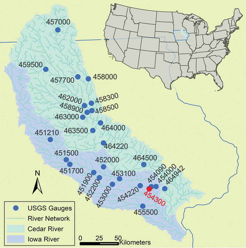
We show details of our analysis for the recession events observed at the Clear Creek stream gauge near Coralville, Iowa, USA (red dot in Fig. 1), and present summaries of our analysis for all of the gauges. Clear Creek is one of the US National Science Foundation’s critical zone observatories and is representative of the US Midwestern watersheds subject to agricultural land use and a humid climate. Clear Creek is an intensively instrumented and studied experimental watershed (Bradley et al. 2002, Abaci and Papanicolaou 2009, Rayburn and Schulte 2009, Loperfido et al. 2010, Risley et al. 2010, Berne and Krajewski 2013). This watershed drains an area of ~250 km² and has longest flow length of ~50 km. The time of concentration for this watershed is on the order of 1 day if the channel velocity is assumed to be 0.5 m/s. Land cover in this watershed is dominated by agricultural uses including corn, soybeans and pasture.

2.2 Selection of complete recession curves and recession segments

Considering the hydro-climatological characteristics of the region mentioned in Section 2.1, only summer and autumn recession events were analysed in this study. We used the following automatic algorithm to select recession curves. For each gauge, isolated events were selected from its continuous discharge hydrograph by applying a threshold, which was the estimate of the 95% quantile of hourly streamflow at the gauge. The times of peak discharge for each event were subsequently marked, and the hydrograph segments between two consecutive peaks (events) were extracted. For each of these selected segments, we identified a complete recession curve starting from the first hydrograph peak and extending until the difference between consecutive observations is greater than 0.1 mm/d. That is, if dQ = Q_t+1 − Q_t > 0.1 mm/d then a recession event stops at time t. Shaw and Riha (2012) estimated the USGS low flow measurements to have a precision of approximately 0.09 m³/s across basins, which is about 0.1 mm/d for a watershed of 100 km². We use this value as our threshold to account for spurious increases and “stair-step” patterns in low flow measurements. It is worth noting that the threshold is used to identify the end of a complete recession curve but not to set a “limiter” for dQ/dt. In this study, only complete recession curves longer than 10 days were considered.

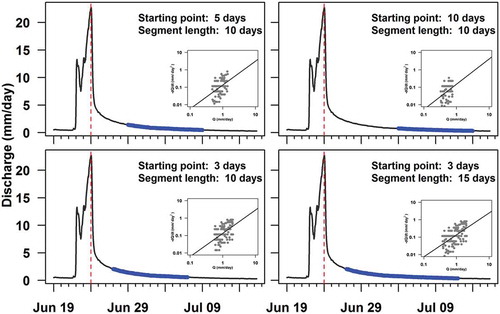
Figure 2 shows our approach to investigating how parameter determination depends on the selection of recession segments. Segments from a complete recession curve were extracted with various starting points and lengths. By taking the strategies illustrated in the upper and lower panels of Figure 2, we were able to investigate the dependence of B on the starting point and length of recession segments, respectively. This analysis was repeated for all hydrographs included in the study. When investigating how the estimation of B depends on the starting point, we varied the starting points from 0, 3, 6, 9, 12, 18, 24, 36, 48, 60, 72, 96, 120, 144 and 168 hours (7 days) after the hydrograph peak. When examining how the estimation of B depends on the recession length, we changed the recession lengths from 4, 5, 6,… up to 12 days if the recession was not interrupted by consecutive storms.

Figure 2. Schematic of selecting recession segments from a complete recession curve by fixing the length while varying the starting points (upper panels) and by fixing the starting point while varying the lengths (lower panels). The insets are the associated dQ/dt vs Q plots following the VTS method and the straight lines in these plots are the regression lines. The starting point of a recession segment is measured from the hydrograph peak marked by the red dashed line. The blue curve is the recession segment used to estimate the recession parameters A and B. This is a 27-day complete recession curve observed at Clear Creek near Coralville, Iowa (USGS 454300), for 24 June 2007 until 19 July 2007.

2.3 Model fitting methods

2.3.1 Constant time step method (CTS method)

The terms in Equation (1) can be discretized as dQ/dt = (Q_t − Q_t−1)/∆t and Q = (Q_t + Q_t-1)/2 for a given recession segment, where the time step ∆t is constant. The time step can be chosen to be 1 day (Brutsaert and Nieber 1977, Vogel and Kroll 1992, Biswal and Marani 2010), 1 hour (Clark et al. 2009, Kirchner 2009, Brauer et al. 2013), or 15 minutes (Rupp and Selker 2006a). For the constant time step method investigated in this study, we first calculated dQ/dt and Q for an individual recession event using a constant time step of 1 hour and then adopted the log-log simple linear least squares regression method used by Vogel and Kroll (1992) to determine A and B.

2.3.2 Variable time step method (VTS method)

Rupp and Selker (2006a) showed that the CTS method may bias the estimates of A and B, and they recommended the use of variable time steps to calculate dQ/dt in order to remove this limitation. For the VTS method compared in this paper, we first calculated dQ/dt and Q for an individual recession event using variable time steps and then adopted the log-log simple linear least squares regression method used by Vogel and Kroll (1992) to estimate A and B. To implement the VTS method (Rupp and Selker 2006a), the stage-discharge relationship and the stage measurement accuracy are required to determine the threshold C (C ≥ 0, Equation (15) in their paper) and thus ∆t. However, this information is often not available, and the value of C ends up being arbitrary. Palmroth et al. (2010) proposed using the criterion:

(2)

We followed this approach and set the value of C to be constant at 0.001 for all of our analyses, as Palmroth et al. (2010) did in their study.

2.3.3 Nonlinear direct fitting method (NDF method)

The third method is the nonlinear direct fitting method recommended by Wittenberg (1999). Accordingly, we varied B systematically, e.g. from 0 to 5 with a step size of 0.01, and calculated the value of A at each value of B using the equation:

(3)

where n is the length of the recession segment, and ∆t is the observational interval. Solving Equation (1) for Q_t gives:

(4)

where Q₀ is the discharge at the starting point of the recession segment used to calculate B, and t is the number of hours elapsed from the starting point. All recession segments are modelled using their initial discharges Q₀, the values of A and B, and Equation (4). The modelling error E is defined as:

(5)

where V_obs and V_mod are the volumes of flow of the observed and modelled hydrographs, respectively. The optimal paired values of A and B were selected by minimizing the modelling error.

2.3.4 Data points used by model fitting methods

After a recession segment is selected, the three methods are used to determine its recession parameters. To make log(−dQ/dt) valid, the CTS method requires the exclusion of non-negative dQ/dt values. This requirement is satisfied by eliminating the non-negative values after dQ/dt are calculated (Brutsaert 2008, Stoelzle et al. 2013). In the VTS method, the criterion (Equation (2)) automatically makes log(−dQ/dt) valid. When small C values are chosen, Equation (2) selects strictly monotonically decreasing data points for model fitting. The choice of the value of C determines the number of points used for model fitting. The NDF method uses all of the data points to estimate A and B. When applying these three methods, it is possible that different data points from the same recession segment are used in model fitting. However, these are the methods commonly used in the literature, and little attention is paid to how they may give notably different parameter values for the same recession event.

2.3.5 Comparison of the parameter estimates

Measure of variability due to segment selection: For each event at a gauge, recession segments are extracted from the complete recession curve with a fixed length but various starting points (Fig. 2, upper panel). Then, the associated estimates of B are obtained using the same model fitting method. Next, the range of B (defined as ) is calculated and used as a measure of the variation of B due to the change in starting points for the selected recession event. This analysis is repeated to obtain the values of ΔB for all recession events at each USGS gauge. A similar approach is used to calculate the variation of B due to the change in recession lengths.

Paired t-tests: For each basin we use the same criteria to extract recession segments (e.g. a starting point of 2 days after the hydrograph peak and a length of 7 days), then determine B values using the three methods, and finally conduct three paired t-tests of the estimates: CTS versus VTS, CTS versus NDF, and VTS versus NDF, to check whether these method give different results. These paired t-tests are repeated for all the 25 sub-basins in the Iowa and Cedar river basins.

Modelling error: Once the estimates of A and B are obtained for a given recession segment using the three methods described above, Equations (4) and (5) can be used to assess the goodness of fit. As in other works (Wittenberg 1999, Hammond and Han 2006), we assume that the method producing the smallest modelling error E outperforms the others.

2.4 Robustness with respect to uncertainty in streamflow data

Determining the robustness of the model fitting methods with respect to data errors is important because errors in the data may lead to biased estimates of parameters (Draper et al. 1966, Gupta and Dawdy 1995, Ciach and Krajewski 1999, Fuller 2006, Carroll et al. 2010). Streamflow data are subject to stage measurement and rating curve errors, surface–groundwater interactions, as well as evapotranspiration in the vicinity of streams. The uncertainty in streamflow data is usually described as a percentage of flow rates when assessing the quality of streamflow measurements (Harmel et al. 2006, McMillan et al. 2012) and modelling errors in streamflow measurements (Georgakakos 1986, Weerts and El Serafy 2006).

In this study, we used the Monte Carlo simulation method to assess the robustness of the model fitting methods with respect to the uncertainty in streamflow data. First, a noise-free (“true”) recession segment of 7-day length at an hourly time step (168 values) was generated. Then, for each run, the true curve was corrupted with a vector of noise with 168 elements, and the methods discussed in Section 2.3 were applied to estimate the parameters A and B. For each magnitude of noise, we ran 1000 simulations and took the mean and standard deviation of the estimates of A and B given by each of the methods. The means were compared to the true values that were used to generate the noise-free recession segment.

We generated the noise-free (“true”) recession segment based on our knowledge of the recession behaviour at the Clear Creek stream gauge near Coralville, Iowa. A visual examination of the complete recession curves at this gauge reveals that discharge usually drops below 2 mm/d two days after hydrograph peaks. Typical values of A and B at this gauge (See Section 3.5) were determined based on the analyses of the recession segments that start 2 days after a hydrograph peak with a length of 7 days. Thus, we created a 7-day long noise-free recession segment with an hourly time step using the power-law function dQ/dt = −AQ^B and an initial discharge of 2 mm/d.

The noise-free recession segment was corrupted by either multiplicative uncorrelated noise or multiplicative correlated noise. Errors in consecutive streamflow measurements have been assumed to be correlated (Kitanidis and Bras 1980, Sorooshian and Dracup 1980, Foglia et al. 2009) or uncorrelated (Georgakakos 1986, Weerts and El Serafy 2006) in the literature. We tested both cases in this study and introduced noise to the true recession segments data using:

(6)

where E(t) is the noise process, and Q(t) and Q_true(t) are the time-varying corrupted and noise-free recession segments. We generated vectors of uncorrelated noise from a normal distribution of N(0,σ) following Weerts and El Serafy (2006) and vectors of correlated noise using the first-order autoregressive model (Sorooshian and Dracup 1980):

(7)

where σ is the magnitude of noise, t = 1, 2, …, 168, ρ is the lag-one serial correlation coefficient for the errors and takes a positive value less than 1, and ε(t) is an i.i.d. random variable with mean 0 and standard deviation .

We estimated the levels of correlation of “noise” in observed recession data and used them in a Monte Carlo simulation study of the multiplicative correlated noise case. We first estimated the recession parameters for each of the observed recession events at Clear Creek using the NDF method and subsequently used the estimated A and B values to reproduce the associated recession segment. We then fitted AR(1) models to the residuals of the recession model for each of the events to obtain the associated values of ρ. We investigated different magnitudes of noise at σ = 1%, 3%, 5%, 8%, 10% and 15%.

3 Results

3.1 Variability due to choice of starting point

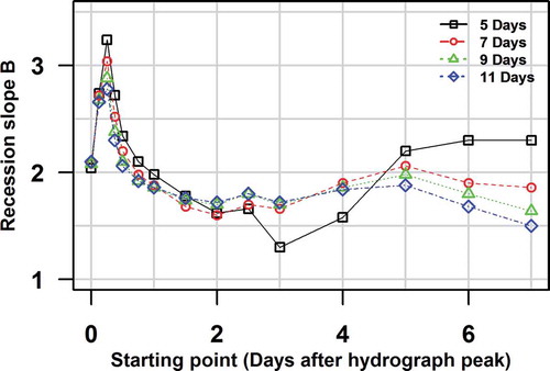
The analysis of a single event shows that the estimation of B varies substantially with the starting points of recession segments (Fig. 3). To show how the starting points of recession segments affect the estimation of B, we took a recession event observed at the Clear Creek stream gauge near Coralville, Iowa, as an example. The selected complete recession curve has a total length of 27 days from 24 June 2007 until 19 July 2007 (Fig. 2). At each fixed recession length, we first extracted recession segments using different starting points (0–7 days after hydrograph peak) and then estimated the values of B using the NDF method. Figure 3 shows that, for the same recession event, the estimates of B for its recession segments with the same length but different starting points can differ on the magnitude of 1.5.

Figure 3. Variability of B estimates due to the change in starting point of recession segments (a single event). The same example recession event as in Figure 2 is used here. Key shows length of recession segments used to estimate B.

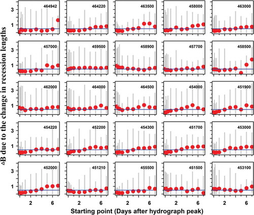
Analyses of all of the recession events selected in this study also show a high variation of the B estimates due to the change in the starting points of recession segments. Figure 4 shows that ΔB, i.e. the variation of B due to the change in starting points at each fixed length, can take values ranging from 0 to 3. The median values of ΔB (red dots in Fig. 4) for all gauges are around 1. Similar results (not shown) were obtained when repeating similar analyses using the CTS and VTS methods. Precautions should be taken when using A and B to characterize individual recession behaviour because the estimation of A and B is sensitive to the starting point of the recession segment.

Figure 4. Variability of B estimates due to the change in starting points of recession segments (multiple events). For each USGS gauge (see gauge ID at the top right corner), we repeated the analysis in Figure 3 to obtain ΔB values for all of the recession events. Each red dot is the median value and each grey line segment represents the range of ΔB at a fixed recession length. The median values of ΔB for all gauges are around 1.0.

3.2 Variability due to choice of recession length

The analysis of a single event shows that the estimation of B tends to be affected by the lengths of recession segments (Fig. 5). The same recession event, as described in Section 3.1, was used to investigate the dependence of B on the lengths of recession segments. At each fixed starting point, we first extracted recession segments using different lengths (4–12 days) and then estimated the values of B using the NDF method. Figure 5 shows that, for the same complete recession curve, the estimates of B for its recession segments with the same starting point but different lengths can vary on the magnitude of 0.5.

Figure 5. Variability of B estimates due to the change in length of recession segments (a single event). The same example recession event as in Figure 2 is used here. The text at the top right corner is the starting point (number of days after hydrograph peak) of the recession segments used to estimate B.

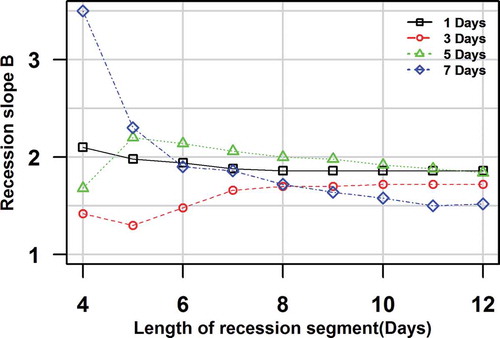
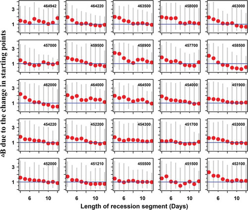
Analyses of all of the recession events selected in this study also show that the B estimates tend to vary greatly with the lengths of recession segments. Figure 6 shows that ΔB, i.e. the variation of B due to the change in recession length at each fixed starting point, can take values ranging from 0 to 2 (for most gauges). The median values of ΔB (red dots in Fig. 6) for all gauges are around 0.5. Similar results (not shown) were obtained when repeating similar analysis using the CTS and VTS methods. One must be cautious when comparing the A and B values for different events, especially if the difference in the lengths of the two recession segments used to estimate A and B is large.

Figure 6. Variability of B estimates due to the change in length of recession segments (multiple events). For each USGS gauge (see gauge ID at the top right corner), we repeated the analysis in Figure 5 to obtain ΔB values for all of the recession events. Each red dot is the median value and each grey line segment represents the range of ΔB at a fixed starting point. The median values of ΔB for all gauges are around 0.5.

3.3 Variability due to choice of model fitting methods

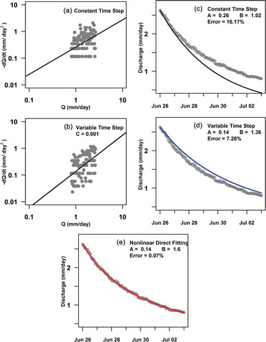
The analysis of a single event shows considerable differences among the values of B that were estimated by different methods (Fig. 7). A recession segment was extracted from the same recession event, as described in Section 3.1, with a starting point of 2 days after the hydrograph peak and a length of 7 days. This segment and the three model fitting methods introduced in Section 2.3 were used to estimate the value of B. For the VTS method, the value C = 0.001 was used to reduce the impact of the noise in streamflow data on the estimation of recession parameters. The modelling error was calculated as the relative difference between the volumes of modelled and observed recession flows. Figure 7 shows that the parameters estimated by the NDF method are most effective (smallest modelling error) in terms of reproducing the given recession segment. Surprisingly, the differences among the values of B estimated by these methods can be as high as ~0.6.

Figure 7. Variability of parameter estimates due to method choices. The same example recession event as in Figure 2 is used here. The parameters for the selected segment were estimated using the CTS (a) and (c), VTS (b) and (d) and NDF (e) methods. In (b), (d) and (e), open circles are measured streamflow values, and lines are the modelled recession segments using the estimated parameters.

For Clear Creek, the paired t-test shows that the values of B estimated by the three methods are statistically different. Comparisons between the parameters determined and the performances of the three methods are given in Table 1. These 30 recession segments were extracted from 30 recession events observed at the stream gauge near Coralville using a starting point of 2 days after the hydrograph peak and a length of 7 days. Paired t-tests showed that the estimates of B given by the three methods were different from each other at the significance level of p = 0.05. Furthermore, for at least 17 out of the 25 gauges investigated, the paired t-tests indicated that the B estimates given by the three methods were statistically different at the significance level of p = 0.05 (Table 2). This significant difference suggests that it would be wise to ensure that recession parameters are estimated using the same method when comparing them across events.

Table 1. Comparison of estimates of recession parameters A and B at Clear Creek near Coralville, Iowa (USGS 454300), calculated using the CTS, VTS and NDF methods. All recession segments have a starting point of 2 days and a length of 7 days.

Starting date	A			B			Modelling error (%)
Year/month/day	CTS	VTS	NDF	CTS	VTS	NDF	CTS	VTS	NDF
1995/07/06	0.22	0.19	0.20	0.30	1.41	1.94	54.63	9.82	0.41
1996/06/07	0.18	0.14	0.11	1.05	0.68	1.04	18.50	4.04	0.53
1997/05/08	0.20	0.16	0.21	0.42	1.20	2.08	41.51	5.71	0.68
1997/05/26	0.20	0.15	0.15	0.32	0.98	1.48	17.06	0.58	0.13
1998/10/05	0.26	0.13	0.13	1.42	2.17	2.52	15.49	3.38	0.51
1998/11/10	0.16	0.09	0.06	0.86	1.42	2.32	19.02	3.96	0.07
1999/04/23	0.17	0.06	0.06	1.13	2.32	1.84	21.00	5.66	0.23
2000/06/15	0.29	0.16	0.14	0.72	1.26	2.24	29.07	0.67	0.42
2000/07/10	0.32	0.18	0.18	1.13	1.76	2.08	29.54	0.17	0.96
2001/06/14	0.30	0.08	0.07	0.59	2.55	3.04	29.67	0.12	0.75
2001/10/23	0.29	0.53	1.48	0.54	1.92	3.78	47.87	11.45	3.49
2002/04/28	0.18	0.15	0.13	0.56	1.77	1.92	27.03	5.54	0.17
2002/08/23	0.30	1.33	1.84	0.37	2.23	2.54	60.57	3.31	0.40
2002/10/04	0.25	0.55	0.89	0.41	2.83	3.68	50.61	2.74	0.50
2004/05/31	0.21	0.13	0.12	1.23	1.66	2.12	20.19	2.82	0.46
2005/04/12	0.22	0.14	0.14	1.03	2.20	3.02	25.59	3.59	0.18
2007/04/13	0.17	0.12	0.09	0.88	1.92	2.92	18.31	5.45	0.77
2007/05/07	0.16	0.11	0.09	1.17	1.74	2.66	10.08	1.23	0.18
2007/06/24	0.26	0.14	0.14	1.02	1.36	1.60	16.17	7.28	0.07
2007/08/24	0.22	0.14	0.14	1.14	1.87	2.18	3.70	3.55	0.44
2007/10/02	0.23	0.22	0.24	0.31	3.00	3.72	37.19	1.92	0.11
2007/10/18	0.24	0.08	0.08	0.81	2.15	2.32	10.67	3.96	0.77
2008/07/22	0.27	0.10	0.09	0.69	1.46	1.66	23.47	0.41	0.16
2008/09/29	0.35	0.24	0.17	2.37	3.90	4.00	25.82	4.43	1.25
2009/06/24	0.10	0.08	0.08	1.70	2.15	2.20	1.47	3.16	0.06
2009/07/11	0.10	0.08	0.09	1.87	2.13	2.20	3.43	4.27	0.03
2009/07/25	0.13	0.13	0.15	0.49	1.83	2.64	16.19	2.51	0.18
2009/08/28	0.09	0.07	0.08	1.85	2.13	2.12	2.43	2.95	0.24
2009/10/30	0.04	0.04	0.03	2.30	2.54	2.80	2.21	3.01	0.25
2010/08/21	0.14	0.12	0.13	0.89	1.94	2.74	12.66	2.25	0.03
Median	0.21	0.14	0.13	0.88	1.92	2.28	19.61	3.35	0.33
Interquartile range	0.10	0.07	0.08	0.62	0.69	0.71	16.06	2.08	0.36

Table 2. Comparison of the estimates of B at 25 gauges calculated with the CTS, VTS and NDF methods. All gauges are located within the HUC05 of the United States, and we use only the last six digits of their complete USGS gauge ID. NRec is the number of recession events analysed; Medians of B are the median values of B for multiple events at a gauge; IQR of B is the interquartile range of B estimates for multiple events at a gauge; modelling error (%) is the median of the relative differences between the volumes of modelled and observed recession flows; p value is for the paired t-test; and ∆B is the median value of absolute difference of B estimates given by two methods.

USGS Gauge No.	Area (km^2)	NRec	Median of B			IQR of B			Modelling error (%)			p-value			∆B
			CTS	VTS	NDF	CTS	VTS	NDF	CTS	VTS	NDF	CTS-VTS	CTS- NDF	VTS- NDF	CTS-VTS	CTS- NDF	VTS- NDF
464942	7	14	0.55	1.31	2.06	0.80	0.88	0.70	31.21	11.39	0.83	0.15	0.01	0.00	1.31	1.75	0.76
464220	774	21	1.39	2.42	2.72	0.86	0.77	0.40	8.63	1.78	0.26	0.00	0.00	0.00	1.09	1.44	0.22
463500	784	18	2.03	2.38	2.63	0.73	0.71	0.82	0.69	0.87	0.39	0.00	0.00	0.00	0.32	0.62	0.20
458000	792	25	1.73	2.14	2.24	1.12	0.99	0.66	4.34	2.10	0.62	0.00	0.00	0.28	0.48	0.43	0.23
463000	898	30	1.78	2.20	2.48	1.09	0.75	1.02	1.25	1.19	0.56	0.00	0.00	0.01	0.33	0.41	0.23
457000	1033	12	1.45	1.96	1.89	0.30	0.77	1.18	4.15	1.32	0.26	0.00	0.00	0.05	0.55	0.62	0.24
459500	1362	38	1.19	1.45	1.62	0.81	0.85	1.17	4.03	1.26	0.37	0.02	0.00	0.01	0.26	0.58	0.15
458900	2190	24	1.93	2.27	2.13	0.94	1.29	1.43	1.96	1.38	0.87	0.00	0.00	0.45	0.16	0.39	0.20
457700	2729	22	1.47	1.65	2.08	0.70	1.05	1.43	8.21	3.19	0.52	0.00	0.01	0.25	0.37	0.68	0.27
458500	4300	13	1.76	1.82	2.14	0.82	0.62	0.90	1.76	1.19	0.31	0.00	0.00	0.20	0.53	0.74	0.23
462000	4520	33	1.19	1.59	1.66	0.62	0.63	0.84	1.60	0.83	0.24	0.00	0.00	0.25	0.23	0.33	0.13
464000	13322	25	1.77	2.04	2.22	0.68	0.64	0.48	2.60	0.88	0.59	0.00	0.00	0.00	0.31	0.54	0.30
464500	16854	9	1.54	1.67	2.18	1.15	1.23	1.54	5.60	1.42	0.30	0.07	0.06	0.08	0.47	0.98	0.51
454000	66	41	0.32	1.42	2.16	0.38	0.46	0.80	24.66	10.03	0.61	0.00	0.00	0.00	1.13	1.82	0.76
451900	145	41	0.73	2.11	2.70	0.48	0.90	0.90	29.52	5.51	0.45	0.00	0.00	0.00	1.31	1.85	0.64
454220	151	30	0.98	1.84	2.37	0.41	0.28	0.86	21.73	2.88	0.26	0.00	0.00	0.00	0.85	1.35	0.49
452200	184	35	0.67	1.51	2.14	0.49	0.39	0.69	28.45	4.36	0.40	0.00	0.00	0.00	0.81	1.47	0.62
454300	254	30	0.88	1.92	2.28	0.62	0.69	0.71	19.61	3.35	0.33	0.00	0.00	0.00	1.04	1.49	0.53
451700	306	25	1.21	1.96	2.62	0.52	0.48	0.88	7.31	2.43	0.61	0.00	0.00	0.00	0.66	1.36	0.69
453000	489	39	1.13	2.17	2.62	0.77	0.86	0.99	18.93	1.98	0.62	0.00	0.00	0.00	0.78	1.18	0.38
452000	520	31	1.63	2.45	2.82	0.85	0.52	0.80	6.65	0.94	0.29	0.00	0.00	0.00	0.73	1.34	0.46
451210	580	34	1.47	2.03	2.20	0.58	0.55	0.75	10.55	1.77	0.56	0.00	0.00	0.00	0.45	0.69	0.18
455500	1486	43	1.74	2.07	2.14	0.43	0.37	0.60	2.00	1.56	0.72	0.00	0.00	0.00	0.22	0.35	0.14
451500	3966	21	1.20	1.56	1.46	0.58	0.75	0.78	2.54	1.58	0.53	0.00	0.02	0.58	0.29	0.33	0.20
453100	7233	21	1.75	2.17	2.18	0.91	0.80	1.18	1.04	1.16	0.57	0.01	0.22	0.23	0.17	0.30	0.20

In summary, the artificial variability of B resulting from the calculation procedure is comparable to the variability of B among individual recession events. For the Clear Creek watershed, Table 1 shows that the variability of B among 30 individual recession events measured by interquartile range is about 0.7. Table 1 also shows that for individual events the differences between estimates of B given by the three methods can vary from 0 to ~1. For multiple watersheds, Table 2 shows that the variability of B among individual recession events is around 0.8 (median value), and the difference caused by the method of choice is about 0.3 (median value). Additionally, as we reported in Sections 3.1 and 3.2, the differences in the estimates of B for the same recession events are 1.0 and 0.5 due to changes in the starting points and lengths used to extract recession segments, respectively. These numbers suggest that when interpreting the temporal variability in the recession behaviour (e.g. represented by A and B) of a watershed, it is important to reduce the variability in the recession parameters caused by the processes of recession segment selection and model fitting.

3.4 Performances of the three model fitting methods

Data analyses shows that the NDF method tends to outperform the CTS and the VTS model fitting methods. For the majority of the ~750 recession events investigated, the given recession segments were reproduced with increasing magnitude of error by the parameters that were determined by the NDF, the VTS and the CTS methods (Table 2). This is consistent with the result of analysing the example event (Fig. 7). We found that the NDF method produces more reliable estimates of A and B at the expense of requiring a slightly longer computational time (<1 s) for a single recession event.

3.5 Effect of uncertainties in streamflow

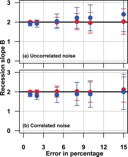
Analyses of observed recession data (from 30 events) in Clear Creek provide the inputs for the Monte Carlo simulation designed to test the robustness of the model fitting methods to data noise. Table 1 shows that the typical values of A and B at this gauge are around 0.15 and 2.0, respectively. These values were used to generate a noise-free (“true”) recession segment with an hourly time step using the power-law function dQ/dt = −0.15Q^2.0 and an initial discharge of 2 mm/d. Fitting AR(1) models to the residuals of the recession model for each of the events showed that the estimated values of ρ vary between 0.3 and 0.8, with a median value of around 0.6. Accordingly, we used six levels of correlation, ρ = 0.3, 0.4, 0.5, 0.6, 0.7 and 0.8 to generate the correlated noise.

Among the noise processes we investigated, the NDF method is more robust with respect to data errors and thus is preferred for model fitting. Figure 8 shows the mean and standard deviation obtained based on the results of 1000 simulations. The length of the recession segment used is 7 days (168 hourly flow values). The uncorrelated noise values are generated from a normal distribution N(0,σ). The correlated noise values are generated from the AR(1) model E(t) = ρE(t − 1) + ε(t), where ρ is the correlation coefficient (ρ = 0.6 for this figure), ε(t) is an i.i.d. random variable with mean 0 and standard deviation, and σ is the magnitude of data noise in percentage. The mean values of the estimates of B given by the NDF method (red dots) are close to the true value of 2.0 regardless of the existence of correlation in and the magnitude of the data noise. In contrast, the mean values of the estimates of B given by the VTS method (blue dots) tend to deviate from 2.0 as the magnitude of uncorrelated error increases. Furthermore, at each magnitude of the noise, the NDF method gives less variable estimates of B, indicating that it is more robust with respect to the noise in the recession data. As anticipated, for both methods, the estimation of B deteriorates as the magnitude of uncertainty in recession data increases. For the correlated error case shown in Figure 8, we contaminated the noise-free recession curve with noise correlated at the level of ρ = 0.6. We tested six levels of correlation, ρ = 0.3, 0.4, 0.5, 0.6, 0.7 and 0.8, and found results that are similar. We repeated the analysis for recession segments with lengths of 3, 5, 7 and 9 days and obtained similar results, except that longer segments tend to reduce the variance of the B estimates. Recall that the CTS method is most vulnerable to data noise, and therefore was not included in this comparison.

Figure 8. Robustness of the VTS (blue) and the NDF (red) methods with respect to the noise in streamflow data. The true value of B is 2. Filled circles represent the mean values of B. Error bars show the standard deviation of B estimates at each magnitude of error.

4 Discussion

Recession analysis has long been used to deepen our understanding of the functioning of watersheds. One avenue is to conduct comparative data analysis of recession characteristics across watersheds. The recession characteristic of a watershed is notionally derived by using multiple recession events collectively, indicating that the between-event variability for each watershed is neglected. As a complement to this avenue, conducting comparative data analysis across recession events from each watershed has gained increasing momentum in the recent literature. This second approach examines individual recession events and therefore emphasizes the between-event variability. Many quantitative recession analysis methods have been proposed. It is a necessity to assess the magnitude of discrepancies in the resulting recession models (e.g. recession parameters) given by different analysis methods. This will help to reduce the artificial variability due to data analysis and to make more confident inferences about physically driven factors of the observed recession variability. Stoelzle et al. (2013) have assessed the variation of the derived recession parameters due to calculation procedures for the case of examining multiple recession events collectively. As a derivative of their work, we designed this study to assess the sensitivity of the resulting model dQ/dt = −AQ^B for individual recession events with respect to the selection of recession segments and the model fitting method used to determine A and B. For this purpose, we analysed ~750 recession events observed at 25 sub-watersheds in the Iowa and Cedar river basins in the United States, with drainage areas ranging from 7 to 17 000 km².

4.1 Artificial variability can blur the natural variability of recession behaviour

The recession slopes B determined for individual events in this study are in the range of the values reported in the literature. Tables 1 and 2 show that recession slope B ranged from about 1 to 4 according to the values derived by the NDF method. This is consistent with the range of [1.3, 5.3] reported by Shaw and Riha (2012), the range of [1.0, 4.0] from Biswal and Marani (2010), the range of <1 to >3 reported by Tague and Grant (2004), and that B can be 3 at the early stages of recession and range from 1 to 2 for later stages (e.g. Brutsaert and Nieber 1977, Rupp and Selker 2006b). For all of these studies, the majority of the recession slopes B are within the range of [1.5, 2.5], though the full ranges are often wider. These previous studies indicate that the variability of the recession slope is about 1.0, and this is often attributed to the variations of natural processes or watershed properties. Table 2 in this study shows that the variability of B among individual recession events is around 0.8 (median value).

The results of data analysis presented in Section 3 suggest that the resulting recession models for individual events are sensitive with respect to the selection of recession segments and the choice of model fitting methods. For the same example recession event (Fig. 2), notable differences in the estimates of recession parameters can arise solely from the selection of segments (Figs. 3 and 5). For multiple recession events, the statistics reported in Sections 3.1 and 3.2 show that the differences in the estimates of B for the same recession events are 1.0 (Fig. 4) and 0.5 (Fig. 6) due to changes in the starting points and lengths used to extract recession segments, respectively. This confirms the notion that the estimates of recession parameters depend on the starting points (e.g. Vogel and Kroll 1992, Tallaksen 1995, Hammond and Han 2006) and lengths (Vogel and Kroll 1996) used to select recession segments. Additionally, Table 2 shows that the difference in the estimates of B caused by the method of choice is about 0.3 (median value), which is consistent with the literature (Vogel and Kroll 1996, Wittenberg 1999, Rupp and Selker 2006a, Stoelzle et al. 2013). These high sensitivities are not a surprise, knowing that Stoelzle et al. (2013) found considerable differences between the average recession characteristics (represented by A and B) obtained for the same watershed using different methods of segment selection and parameter determination. These average recession characteristics were derived using multiple events. Compared to the recession analysis using multiple recession events, individual recession analysis may be even more sensitive to the calculation procedure since, by definition, less information is available.

The quantitative sensitivity analyses discussed above show that the artificial variability of B resulting from the calculation procedure is notable when compared to the variability of B among individual recession events. Numerous studies have unveiled various natural causes of recession variability, to name a few but not limited to: the vertical heterogeneity of hydraulic conductivity (Troch et al. 1993, Rupp and Selker 2006b), the horizontal heterogeneity recession processes across hillslopes (Harman et al. 2009), landscape organization (e.g. Clark et al. 2009, Chen and Krajewski 2015), the shrinkage of the feeding river network or area to streamflow (Biswal and Marani 2010, Mutzner et al. 2013, Biswal and Nagesh Kumar 2014), and watershed moisture storage (Shaw et al. 2013). These studies have greatly advanced our knowledge of the hydrological functioning of catchments. It is worth noting that our sensitivity assessment implies that the natural variability of recession parameters can be blurred by the artifacts of recession data analysis. We did not mean to dispute the invaluable knowledge gained from recession analyses conducted by our respected predecessors. We are trying to show that the variability in the recession behaviour (e.g. represented by recession parameters A and B) of a watershed can originate from natural processes and the procedures of recession data analyses, and the latter need to be assessed and to be reduced (or even minimized if achievable, but this is difficult). This cautionary note should be beneficial to increase the fidelity of results drawn from future comparative recession analyses.

4.2 Recommendations for analysing individual recession curves

It is difficult to set up a concrete standard for examining individual recession curves, given the fact that recession behaviour is affected by the size, rainfall and drainage history, geology, human activities, and many other factors of a watershed. We hope that, together with other works (e.g. Vogel and Kroll 1992, Biswal and Marani 2010, Shaw and Riha 2012, Thomas et al. 2015), the lessons learnt from our more focused and systematic investigation can raise caution about the techniques used for analysing individual recession events.

It would be wise to consider using a consistent approach to select recession segments to examine the variability of individual recession events. It is widely accepted that the determination of recession parameters depends on the starting point of a recession segment (e.g. Brutsaert and Nieber 1977, Vogel and Kroll 1992, Tallaksen 1995). This is because the recession process is conceptualized as a mixture of drainage from various sources (Tallaksen 1995, Vogel and Kroll 1996, Szilagyi and Parlange 1998). Less attention has been paid to the impact of recession length on the determination of recession parameters (Vogel and Kroll 1996, Hammond and Han 2006). Our investigation shows that recession length can also moderately affect the determination of recession parameters. Therefore, at least within each study, using consistent starting point and recession length criteria to extract segments for recession analysis is suggested.

The nonlinear direct fitting (NDF) method is recommended for analysing individual recession events, especially when high temporal resolution flow data are used. While it is difficult to avoid uncertainty in streamflow data, we can assess the robustness of the model fitting methods with respect to data noise. Streamflow data estimated by means of rating curves have substantial combined error, and this error can reach 100% for low flows (Harmel et al. 2006, McMillan et al. 2012). Our data analyses (Tables 1 and 2) show that the NDF method produced smaller modelling errors compared to the constant time step (CTS) and the variable time step (VTS) methods. Furthermore, our data analyses (Fig. 7) and Monte Carlo simulation (Fig. 8) both indicate that the NDF method is most data noise resistant. Figures 7 and 8 also show that the noise in flow data deteriorates the estimation of the recession parameters and contributes to the differences between the recession parameters determined by different model fitting methods. This result agrees with those reported by Rupp and Selker (2006a), Kroll et al. (2004), Kirchner (2009) and Thomas et al. (2015) that reducing the impact with data noise is necessary for recession analysis.

The inherent features of the model fitting methods may explain why the NDF method performs better. On the one hand, both the CTS and the VTS methods estimate A and B on the log-log scale using least squares linear regression, with the goal of maximizing the amount of variation in log(−dQ/dt) rather than the variation in −dQ/dt that is explained by the power-law recession models. In contrast, the NDF method uses iterative direct curve fitting to estimate A and B in the original units. This leads to different optimal solutions for A and B. On the other hand, the CTS and the VTS methods calculate −dQ/dt using forward or backward differences, which are subject to numerical errors. This indicates that the estimates of A and B given by these two methods may be sensitive to the local noise in the recession data. In contrast, the NDF method estimates the parameters using an integrated approach (Equation (3)), which makes the estimation more robust with respect to local errors in the recession data due to the smoothing effect.

Recession analysis can be done using sub-daily and daily flow data, and this raises the question “what is the optimal time step for recession analysis?”. The optimal choice of the time step ∆t is determined from consideration of the drainage process of interest, the observational frequency, and the magnitude of noise of streamflow data. Using a small ∆t may suffer from the noise in the streamflow data, i.e. ∆Q = (Q_t − Q_t-∆t) may become comparable to the magnitude of data uncertainty, while choosing a large ∆t may lose the ability to capture the temporal evolution of the different drainage processes for a single recession event. Balancing this dilemma is difficult; for example, analysing recession data with high observational frequency (sub-daily scale) has its own value (e.g. Rupp and Selker 2006a, Clark et al. 2009, Kirchner 2009, Krakauer and Temimi 2011, Brauer et al. 2013) and we still have to deal with data noise even when using daily data (e.g. Palmroth et al. 2010, Chen and Krajewski 2015). Two methods can be used to tackle this problem: (1) using a shorter time step for the early stages and a longer time step for the late stages of the recession process (variable ∆t); and (2) using a method that is not sensitive the choice of ∆t.

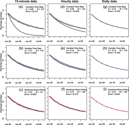
In this study, for the CTS method we used Δt = 1 h, for the VTS method there was no fixed Δt and for the NDF method Δt = 1 h. One might argue that if we use daily data, there would not be such a big difference between the parameters determined by the three methods. The same recession event used in Figure 7 is used here to illustrate the sensitivity of recession analysis to the choice of ∆t. We estimated the recession parameters A and B using the CTS, VTS and NDF methods and Δt = 15 min, 1 h and 1 day, respectively. Comparison shows that the NDF method is not sensitive to the choice of time step ∆t (Fig. 9). Consistent with the literature, our results indicate that the CTS method is most sensitive to the choice of time step (e.g. Rupp and Selker 2006a, Palmroth et al. 2010, Thomas et al. 2015) and the VTS method greatly reduces this sensitivity. Interestingly, the estimates given by the NDF method are almost identical when data with different temporal resolutions are used. Furthermore, the differences in the parameter estimates decrease with the degradation of the temporal resolution of streamflow data and are negligible at the daily scale. The similar values of A and B shown in the bottom and rightmost panels indicate that the NDF method is the most capable among the three to deal with data noise, allowing analysis of both the early- and the late-time recession data with high temporal resolution. The VTS method can also be used for this purpose, while more information is needed to determine the threshold value C (Rupp and Selker 2006a, Palmroth et al. 2010). Lastly, as pointed out by one of our reviewers, the recession parameters estimated by the CTS method for daily data (A = 0.13 and B = 1.76) are quite similar to the parameters estimated by NDF method for hourly data for the same period (A = 0.14 and B = 1.6, Fig. 9). This means that one can convert hourly data into daily data and apply the CTS method to obtain recession parameters and use them to recreate the hourly recession curve.

Figure 9. Comparison of A and B estimated using three methods and streamflow data with three temporal resolutions (dt = 15 min, 1 h, and 1 day were used to calculate dQ/dt). The same example recession event as in Figure 2 is used here. We extracted the recession segment from the complete recession curve using a starting point of 2 days and a length of 7 days. The open circles are the observed streamflow values, and the lines are the modelled recession segments using the estimated parameters. For the VTS method, the value C = 0.001 was used to reduce the impact of the noise in streamflow data on the estimation of recession parameters.

4.3 Limitations of this study

The systematic approach used here to assess the sensitivity of an individual recession analysis to the methodology is implemented by making simplifications. First, evapotranspiration and the combined error in streamflow estimated by means of the rating curve were treated as noise for recession data. These two noise sources are different in that the first always tends to increase and the second can either increase or decrease the recession rate. Second, the noise in recession data was characterized using either multiplicative uncorrelated or multiplicative correlated AR(1) error models in this study because there is no generally accepted error model for streamflow data. Third, when selecting a complete recession curve starting from the peak and extending to the point at which the hydrograph begins to rise, we took the last peak as the hydrograph peak and omitted the short recession segments between multiple peaks. Lastly, we used a constant threshold (C = 0.001 in Equation (2)) in this study for the VTS model fitting method. Accounting for details of either of these simplifications would increase the accuracy of our sensitivity assessment, but it would also make the assessment process more complex.

5 Conclusion

We have used a systematic approach, similar to those designed by Vogel and Kroll (1992), Tallaksen (1995), Hammond and Han (2006) and Stoelzle et al. (2013), to assess the sensitivity of individual recession analyses to the segment selection and model fitting methods. Our results, which were drawn from analysing ~750 recession events observed at 25 sub-watersheds in the Iowa and Cedar river basins, suggested: (1) the determination of the recession model dQ/dt =−AQ^B for individual recession events is sensitive to the segment selection and model fitting methods used; (2) the variations of the parameter estimates for the same recession event were comparable to the variations of A and B between different recession events due to using different recession segments and calculation methods; and (3) among the model fitting methods investigated in this study, the nonlinear direct fitting method proposed by Wittenberg (1999) tends to be the most robust with respect to the uncertainty in streamflow data.

Given the arbitrariness in the field of recession data analysis, our study complements the previous studies and stresses a cautious approach to comparative analyses of individual recessions. When investigating the causal relation between natural processes and the dynamics of recession behaviour (e.g. the variability in recession parameters), the artifacts introduced by the calculation procedure should be recognized and reduced. To achieve this goal, we recommend using a consistent approach to selecting recession segments and using the nonlinear direct fitting method to estimate the recession parameters for individual events.

We cannot claim that this notable methodological sensitivity of recession data analysis is universal since our investigation is constrained to the Iowa climate and agricultural landscape using high resolution (hourly) flow data. However, it would be worthwhile to check this sensitivity when quantifying the characteristics of individual recession events. This caution would increase the reliability of our understanding of catchment functioning retrieved from comparative recession analyses.

Acknowledgements

The authors acknowledge support from the Iowa Flood Center. We thank editors Dr Zbigniew Kundzewicz and Dr Tomasz Okruszko and anonymous professionals for their suggestions that helped to improve our manuscript.

Disclosure statement

No potential conflict of interest was reported by the authors.

Additional information

Funding

The first author acknowledges the financial support provided by the China Scholarship Council. The second author acknowledges the support of the Rose and Joseph Summers Chair endowment.

Appendix

Derivation of Equation (4)

The power-law recession model can be mathematically expressed as (Equation (1)):

(A1)

Separating variables and integrating from time T = 0 to T = t gives:

(A2)

and thus:

(A3)

Substituting leads to:

(A4)

Dividing both sides by and rearranging terms yields:

(A5)

Expressing Q_t as a function of t and bringing Q₀ to the right-hand side gives:

(A6)

which is Equation (4) in the main text.

References

- Abaci, O. and Papanicolaou, A.N.T., 2009. Long-term effects of management practices on water-driven soil erosion in an intense agricultural sub-watershed: monitoring and modelling. Hydrological Processes, 23 (19), 2818–2837. doi:10.1002/hyp.7380
- Aksoy, H. and Wittenberg, H., 2011. Nonlinear baseflow recession analysis in watersheds with intermittent streamflow. Hydrological Sciences Journal, 56 (2), 226–237. doi:10.1080/02626667.2011.553614
- Berne, A. and Krajewski, W.F., 2013. Radar for hydrology: unfulfilled promise or unrecognized potential? Advances in Water Resources, 51, 357–366. doi:10.1016/j.advwatres.2012.05.005
- Biswal, B. and Marani, M., 2010. Geomorphological origin of recession curves. Geophysical Research Letters, 37 (24), L24403. doi:10.1029/2010gl045415
- Biswal, B. and Nagesh Kumar, D., 2014. Study of dynamic behaviour of recession curves. Hydrological Processes, 28 (3), 784–792. doi:10.1002/hyp.9604
- Blume, T., Zehe, E., and Bronstert, A., 2007. Rainfall—runoff response, event-based runoff coefficients and hydrograph separation. Hydrological Sciences Journal, 52 (5), 843–862. doi:10.1623/hysj.52.5.843
- Bradley, A.A., et al., 2002. Flow measurement in streams using video imagery. Water Resources Research, 38 (12), 51–58. doi:10.1029/2002wr001317
- Brauer, C.C., et al., 2013. Investigating storage-discharge relations in a lowland catchment using hydrograph fitting, recession analysis, and soil moisture data. Water Resources Research, 49 (7), 4257–4264. doi:10.1002/wrcr.20320
- Brutsaert, W., 2008. Long-term groundwater storage trends estimated from streamflow records: climatic perspective. Water Resources Research, 44 (2), W02409. doi:10.1029/2007wr006518
- Brutsaert, W. and Lopez, J.P., 1998. Basin-scale geohydrologic drought flow features of riparian aquifers in the Southern Great Plains. Water Resources Research, 34 (2), 233–240. doi:10.1029/97wr03068
- Brutsaert, W. and Nieber, J.L., 1977. Regionalized drought flow hydrographs from a mature glaciated plateau. Water Resources Research, 13 (3), 637–643. doi:10.1029/WR013i003p00637
- Carroll, R.J., et al., 2010. Measurement error in nonlinear models: a modern perspective. Boca Raton, FL: CRC Press.
- Chen, B. and Krajewski, W.F., 2015. Recession analysis across scales: the impact of both random and nonrandom spatial variability on aggregated hydrologic response. Journal of Hydrology, 523 (0), 97–106. doi:10.1016/j.jhydrol.2015.01.049
- Ciach, G.J. and Krajewski, W.F., 1999. Radar–rain gauge comparisons under observational uncertainties. Journal of Applied Meteorology, 38 (10), 1519–1525. doi:10.1175/1520-0450(1999)038<1519:RRGCUO>2.0.CO;2
- Clark, M.P., et al., 2009. Consistency between hydrological models and field observations: linking processes at the hillslope scale to hydrological responses at the watershed scale. Hydrological Processes, 23 (2), 311–319. doi:10.1002/hyp.7154
- Draper, N.R., Smith, H., and Pownell, E., 1966. Applied regression analysis. Vol. 3, New York: Wiley.
- Foglia, L., et al., 2009. Sensitivity analysis, calibration, and testing of a distributed hydrological model using error-based weighting and one objective function. Water Resources Research, 45 (6), W06427. doi:10.1029/2008wr007255
- Fuller, W.A., 2006. Measurement error models. Vol. 305. New York: Wiley, pp. 440.
- Georgakakos, K.P., 1986. A generalized stochastic hydrometeorological model for flood and flash-flood forecasting: 2. Case studies. Water Resources Research, 22 (13), 2096–2106. doi:10.1029/WR022i013p02096
- Gupta, V.K. and Dawdy, D.R., 1995. Physical interpretations of regional variations in the scaling exponents of flood quantiles. Hydrological Processes, 9 (3–4), 347–361. doi:10.1002/hyp.3360090309
- Hammond, M. and Han, D., 2006. Recession curve estimation for storm event separations. Journal of Hydrology, 330 (3–4), 573–585. doi:10.1016/j.jhydrol.2006.04.027
- Harman, C.J., Sivapalan, M., and Kumar, P., 2009. Power law catchment-scale recessions arising from heterogeneous linear small-scale dynamics. Water Resources Research, 45 (9), W09404. doi:10.1029/2008wr007392
- Harmel, R.D., et al., 2006. Cumulative uncertainty in measured streamflow and water quality data for small watersheds. Transactions of the ASABE, 49 (3), 689–701. doi:10.13031/2013.20488
- Kirchner, J.W., 2009. Catchments as simple dynamical systems: catchment characterization, rainfall-runoff modeling, and doing hydrology backward. Water Resources Research, 45 (2), W02429. doi:10.1029/2008wr006912
- Kitanidis, P.K. and Bras, R.L., 1980. Real-time forecasting with a conceptual hydrologic model: 2. Applications and results. Water Resources Research, 16 (6), 1034–1044. doi:10.1029/WR016i006p01034
- Krakauer, N.Y. and Temimi, M., 2011. Stream recession curves and storage variability in small watersheds. Hydrology and Earth System Sciences, 15 (7), 2377–2389. doi:10.5194/hess-15-2377-2011
- Kroll, C., et al., 2004. Developing a watershed characteristics database to improve low streamflow prediction. Journal of Hydrologic Engineering, 9 (2), 116–125. doi:10.1061/(ASCE)1084-0699(2004)9:2(116)
- Loperfido, J.V., et al., 2010. In situ sensing to understand diel turbidity cycles, suspended solids, and nutrient transport in Clear Creek, Iowa. Water Resources Research, 46 (6), W06525. doi:10.1029/2009wr008293
- McMillan, H., Krueger, T., and Freer, J., 2012. Benchmarking observational uncertainties for hydrology: rainfall, river discharge and water quality. Hydrological Processes, 26 (26), 4078–4111. doi:10.1002/hyp.9384
- Moore, R.D., 1997. Storage-outflow modelling of streamflow recessions, with application to a shallow-soil forested catchment. Journal of Hydrology, 198 (1–4), 260–270. doi:10.1016/s0022-1694(96)03287-8
- Mutzner, R., et al., 2013. Geomorphic signatures on Brutsaert base flow recession analysis. Water Resources Research, 49 (9), 5462–5472. doi:10.1002/wrcr.20417
- Palmroth, S., et al., 2010. Estimation of long-term basin scale evapotranspiration from streamflow time series. Water Resources Research, 46 (10), W10512. doi:10.1029/2009WR008838
- Rayburn, A.P. and Schulte, L.A., 2009. Landscape change in an agricultural watershed in the US Midwest. Landscape and Urban Planning, 93 (2), 132–141. doi:10.1016/j.landurbplan.2009.06.014
- Risley, J., et al., 2010. Statistical comparisons of watershed-scale response to climate change in selected basins across the United States. Earth Interactions, 15 (14), 1–26. doi:10.1175/2010ei364.1
- Rupp, D.E., et al., 2009. Analytical assessment and parameter estimation of a low-dimensional groundwater model. Journal of Hydrology, 377 (1–2), 143–154. doi:10.1016/j.jhydrol.2009.08.018
- Rupp, D.E. and Selker, J.S., 2006a. Information, artifacts, and noise in dQ/dt−Q recession analysis. Advances in Water Resources, 29 (2), 154–160. doi:10.1016/j.advwatres.2005.03.019
- Rupp, D.E. and Selker, J.S., 2006b. On the use of the Boussinesq equation for interpreting recession hydrographs from sloping aquifers. Water Resources Research, 42 (12), W12421. doi:10.1029/2006wr005080
- Shaw, S.B., McHardy, T.M., and Riha, S.J., 2013. Evaluating the influence of watershed moisture storage on variations in baseflow recession rates during prolonged rain-free periods in medium-sized catchments in New York and Illinois, USA. Water Resources Research, 1–7. doi:10.1002/wrcr.20507
- Shaw, S.B. and Riha, S.J., 2012. Examining individual recession events instead of a data cloud: using a modified interpretation of dQ/dt–Q streamflow recession in glaciated watersheds to better inform models of low flow. Journal of Hydrology, 434–435, 46–54. doi:10.1016/j.jhydrol.2012.02.034
- Smakhtin, V.U., 2001. Low flow hydrology: a review. Journal of Hydrology, 240 (3–4), 147–186. doi:10.1016/s0022-1694(00)00340-1
- Sorooshian, S. and Dracup, J.A., 1980. Stochastic parameter estimation procedures for hydrologie rainfall-runoff models: correlated and heteroscedastic error cases. Water Resources Research, 16 (2), 430–442. doi:10.1029/WR016i002p00430
- Stoelzle, M., Stahl, K., and Weiler, M., 2013. Are streamflow recession characteristics really characteristic? Hydrology and Earth System Sciences, 17 (2), 817–828. doi:10.5194/hess-17-817-2013
- Sujono, J., Shikasho, S., and Hiramatsu, K., 2004. A comparison of techniques for hydrograph recession analysis. Hydrological Processes, 18 (3), 403–413. doi:10.1002/hyp.1247
- Szilagyi, J. and Parlange, M.B., 1998. Baseflow separation based on analytical solutions of the Boussinesq equation. Journal of Hydrology, 204 (1–4), 251–260. doi:10.1016/s0022-1694(97)00132-7
- Szilagyi, J., Parlange, M.B., and Albertson, J.D., 1998. Recession flow analysis for aquifer parameter determination. Water Resources Research, 34 (7), 1851–1857. doi:10.1029/98wr01009
- Tague, C. and Grant, G.E., 2004. A geological framework for interpreting the low-flow regimes of Cascade streams, Willamette River Basin, Oregon. Water Resources Research, 40 (4), W04303. doi:10.1029/2003wr002629
- Tallaksen, L.M., 1995. A review of baseflow recession analysis. Journal of Hydrology, 165 (1–4), 349–370. doi:10.1016/0022-1694(94)02540-R
- Thomas, B.F., Vogel, R.M., and Famiglietti, J.S., 2015. Objective hydrograph baseflow recession analysis. Journal of Hydrology, 525, 102–112. doi:10.1016/j.jhydrol.2015.03.028
- Thomas, B.F., et al., 2013. Estimation of the base flow recession constant under human interference. Water Resources Research, 49 (11), 7366–7379. doi:10.1002/wrcr.20532
- Troch, P.A., et al., 2013. The importance of hydraulic groundwater theory in catchment hydrology: the legacy of Wilfried Brutsaert and Jean-Yves Parlange. Water Resources Research, 5099–5116. doi:10.1002/wrcr.20407
- Troch, P.A., De Troch, F.P., and Brutsaert, W., 1993. Effective water table depth to describe initial conditions prior to storm rainfall in humid regions. Water Resources Research, 29 (2), 427–434. doi:10.1029/92wr02087
- van de Giesen, N., Steenhuis, T.S., and Parlange, J.-Y., 2005. Short- and long-time behavior of aquifer drainage after slow and sudden recharge according to the linearized Laplace equation. Advances in Water Resources, 28 (10), 1122–1132. doi:10.1016/j.advwatres.2004.12.002
- Villarini, G., et al., 2011. On the frequency of heavy rainfall for the Midwest of the United States. Journal of Hydrology, 400 (1–2), 103–120. doi:10.1016/j.jhydrol.2011.01.027
- Vogel, R.M. and Kroll, C.N., 1992. Regional geohydrologic-geomorphic relationships for the estimation of low-flow statistics. Water Resources Research, 28 (9), 2451–2458. doi:10.1029/92wr01007
- Vogel, R.M. and Kroll, C.N., 1996. Estimation of baseflow recession constants. Water Resources Management, 10 (4), 303–320. doi:10.1007/bf00508898
- Weerts, A.H. and El Serafy, G.Y.H., 2006. Particle filtering and ensemble Kalman filtering for state updating with hydrological conceptual rainfall-runoff models. Water Resources Research, 42 (9), W09403. doi:10.1029/2005wr004093
- Wittenberg, H., 1999. Baseflow recession and recharge as nonlinear storage processes. Hydrological Processes, 13 (5), 715–726. doi:10.1002/(sici)1099-1085(19990415)13:5<715::aid-hyp775>3.0.co;2-n