Assessment of groundwater recharge influenced by floodwater spreading: an integrated approach with limited accessible data

ABSTRACT

To assess the response of groundwater to artificial recharge through floodwater spreading (FWS) a combination approach of water table fluctuations and water budget was used. In this process, water level data in six observation wells installed inside and around the site of the FWS systems together with the amount of rainfall and volume of floodwater diverted to the system were examined during the period 1993–2012. Specific yield was also determined based on measured soil hydraulic properties for three experimental wells hand drilled within the FWS systems. The observation wells located inside the FWS systems were less susceptible to drought and abstractions than the other wells in the area. The hydrograph of the wells inside the FWS showed a large disparity in rises (0.5–2.05 m) after the two major floods in 2004 and 2005 due to systems closure in 2004. The water budget calculated based on water table fluctuations for 2010/11 showed that the contribution of FWS systems to total recharge in the study area was about 57–61%.

EDITOR D. Koutsoyiannis

ASSOCIATE EDITOR S. Kanae

KEYWORDS:

• recharge
• water budget
• floodwater spreading
• Gareh Bygone Plain
• Iran

1 Introduction

Iran is a land of floods and droughts. The ancient desert-dwelling Persians discovered that floodwater is a vital resource, which, if harvested, could greatly enhance the yield and quality of their rainfed crops. Further, they realized that debris cones and coarse-grained alluvial fans, which abound in Iran, were the best places to build their living quarters and develop their farm fields and orchards. It has been hypothesized that the seepage face development downstream of flood-irrigated farms led to the invention of “qanat”, the most important contribution by the Persians to the development of water harvesting techniques (Kowsar and Kowsar 2012). Increased demand for groundwater (GW) and overexploitation of this vital resource are likely to become serious challenges for future development of GW basins in central and northeast Iran (Motagh et al. 2008). Total water resources per capita in Iran have plunged by more than 65% during the last four decades, and are expected to decrease by another 16% by 2025 (Sarraf et al. 2005), hence, resorting to artificial recharge of GW is of utmost importance as the country’s very survival is at stake.

According to the diverse objectives and methods of implementing floodwater spreading (FWS) systems, various factors need to be considered when choosing a method of quantifying recharge. However, as indicated by Sophocleous (1991), the rate of aquifer recharge is one of the most difficult elements to measure in the evaluation of GW resources. Classification of the techniques used to quantify recharge is somewhat arbitrary. Scanlon et al. (2002) divided the techniques into three main groups: unsaturated zone, saturated zone and surface water. The saturated zone techniques are further subdivided into Darcy’s law, tracing (physical methods), numerical modelling, water table fluctuation (WTF) and water budget methods (Scanlon et al. 2002). The last two methods are applied in this paper.

The WTF method has been used by many researchers (Weeks and Sorey 1973, Gerhart 1986, Hall and Risser 1993). Evaluation of the influence of GW on plant cover (Danyar et al. 2004), the effect of urbanization on GW dynamics (Hoque et al. 2007, Naik et al. 2008), optimization of water supply and demand (Ahmad et al. 2010), and recharge volume identification (Crosbie et al. 2005, Yu and Chu 2012) are some examples of using the WTF method. The attractiveness of the WTF method lies in its simplicity and ease of use. Since it is based on water level measurement in an observation well, it is representative of an area of at least several square metres. Therefore, the WTF method can be treated as an integrated approach rather than as a point measurement, such as the methods that are based on data in the unsaturated zone (Healy and Cook 2002). This method is strictly dependent on the specific yield (S_y) assigned to the aquifer, which can be assumed to be a source of error in the estimated recharge. Specific yield of a rock or soil is defined as the ratio of the volume of water that, after saturation, can be drained by gravity to its own volume (Todd and Mays 2005).

The initial success of the FWS systems at the Kowsar Station in the Gareh Bygone Plain, a desert region in southern Iran, was demonstrated by a magnificent increase in the area of irrigated farm fields downstream of the infiltration basins. In the following years, however, overexploitation of GW caused a decline in water table level, which resulted in the abandonment of some of the wells. To answer some of the questions raised regarding the effectiveness of the systems, a comprehensive study was initiated. Limited numbers of OWs and incomplete data collection in the past were the major obstacles to evaluating the impact of FWS systems on GW recharge. To overcome these shortages a number of investigations were undertaken to examine the impact of the systems, to assess total recharge and the share of artificial recharge due to the FWS systems. The objectives of this study were: (a) to assess the temporal and spatial trend of GW level fluctuations as influenced by the FWS system of interest; (b) to evaluate its impact on the GW level during individual events; and (c) to quantify the artificial proportion of total recharge.

1.1 Site description

A general description of the study area was presented by Pakparvar et al. (2014). The FWS systems were implemented in Gareh Bygone Plain on a debris cone deposited by the ephemeral streams of Bisheh Zard (Yellow Marsh) and Tchah Qootch (the Ram of the Well). The upland basins of these two rivers are 194 and 177 km², respectively, in extent and are located on a northwest to southeast syncline formed by the tectonic movements of the Zagros Mountain Ranges during the Mio-Pliocene in the Agha Jari Formation (James and Wynd 1965). As described by Kowsar (1991), the size of the Quaternary coarse alluvium sediment deposits that formed the aquifer ranges from coarse (debris cone) to small grains (fan). The debris cone is terminated at its western extremity by the Shour (salty) River, an effluent, perennial stream which flows southwards in the thalweg of the Gareh Bygone Plain. The study site includes two aquifers, namely Bisheh Zard (BZ) aquifer in the west (7600 ha) and Tchah Qootch aquifer in the east (2000 ha), both named after their corresponding rivers. The aquifers have been differentiated and described by means of field investigations and analysis of GW quality data by Hosseinimarandi et al. (2011) (Fig. 1).

Figure 1. Study site of the Gareh Bygone Plain and schematic location of floodwater spreading (FWS) systems (internal thin lines) surrounded by the two main aquifers (thick lines) illustrated on Landsat TM5 RGB742 captured on 14 August 2015.

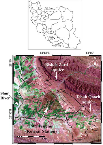
This paper presents results from the BZ aquifer. The thickness of the alluvial fan varies from practically zero on the eastern margin (connection line with mountain) to 43 m, 4 km downstream from the gorge of the BZ watershed, which supplies most of the floodwater to the FWS system. Depth to GW ranges from 4 m in the east to 36 m in the west. The study area is a dry region, with mean annual precipitation of 211 mm, which shows high inter-annual variability. Rainfall mainly occurs from December to March, with a few exceptional events in summer (June–July). The absolute maximum temperature recorded (40–46°C) occurs in July–August and the corresponding minimum (−6 to −1°C) in January–February. Average annual class-A pan evaporation is recorded as 2555 mm.

1.2 Floodwater spreading systems at the Kowsar Station

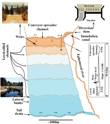
The Kowsar Station was established in 1983 with the aim of desertification control through FWS (Kowsar 1991). FWS systems were planned following the method pioneered by Phillips (1957), improved by Newman (1963) and Quilty (1972), and modified by Kowsar (1991). Eight FWS systems with an extent of 1236 ha were constructed during the 1983–1985 period. Expansion of the FWS systems to 2033 ha was performed from 1996 to 2003. However, the FWS systems are not all covered with floodwater in all of the events; at least one event occurs in non-drought periods that results in full coverage of the systems. Our experience shows that flooding events with flow rate higher than 100 m³ s⁻¹ in Bisheh Zard River cause complete coverage of the systems. Figure 2 illustrates a typical FWS system and its essential components. Details on how FWS systems work can be found in Kowsar (1991, 1995) and Pakparvar (2015).

Figure 2. Generalized diagram of a typical floodwater spreading system. The scales are approximate.

2 Materials and methods

2.1 Water table level and weather data

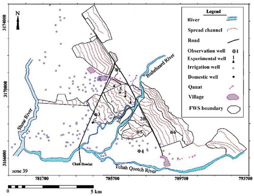
Installation of observation wells (OW) in the study area started in 1992: OW1 and OW4 are located outside of the FWS systems; OW2, OW5 and OW6 are situated inside, with OW5 and OW6 installed in 2005; and OW3 is immediately downstream of the FWS systems (Fig. 3). None of the OWs are located within 200 m of operational wells, so there was no effect on lateral inflow and outflow to the OW from the active pumping zones of adjacent wells. The criterion of 200 m distance is observed (Water Resources Research Organization) in Iran as a guideline for OW installation.

Figure 3. Detailed map of floodwater spreading (FWS) systems, observation wells (OW), experimental wells and distribution of some of the important operational wells in the Gareh Bygone Plain. Observation wells (OW) 2, 4, 5 and 6 are located inside and the others are outside the FWS systems.

Observation well data include the height of the measuring point (MP) above mean sea level, and the depth of the GW relative to the MP. The depth to GW was measured on a monthly basis from 1993 to 2012 by the Fars Regional Water Organization (FRWO). This was performed using an ordinary water level meter with light indicator, with a resolution of 0.01 m. Missing values of water level in the OWs were estimated by employing regression equations between the water levels of the adjacent OWs.

Weather data were available from the Gareh Bygone weather station for 1996–2012. Rainfall data for 1992–1996 were collected from the nearest climatological station (Baba Arab), 15.75 km from Kowsar Station.

2.2 Runon and runoff data

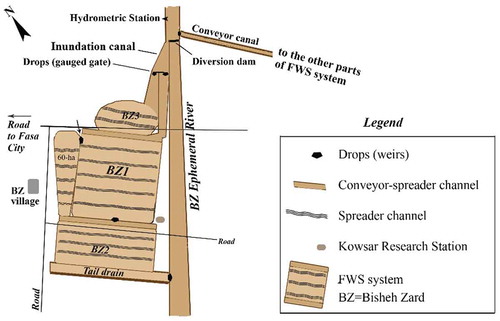
The volume of floodwater diverted to the FWS systems from January 1983 to November 2002 has been estimated and reported (Kowsar Station internal technical reports). Due to lack of data and necessary instrumentation to measure peak flow rates before 2002, peak flow rates for this period have been calculated using an empirical slope–area method as discussed in the following section. Since November 2002, there have been two types of flow measurements in the FWS systems in the study area. First, peak flow was recorded at the hydrometric station, and second, diverted flow inside the FWS systems was measured by broad-crested weirs. In order to explain how the flow measurement was performed in our study site, an example of BZ₁ and BZ₃ FWS systems is given in the following. As depicted in Figure 4, a standard hydrometric station is located upstream of the diversion dam in the BZ ephemeral river. The dam diverts nearly one-sixth of the flow to the diversion canal. The diverted flow, in turn, is divided into two parts by two drops (gauged gates). The wider drop directs the flow to the first (conveyor–spreader) channel of BZ₁ through a conveyor canal. The narrower drop conveys the flow to BZ₃ FWS systems. Surplus flow from BZ₃ joins BZ₁ through three weirs installed on its upslope bank. The flow rate and duration of floodwater diverted into BZ₁ and BZ₃ is measured. There are two other weirs, one installed at the left corner of the first basin and one at the lower end of the sixth basin of BZ₁, which deliver the surplus flow to BZ₂ FWS systems (Fig. 4). The excess flow from BZ₂, which is returned to the main river through a tail drain, is eventually measured in a weir installed at its junction with the river. All of the weirs are constructed on a broad-crested weir design. Thus, the flow that exits through the outlets is also measured, and consequently the volume of floodwater that is harvested by the three systems (BZ₁ to BZ₃) is determined for all events. The flow measurement as explained for BZ₁ to BZ₃ as part of the FWS systems is a good representative of all systems. The flow rate of water entering and leaving the FWS systems in the study area is measured similarly. Therefore, the volume of water that is retained in the individual FWS systems and in the entire project is calculated in every event. To avoid excessive detail, the other parts of the FWS systems are not explained here.

Figure 4. Schematic map of BZ_1, BZ₂ and BZ₃ floodwater spreading (FWS) systems and location of gauged gates for flow measurements. Dimensions are not to scale.

The data needed for flow rate calculations are measured by educated and practically trained technicians and published as technical reports of the Kowsar Station.

2.3 Flow calculations

From 1983 to 2002 the maximum upstream flow rate of the ephemeral rivers was calculated using the slope–area method. The continuity equation, the most basic formula for water flow (Israelsen and Hansen 1965), can be applied in estimating the maximum discharge of an ephemeral river:

(1)

where Q is maximum discharge (m³ s⁻¹), A is flow cross-sectional area at maximum discharge (m²) and V is flow velocity at the highest peak (m s⁻¹). Velocity was estimated using Manning’s equation. This formula can be applied when the channel slope is less than 10% (Linsley et al. 1975) and for conditions of uniform flow in which the water surface profile and energy gradient are parallel to the streambed, and the area, hydraulic radius and depth remain constant throughout the reach (Dalrymple and Benson 1968). These assumptions were met during the flooding events in the two ephemeral rivers (Bisheh Zard and Tchah Qootch), which permits the use of Manning’s equation to calculate flow velocity.

Since 2002 the upstream flow level of the rivers has been continuously determined using data recorded by a lymnograph at a hydrometric station and a rating curve is available for the river section. The observed mean upstream flow with river cross-section profiles was used to determine the cross-sectional area, the wetted perimeter of the flow, as well as the top and bottom widths of the flow area located 5 m upstream and downstream of the lymnograph. The flow rate for broad-crested weirs inside the FWS systems was calculated based on Sargison and Percy (2009).

2.4 Uncertainty of the collected data

The reliability of the collected data was examined prior to their use. The simultaneously recorded rainfall data were used to check the consistency of, and agreement between, measured flows in comparison with the amount of recorded floodwater. In addition, a comparison was made between archived hand-written notes and the published technical reports to remove human error in data transfer. The actual evapotranspiration (ET_a) data, by which the recharge was assessed, had been evaluated by means of cross-validation (Pakparvar et al. 2014).

The long-term measured dataset of GW level was assessed by checking the temporal distribution, its response to the flooding and rainfall events, and a statistical method of empirical quantile–quantile (q-q) plots. A quantile is similar in concept to a percentile; however, a percentile represents a percentage whereas a quantile represents a fraction. If X is the P/100 quantile of the data, then the fraction P/100 of the data values lie at or below X and the fraction (1 – P)/100 of the data values lie at or above X.

A q-q plot for two datasets with respective quantile functions q1 and q2 is a plot of ordered pairs (q1(p), q2(p)) for appropriate values of p. When two datasets of size n are involved, the values of p used to make the plot will be for i = 1, 2, …, n. When two datasets of unequal size are involved, the values of p used to make the plot will similarly be for i = 1, 2, .., n, but here n is the size of the smaller set (Popham and Sirotnik 1992). The quantiles of the sorted values of measured water level data for the OWs were calculated in an Excel spreadsheet and then the quantiles were plotted for every two pairs of the OWs.

2.5 Long-term effect of FWS on recharge

To investigate the role of FWS systems as a potential source of recharge, changes in water level in wells within and outside of the FWS systems were compared for each of the flooding events. A comparison was made between the water level before the occurrence of each particular flood and that measured successively for 4 months after the flooding event. The period of 4 months was selected to cover the maximum change in GW level as influenced by the flooding event. The dataset shows that in most cases the increase in water level continues until the third month and sometimes the fourth month after the flood. To discard the effect of abstractions on changes in water level, data collected for the months of minimum water withdrawal (October–February) were used. The above analysis was carried out for all flooding events during the study period 1993–2012. Of particular importance with regard to these analyses is the case of two consecutive major floods which occurred in 2003/04 and 2004/05. In the first event in December 2003 to January 2004, the FWS systems did not function due to a major repair and maintenance programme, which deprived the aquifer of the generous floods from that event. In the subsequent event in December 2004 to January 2005, the FWS systems were operating properly. This provided a unique opportunity to compare the effect of the FWS systems on aquifer recharge.

Infiltrating rainfall or flooding is not the only cause of changes in water table level. Water table fluctuations are also due to other factors: ocean tides; Earth tides (caused by the forces exerted on the Earth’s surface by the Moon and the Sun); barometric pressure changes; increases in gas pressure in the unsaturated zone; pumping; and lateral flow. These effects need to be avoided, minimized or removed from the water level signals (Crosbie et al. 2005). Unconfined aquifers such as the BZ aquifer here are commonly insensitive to changes in barometric pressure. The effect of ocean tides is not applicable here as the study area is an inland location. Lateral flow is insignificant as the wells are located in a relatively flat plain with low hydraulic gradient. Pumping by production wells is a major cause of falls in water level after recharge events and must be taken in to account in all of the analyses in the study area.

A hydrograph of GW in the study area was plotted based on the mean GW level for each month and employing the grid layers generated by Surfer software (Surfer 13, ®Golden Software, LLC). Rainfall depth and simultaneous mean GW level of the study area were also plotted concurrently to inspect the effect of drought on the hydrographs.

2.6 Quantification of recharge

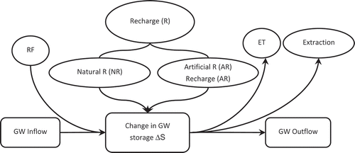
The method employed here is based on the premise that a rise in GW level in unconfined aquifers is due to recharge water arriving at the water table. Change in GW storage is calculated as:

(2)

where ∆S is change in GW storage, S_y is specific yield, h is water table height, and t is time (Scanlon et al. 2002). Equation (2) assumes that water arriving at the water table goes immediately into storage and that all other components in the GW budget, including ET and inflow and outflow from the water table, are zero (Healy and Cook 2002). This occurs in practice during the period of recharge. Therefore, equation (2) is applicable for a short time when the magnitude of recharge is high, the vertical flow is significant in comparison with the lateral underground flow, and for each individual water table rise. For long-term determination of recharge (e.g. a hydrological year), the long-term change in GW budget components must be considered when using WTF methods (Healy and Cook 2002). A general budget equation for the saturated zone modified based on Hoque et al. (2007) can be written as:

(3)

where E is extraction from the aquifer, ∆S is change in GW storage (or change in saturated pore volume), R is recharge of GW, RF is agricultural return flow, and are subsurface flow on and off, respectively, and ET^gw is ET from the GW table, all on a volume basis. The ET^gw may be neglected as direct ET from deep water tables in arid regions is insignificant, unless deep plant roots take up water from the water table. Similarly to the short-term assumption in equation (2), the components of subsurface flow and may be neglected in the long term as well, because of the balance between the lateral input and output of water in the aquifer. Recharge can be natural or artificial. Natural recharge pertains to diffusion from upland and adjacent aquifers and water infiltration in river beds, whilst artificial recharge is that influenced by an engineered structure to generate or intensify the recharge of GW. With ∆S calculated from the WTF (equation (2)), recharge can then be determined as the remainder of equation (3). The saturated zone water budget components are illustrated in Figure 5.

Figure 5. Schematic of water budget for the saturated zone. Extraction is any type of direct withdrawal of groundwater, e.g. pumping; ET is evapotranspiration and RF is agricultural return flow.

The method used by Hoque et al. (2007) was applied here for estimating recharge for the hydrological year 2010/11 when all the necessary input data were available. Equation (3) was solved to find the recharge (R) when the other components such as extraction from the aquifer (E), change in GW storage (∆S) and return flow (RF) were known:

(4)

The ET from the GW (ET^gw) was considered to be the water consumed by tree plantations, which have access to GW by their deep tree roots. The subtraction of inflow and outflow to the GW () in equation (‎3) was assumed to be zero in a hydrological year. Thereafter, the artificial recharge (AR) was calculated (as explained in Section 2.7). As a result, the contribution of AR to total recharge (R) was determined. The remainder after subtraction of AR from R was ascribed to natural recharge (NR). The determination of different sources of NR (river bed infiltration, rainfall infiltration in the uplands, diffusion from the adjacent aquifers, etc.) and its quantification is beyond the objectives of this study, so is left to be studied in future research.

2.6.1 Amount of extraction from the aquifer

Extraction from the aquifer was estimated using two different methods. First, the annual volume of water withdrawal from the BZ aquifer measured by Hosseinimarandi et al. (2011) through a field survey was used. The survey results include the location of irrigation wells, their discharge rate, the daily hours of operation and the number of operation days per year. The field data recorded by Hosseinimarandi et al. (2011) were used to check and recalculate the flow discharge. In addition, the results of a survey conducted by FRWO (see Section 2.3) containing the total number of pumping wells installed in the study area, the installation year, the depth of the wells and, in some cases, the pumping rates were used to cross-check the data. These two sets of data were compared and checked in order to minimize errors in the well locations and discharge rates. Those wells located inside and near the BZ aquifer were removed from the whole dataset. The total extraction by water withdrawal was calculated for each well’s discharge and working hours and summed for the all wells.

Second, the volume of applied irrigation water was measured in 12 wheat and 10 forage corn irrigated fields in the area during the growing season of the hydrological year 2010/11. To do so, well discharge was measured in the head ditch above each field using a cut-throat flume (Walker 1989). This was then converted to seasonal volume of applied water per hectare using the time of application for each turn and the number of irrigations during the season. The total volume of applied water for the cultivated farm fields was then calculated using the measured area provided by remote sensing (Pakparvar et al. 2014).

2.6.2 Change in GW storage (saturated pore volume)

The WTF method was used to calculate the change in GW storage. The depleted volume was calculated by employing the volume calculation facility of Surfer software. This finds the volume between the two surfaces given as grid files. As described by Hoque et al. (2007), the volume is defined by a double integral:

(5)

Surfer computes this by first integrating over x (the columns) to obtain the areas under the individual rows, and then integrating over y (the rows) to get the final volume.

The depths to the impermeable layer in lithological logs of the six OWs and those reported by Hosseinimarandi et al. (2011) for irrigation wells were used as the lower boundary of the aquifer. The GW levels in 1993, 1997, 2003, 2005 and 2012 were considered as the upper boundary. Dewatering volume was calculated by subtracting aquifer volume for each year from its previous one. Selection of the above-mentioned years was based on significant changes in the hydrograph slope in those years.

Saturated pore volume was calculated as the product of specific yield (S_y) and dewatered volume of the aquifer. Values of specific yield reported for the BZ aquifer are 0.05 (averaged) by Hashemi et al. (2013) and 0.008 by Hosseinimarandi et al. (2011) employing the pumping test. Values as low as 0.008 were obtained in some of the measurements performed in the above two studies. The underestimation of S_y by the pump test has been experienced by other authors (Nwankwor et al. 1984, Moench 1994). Crosbie et al. (2005) showed two to three times underestimation of S_y by the pump test as evaluated by a mass balance study using chlorine. Therefore, the method used in this study is based on the physical concept of water retention in porous media using a soil moisture retention curve (Crosbie et al. 2005):

(6)

where θ_s is the saturated soil-water content and θ_r, the residual water content, is defined as the water content for which the gradient (dθ/dh) becomes zero (excluding the region near zero matric potential, which also has a zero gradient). However, since specific yield is water content of the porous media that can be easily drained, moved and pumped out, the lower boundary of water content was set to the field capacity (FC), which was considered as a soil-water potential head of −330 cm (Brady and Weil 1996, Kolay 2008) The term θ_r in equation (6) was therefore changed to θ_FC. The amount of soil-water content assigned to FC depends on soil hydraulic properties, especially the pore size distribution. As the soil-water potential in which the water is retained by the soil particles can better explain this term, the FC has been defined as soil water corresponding to a particular soil-water potential and normally considered as −1/3 atmosphere or −330 cm.

Three experimental wells (28 to 32 m in depth) were dug in this study from May to September 2008 and were explored to determine the depth and distribution of the layers (Fig. 3). Seven representative layers (RL) were recognized, and these were repeated throughout the experimental well profiles. Soil samples were taken from the seven RLs of these experimental wells and physical properties including texture, fraction of stones and water content were measured. Complete water retention curves including water content at saturation and −330 cm were established for the <2 mm fraction using a sand box apparatus and pressure plate (Table 1). Due to the presence of stone fractions, water contents were adjusted using the Bouwer and Rice (1984) equation:

(7)

where θ_b is the water content of bulk material (undisturbed fine soil plus stones), V_r is the volume fraction of stones, and θ_f is the water content of the fine soil. The calculated specific yields of the RLs were then used to assign a value to the aquifer S_y. To do this, a weighted average S_y was calculated for the entire well profile considering the occurrence of each RL throughout the profile by multiplying each layer thickness by its pre-defined S_y value, and then summing up the products and dividing by the depth of all the summed-up layers. The two surface layers were excluded from the weighted average computation because of their absence in sub-surface layers.

Table 1. Retention curve data and input parameters for S_y calculation.

Layer	Stoniness	Depth (m)	Potential (cm)				Sy
			0		−330
			θv (m^3 m^−3)
			m	c	m	c
A	0.07	0–0.1	0.45	0.42	0.20	0.19	0.23
B	0.22	0.1–0.42	0.44	0.34	0.07	0.05	0.29
C	0.54	0.42–1.0	0.38	0.17	0.18	0.08	0.09
D	0.66	1.0–1.3	0.35	0.12	0.05	0.02	0.10
E	0.07	1.3–1.8	0.39	0.36	0.08	0.07	0.29
F	0.53	1.8–2.25	0.38	0.18	0.05	0.02	0.16
G	0.11	2.25–3.35	0.4	0.36	0.08	0.07	0.29

These representative layers are repeated along the aquifer profile in 30 m deep experimental wells, except for A and B. θ_v: volumetric soil-water content; m: measured θ_v; c: corrected θ_v based on the stoniness (using equation (‎27)); S_y: specific yield calculated as the difference between θ_v of the saturated soil and the field capacity (potentials of 0 and 330 cm, respectively). The value of S_y for the entire aquifer was obtained as 0.18 based on a weighted average of the aquifer layers.

2.6.3 Agricultural return flow and ET from the GW

Return flow was calculated as 22.5% for the same study area by Pakparvar et al. (2014). The component of applied water consumed by crops and tree plantations was determined by ET_a mapping using the SEBS (surface energy balance system) model and 32 successive Landsat images. Parameterization of SEBS was primarily optimized by assessing against observed ET data and then used for calculating the yearly ET_a. According to the availability of Landsat images at the time of study, the ET_a calculation was made for the period from October 2009 to December 2010. Since the cropped area in the two successive hydrological years 2009/10 and 2010/11 was practically the same, the return flow used was for the hydrological year 2010/11 for which the full input data of the water budget were available. In the same way, the ET^gw component was calculated based on the summed annual ET_a data from the ET maps and the area of tree plantations.

2.7 Quantification of artificial recharge

The contribution of the FWS systems to total recharge was assessed using the following methods in order to cross-check the results.

2.7.1 Application of flow data

The component of water in a recharge pound consumed by total losses (open water evaporation plus ET), when subtracted from the amount of pounded water, is net total infiltration (Hendrickx et al. 1991). Because of the deep GW table and due to the coarse-textured stony soils in the vadose zone, the positive flux (towards the soil surface) resulting from capillary movement after the event was assumed negligible. Therefore, the net infiltration to the deep layers was counted as the net recharge and the net recharge was considered as artificial recharge based on the flooding data inside the FWS systems. Indeed, the lateral movement would cause some of the infiltrated water to move to the natural drainage (the Shour River) but the proportion of vertical to lateral movement is not large enough to substantiate the lateral movement. To justify this, it should be noted that the horizontal hydraulic conductivity of aquifers similar to the one in our study (medium to coarse gravelly material) has been reported as 0.02–1.02 cm d⁻¹ (Domenico and Schwartz 1990), whereas the vertical hydraulic conductivity measured by Pakparvar (2015) varied between 17 and 2840 cm d⁻¹, which is far higher than the expected horizontal hydraulic conductivity. Therefore, the assumption of neglecting lateral movement, at least when vertical infiltration due to a flooding event is in progress, is reasonable.

Evaporation occurs over a long period until all of the ponded water is infiltrated. Therefore, the evaporation losses during a given period depend on the duration of infiltration and on the infiltration rate. To evaluate the recharge, the equation derived by Hendrickx et al. (1991) was used:

(8)

in which AR is the net artificial recharge (mm), D is the depth of water applied for recharge (mm), i is the infiltration rate (mm d⁻¹), e is the open water evaporation during the period of infiltration (mm d⁻¹), and ∑ET is the cumulative ET after all water has infiltrated (mm). The infiltration rate values for surface soils in the FWS systems of the study area, measured at several points by Rahbar et al. (2016), were used to prepare an infiltration map using Surfer software. Normally the floodwater retained within the FWS systems infiltrates in less than 48 hours. The FWS systems dry out in summer after 10–15 days and in winter after 30–40 days. Open water evaporation for a duration of 6 days of the events was taken from weather data. The cumulative ET was calculated based on ET maps as described by Pakparvar et al. (2014). As some of the infiltrated water is lost by ET, the time after flooding events when ET is taking place was considered as 30 days based on observations of soil-water content at different depths by Pakparvar (2015). Long-term data show that soil-water content of the topsoils (to a depth of 60 cm) resumes its initial level before a rainfall or a flooding event in a maximum of 1 month.

2.7.2 Water budget method

Recharge (determined in Section 2.6) is based on the water budget of the whole Bisheh Zard aquifer for the entire hydrological year (2010/11) and is therefore considered as total recharge. In order to quantify artificial recharge, the water budget equation (equation (‎3)) was employed again, but the time span was limited to the flooding period in the area that is under the immediate influence of FWS systems. This area was delineated by constructing polygons surrounding the FWS systems including the location of the six OWs. Then the water level before the occurrence of each particular flood was compared with the maximum water level measured after the flooding event. These two sets of GW level data for the OWs were used to construct piezometric maps using Surfer software. The areas outside the boundary of the FWS systems were excluded using the Blank module in Surfer. Then the above-mentioned piezometric maps were introduced to Surfer’s Volume module as the top and the bottom layers, respectively, to calculate the volume of the aquifer in which recharged water was stored. The resulting volume was then multiplied by S_y to obtain the change in GW storage (∆S) in the water budget equation.

The E component is considered to be equal to agricultural water extraction for the same time period as for the ∆S calculation and for the farmlands located inside the pre-defined boundary of the FWS systems. To calculate E, the amount of applied water to the cultivated (not fallow) part of the farmlands inside the FWS systems boundary was calculated based on the measured applied water per hectare multiplied by the total area. The RF component was then calculated by subtracting E from total ET of the corresponding farmlands. Total ET, in turn, was calculated by summing up the ET values extracted from ET maps generated by remote sensing (Pakparvar et al. 2014). The ET^gw component was calculated based on the summed annual ET_a data from the ET maps and the area of tree plantations.

3 Results and discussion

3.1 Water level data quality

As inferred from the empirical q-q plots (Fig. 6), the tendency of scatter points to the trend line is different for the OWs; meaningful correlation in q-q plot is seen in all of the OWs, at least for one adjacent OW.

Figure 6. Empirical q-q plots for the water level data of the observation wells (OW) 1 to 6.

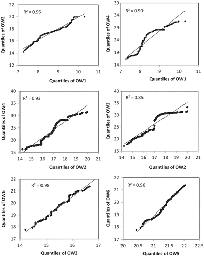
When a q-q plot is reasonably linear, one may conclude that the two distributions involved have similar shapes. When there are marked departures from linearity, the character of those departures can reveal the ways in which the shapes differ (EPA 2000). When several datasets with similar temporal measurement intervals show linearity in cross-validation using empirical q-q plots, this is adequate evidence of reliability of the measurements (Popham and Sirotnik 1992). Therefore, it can be concluded that the reliability of the water level measurements is similar for the OWs of interest in this study.

3.2 Spatial and temporal changes in water level

Figure 7(a) depicts the synchronized rainfall and GW hydrograph for the study area. The generalized hydrograph shows an increase in water level from 1993 to 1997, a steep decrease from 1997 to 2004, and a gradual decrease from 2005 to 2012. The difference between the initial and final GW levels is about 6 m. The annual trend of rainfall during the study period revealed some irregularity, though a general declining trend can be perceived.

Figure 7. (a) Temporal trend of rainfall and groundwater hydrograph. (b) Temporal trend in the number of wells in the region. GBP is the whole Gareh Bygone Plain and BZ is Bisheh Zard aquifer. WL is groundwater level height.

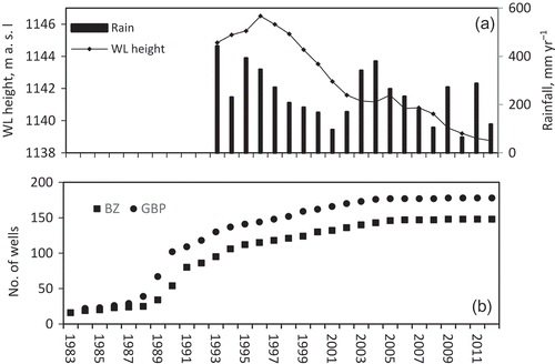
As inferred from Figure 7(b), the number of irrigation wells started to increase from the beginning of construction of the FWS systems in 1983, but an expedited increase is shown from 1989 to 1994 (72 wells in 5 years). The number of wells continued to increase until 2005, after which it remained stable up to 2012. The recession trend in GW from 1997 to 2004 coincided with recurrent droughts and the increase in the number of irrigation wells. The increase in the amount of annual rainfall from 2000 to 2005 slowed down the rate of decrease in water level. The recent drought from 2005 to 2012 increased the rate of drop in water level again.

To quantify the influence of rainfall and number of dug wells on the GW level change, a multiple linear regression was made between the annual rainfall and number of dug wells in Bisheh Zard aquifer as independent variables and the mean GW level as a dependent variable (Table 2). The model itself has an F value of <0.001 and an adjusted R² of 0.79, which is significant at the <0.01 level of confidence. Incorporation of the independent variable “number of wells”, which has a low p-value (here, p < 0.01), is likely to be a meaningful addition to the model because changes in the predictor’s value are related to changes in the dependent variable. Conversely, a larger insignificant p-value (here, p = 0.81) of the “rainfall” variable suggests that changes in this variable are not associated with changes in the response.

Table 2. Influence of the rainfall and number of dug wells on the GW level as indicated by multiple linear regression.

Summary of the model
R^2	0.81
Adj. R^2	0.79
Observations	20
ANOVA
	DF	SS	MS	F	Sig. F
Regression	2	101.94	50.97	36.27	7.36E-07
Residual	17	23.89	1.41
Total	19	125.83
Variables
	Coeff.	SE	t Stat	P-value
Intercept	1161.38	2.87	404.23	2.67E-35
No. of wells BZ	−0.1419	0.0186	−7.62	7.01E-07
Rain	−0.0007	0.0029	−0.24	0.81

Multiple linear regression between the GW level as dependent (Y) and the number of dug wells in Bisheh Zard aquifer (Wells BZ) and annual rainfall (Rain) as independent (X1 and X2) variables. Adj.: adjusted; ANOVA: analysis of variances; DF: degree of freedom; SS: sum of squares; MS: mean of squares; Sig.: significance.

Although some studies have shown high correlation between water table fluctuation and precipitation (Crosbie et al. 2005, Rimon et al. 2007, Yu and Chu 2012), a statistically significant correlation could not be established between the two sets of data. Therefore, the decreasing trend in GW level cannot be statistically ascribed to the temporal trend of rainfall. However, the timely influence of rainy years on the GW hydrograph can be implied. For instance, the increase in GW level during the period 1993–1997 was concurrent with large storms in 1993 and 1996. A drought period from 1997 to 2000 coincided with severe recession in the GW level.

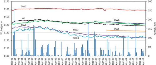
To demonstrate the role of the FWS systems in the above setting, the behaviour of individual wells located inside and outside the FWS systems was examined. Water level change showed no trend in OW1 (Fig. 8). This could be due to the location of the well, which is close to a fault supplying water to the plain (Hashemi et al. 2013). Observation wells OW2, OW3 and OW4 revealed the same temporal trend as the general hydrograph of the study area. However, OW2, being located inside the FWS systems, showed a greater resistance to the drought periods and extractions than OW3 and OW4. The drop in the water level in OW2 in the period 1997–2004 was 2.07 m, while OW3 and OW4 showed drops of 9.0 and 11.26 m, respectively, in the same period. This clearly demonstrates the impact of the FWS systems on the recharge of GW. It can also be concluded that OW3 and OW4 are located in the vicinity of the pumping wells (or extensive farming area), where abstraction has a substantial effect on GWL drawdown relative to the area around OW2.

Figure 8. Changes in groundwater level (WL) height in the observation wells (OW). OW5 and OW6 were installed in 2005. The line “All” represents the generalized hygrograph of the Gareh Bygone Plain.

As shown in Table 3, an anomaly was observed in the amount of rainfall and the volume of flood, in that the extent of rainfall and its subsequent flooding are not always proportional (some higher rainfall resulted in lower volume of flooding). The reason for this diversity is the disparity in the location of rainfall. When the rainfall covered both the highland basins as well as the Gareh Bygone Plain, maximum runoff occurred and the volume of the resulting flood flow was relatively high. In contrast, when the rainfall was limited to within the plain, the resulting flow in the ephemeral rivers was not enough to produce extreme flooding. The season of flood occurrence is the other source of variation. In summer time, when the soil surface is barren due to drought, runoff is much higher than in the winter. In spite of the low rainfall during this period, numerous flooding events occurred and the FWS systems were operating (Table 3).

Table 3. Important flooding events recorded at Gareh Bygone Plain.

Date of flooding	Flood (hm^3)^(a)	Rain (mm)	Date of flooding	Flood (hm^3)^(a)	Rain (mm)
08.02.93	NR	NR	6–7.12.03	3.14	66.0
27.03.94	NR	25.0	27.01.04	13.58	225.5
03.12.94	NR	31.0	15.12.04	22.17	242.5
08.03.95	NR	1.5	20–23.01.05	8.38	211.0
24.07.95	NR	30.0	30.03.06	22.20	150.0
06.12.95	NR	49.0	5.09.06	8.38	61.5
25.03.97	NR	35.0	4.02.07	0.16	28.0
02.01.98	NR	27.0	24.07.07	0.18	11.5
02.03.99	NR	118.0	9.09.08	1.26	91.0
08.07.99	NR	6.0	30.03.09	0.24	23.5
16.12.01	NR	21.0	8.12.09	0.19	18.0
12.01.02	NR	47.0	5–27.02.10	2.43	54.5
22.12.02	0.50	33.0	31.1–2.2.11	6.92	149.0
23–26.03.03	3.60	21.0	23.11.11	0.84	20.5
16.08.03	0.40	36.0	26.02.12	1.65	23.2

^(a) The volume of retained flow in the system (diverted inflow minus outflow) in hm³ (i.e. million m³). NR: not recorded.

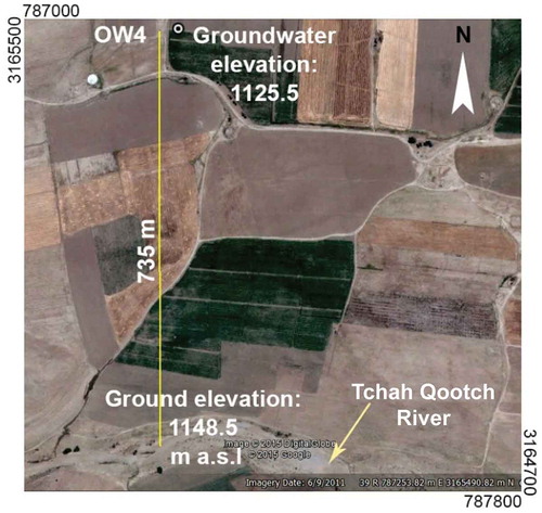
During the period 2005–2012, the hydrographs of the three wells (OW2, OW3 and OW4) showed a similar mild drop. During this period, the number of floods had decreased due to recent drought and therefore the role of the FWS systems diminished. Hence, the observation wells were expected to show similar behaviour. In this period, a greater decline in GW level relative to the previous period (1997–2004) was expected. The higher drop in the 1997–2004 period is related to a sudden increase in the number of wells (Fig. 8). The drops in the above-mentioned OWs were 2.9, 3.4 and 0.7 m, respectively. The lower drop in OW4 could be due to recharge from the Tchah Qootch River located south of OW4 (Fig. 9) as a supplemental source of recharge. The GW flow direction from the river towards the OW4 was obvious in the piezometric maps (not shown here). This fact is evident by comparing the elevation of the Tchah Qootch River bed at the closest location to the GW level of the OW4 (1145.5 m a.s.l.), which is higher than the GW elevation of this OW (1125.5 m a.s.l.) (Fig. 9). Eight years (2005–2012) of data collection for the other two OWs show recessions of 1.4 and 3.2 m for OW5 and OW6, respectively. Thus, OW5 and OW6 show the same trend as OW2 and OW3.

Figure 9. Location of observation well 4 (OW4) in relation to the Tchah Qootch River and the proportional ground and groundwater elevations. The image is taken from GoogleEarth^TM of 6 September 2011. The corresponding groundwater level of OW4 is taken from the data of the same month in 2011.

3.3 Substantiating the effect of the FWS systems

Some selected data for flood occurrence and the corresponding values of the rainfall are shown in Table 3. Rainfall data were accessible from 1993 and floodwater diversion data have been collected since December 2002.

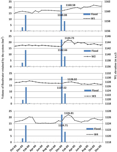
To demonstrate the effect of the FWS systems on aquifer recharge, the behaviour of OWs 1, 2, 3 and 4 is examined more closely in response to the flooding events (Fig. 10). In the year 2003 the FWS systems were not functioning due to a necessary repair and they were re-started in 2004. The hydrograph of OW2 shows that the response to a 22.17 hm³ of flood in 2004/05 resulted in a considerable rise (2.05 m) after 2 months. The change in water table level due to the previous flood of 13.58 hm³ in 2003/04 was measured as 0.50 m. Although the magnitude of the flood in 2004/05 was higher than the previous year, OWs outside the FWS systems (OW1, OW3 and OW4) showed similar responses to both flooding events, and therefore the flooding magnitude may not be the reason for the sudden change in OW2 in the latter year. The change in water level in OW2 showed a common trend in 2003/04, which was due to natural recharge (river bed and other sources), whereas in 2004/05, the sudden rise in water level was the direct response of the operation of FWS systems. The other wells located in the vicinity of the FWS systems (OW3 and OW4) exhibited different behaviour from OW2. In 2003/04, when the FWS systems were not functioning, OW3 showed a 0.3 m rise, similar to that of OW2; however, in the following flood in 2004/05 when the FWS systems were functioning, the rise in water level of OW3 (0.5 m) after 3 months was much less than that of OW2 (2.05 m). The sustained floodwater on the FWS systems was the same in both of the events because they occurred in the same season for the two years (December and January). This difference is expected to occur for two reasons. First, due to the location of OW3, which is outside the FWS systems, a delay in reaching the peak in water level as compared to OW2 is anticipated; and second, due to being in the vicinity of the farming wells, the water level did not rise in the following months.

Figure 10. Response of water table to flooding events. The FWS systems were not functioning during the first event of December 2003 to January 2004, but were functioning during the second event of December 2004 to January 2005. WL: groundwater level (hm³ is million m³).

As described by Bouwer (2002), if no clogging layer exists at the bottom of an infiltration basin and the basin is “clean”, the water table rises to the water level in the basin, and the water in the basin and in the aquifer are then in direct hydraulic connection. In this case, a mound underneath the infiltration basin is expected, as evidenced by the OW2 data for 2004/05. Therefore, this proves the hydraulic connection between the FWS systems and the aquifer, and infers an adequate infiltration rate for its surface after a long period (32 years) of functioning.

The rise in the water level in OW4 (1.20 m) was much more noticeable than that at OW2 and OW3 in the first flood event. This supports the claim mentioned above that there was some recharge from the Tchah Qootch River during the flooding events. A comparable rise to that of OW2 was seen in the subsequent flood (1.90 m).

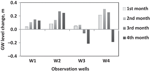
In addition to the above analysis on two successive floods, long-term comparison was made between wells in response to all of the flooding events. The mean difference between water level in the wells before the flooding events and the corresponding values for 4 months after the events is depicted in Figure 11. As expected, OW2 shows a positive change up to 4 months after the storms. This is true for OW1 as well, but to a lesser extent. OW3 shows the lowest rise in water level compared to the other wells. OW4, located outside the FWS systems, shows the highest rise in water level up to the third month after the events. It is seen that the long-term behaviour of wells supports the determinant role of the FWS systems in aquifer recharge.

Figure 11. Variation in average groundwater (GW) level in the observation wells before and after flooding for four consecutive months during the period of minimum water withdrawal. 1st to 4th month refer to water level changes in the months after the flooding events.

3.4 Dewatering of the aquifer

The data from which S_y was calculated are presented in Table 1. The mean S_y, calculated for the entire aquifer layer, was 0.18. The specific yields, as reported by several authors in lithological materials similar to those in our study area are 0.18–0.36 (Crosbie et al. 2005), 0.063 (Moon et al. 2004), 0.2–0.25 (Gutentag et al. 1984), and 0.15 (Hoque et al. 2007). In addition, as indicated by Bouwer (2002), the fillable porosity to be used in the equations for mound rise is usually larger than the specific yield of the aquifer, because vadose zones are often relatively dry, especially in dry climates and if they consist of coarse materials such as sands and gravels. The fillable porosity should be taken as the difference between the existing and saturated water contents of the material outside the wetted zone below the infiltration system. Therefore, according to the literature, the value of S_y determined in this study as 0.18 is justified, and was chosen as the multiplier to convert the dewatered volume to the dewatered pore volume. The piezometric maps employed to calculate the amount of change in water storage of the two successive years of the 1992 and 1993 are presented in Figure 12. The same procedure was followed to compute change in water storage for 1992 to 2012. An estimate of the change in storage volume in this period is presented in Figure 13.

Figure 12. Three-dimensional representation of the two overlain groundwater level surfaces—that of 1997 over that of 1993—used to calculate the change in aquifer storage between these two years.

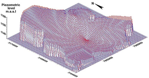
Figure 13. Temporal changes in storage volume of the aquifer.

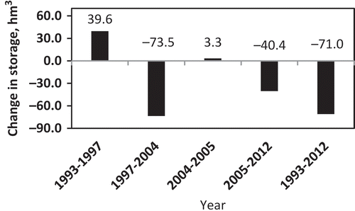
A noticeable positive volume change of 39.6 million m³ (hm³) was observed during 1993–1997, which is approx. 8.0 hm³ per year. The second increase of ~3.3 hm³, although a minor one, occurred during 2004/05. Apart from this, continuous dewatering occurred from 1997 to 2012 with an estimated depletion of 113.9 hm³, giving a net result of 71.0 hm³ of dewatering for the period 1993–2012. This is a stern warning that the limited natural and induced recharge cannot supply unlimited withdrawal; therefore, given the shallow depth of the aquifer, it will probably dry up in the very near future.

3.5 Recharge estimation

Results for extraction from the aquifer are presented in Table 4. Applied agricultural water and withdrawal were estimated as 13.82 and 15.27 hm³, respectively. These two methods of extraction estimation resulted in different but close values. Higher estimation for withdrawal is expected as some of the extracted water is not used for irrigation due to the conveyance losses between the farm fields. The amount of loss is 1.45 hm³ or 9.5% of the withdrawn water. Therefore, extraction volume based on the withdrawal water (15.27 hm³) was chosen as the basis for further calculations.

Table 4. Calculations of water extraction in the hydrological year October 2010 to September 2011.

Based on measured applied water
Consumer	Area(ha)	Ave. applied^(^a^)(m^3 ha^−1)	Consumption(hm^3)
Winter crops	1184	4800	5.68
Summer crops	725	9800	7.11
Tree plantations^(^a^)	132	7450	0.98
Domestic use			0.05
Sum			13.82
Based on water withdrawal
	No. wells		Mean discharge	Mean working time	Abstraction
Source	Total	Active	(L s^−1)	(h year^−1)	(hm^3)
Wells	148	88	7.95	5655	14.24
Tree plantations					0.98
Domestic use					0.05
Sum					15.27
Transport losses (%)					10.30

^(a) Applied water for tree plantations is calculated by ET_a mapping. Water consumption by tree plantations is considered as a source of GW extraction due to access of tree roots to the GW table (observed in this study at the depth of 28 m). The total extraction by water withdrawal was calculated for each well’s discharge and working hours and summed for all the wells. The means are shown here to be indicative of the wells’ discharge and working times. Transport losses are calculated as the ratio irrigation applied/withdrawn water, (5.68 + 7.11)/14.24.

Of the 15.27 hm³ extracted water from the aquifer, 3.2 hm³ was estimated as the irrigation return flow, which was assumed to return to the aquifer. As the extracted water for irrigation was 14.24 hm³ of the 15.27 hm³, the return flow of 3.2 hm³ was 22.5% of the irrigation applied water. This percentage is close to the values reported for the main crops in the dry states of the USA (15–55%; average 24%) (Sabol et al. 1987) and the value of 24% reported by Jafari et al. (2012) for a similar environment and management settings to our study area. There is uncertainty about the specific time when the return flow reaches the GW (Bouwer 1987). However, continuation of farming activities in successive years guarantees a permanent irrigation return volume of what is calculated for a particular year.

The dewatered pore volume of the aquifer was calculated to be 22.95 hm³, and with S_y of 0.18, the depleted water from the aquifer (∆S) was about 4.13 hm³ during the hydrological year 2010/11. The return flow was assumed as 3.2 hm³, hence the recharge was estimated to be 7.94 hm³, which is a consequence of both artificial recharge and natural replenishment (Table 5).

Table 5. Water budget of the total recharge in the hydrological year 2010/11.

Input (hm^3)		Output (hm^3)
∆S	4.13	E	15.27
RF	3.20
R	7.94
Total	15.27		15.27

∆S: change in GW storage; R: recharge; RF: return flow; E: total extraction from the GW. R is calculated as the remainder of the water budget (equation (4)).

3.6 Artificial recharge estimation

3.6.1 Based on the flow data

The artificial recharge data in 2010/11 are presented in Table 6. During the flooding events from 28 January to 2 February 2011, a total volume of 6.92 hm³ of floodwater was retained in the BZ FWS systems. These events ponded the entire FWS systems of 2033 ha (22.33 hm²) and resulted in an average depth of 0.34 m on the FWS surface. The duration of the infiltration was counted as 6 days, evaporation rate (e) as 0.024 m d⁻¹, the sum of ET (∑ET) after the event for the 30 days was calculated as 0.075 m, and the weighted average of infiltration rate (i) as 0.28 m d⁻¹, Therefore, the recharge water was estimated as 0.24 m using equation (8) (Table 7).

Table 6. Flow rates of floods diverted into the FWS systems in 2011.

Flooding date	Mean discharge	Duration	Inflow	Outflow	Retained flow
	(m^3 s^−1)	(h)	(hm^3)	(hm^3)	(hm^3)
28 January 2011	115	3.0	1.24	0.25	0.99
1 February 2011	159	13.0	7.44	4.62	2.82
2 February 2011	203	8.5	6.21	3.10	3.11
Sum			14.90	7.97	6.92

Inflow and outflow are the volume of incoming and outgoing flood flow to the floodwater spreading system. Retained flow is the volume of flood flow retained by the system.

Table 7. Components of the recharge calculation based on the flow data.

Retained flow (hm^3)	Area (ha)	D	e	i	∑ET	AR
						(m)	(hm^3)
6.92	2033	0.34	0.024	0.28	0.075	0.24	4.84

D: depth of ponded water (m); e: evaporation rate (m d⁻¹); i: infiltration rate (m d⁻¹); ∑ET: sum of ET in the 30 days after flooding event (m); AR: recharge.

As a result, the volume of artificial recharge due to the FWS on the 20.33 hm² surface area of the FWS systems was estimated to be 4.84 hm³. The ratio of artificial recharge to the depth of ponded water (0.24 and 0.34, respectively) was 0.7. Hendrickx et al. (1991) reported similar values (0.6 to 0.8) for an alluvial stony fan resembling our study site.

3.6.2 Based on the water budget

The contour lines of change in GW level for the 3 months after the flooding events in the surrounding area of the immediate influence of FWS systems are presented in Figure 14. A mound of GW rise was formed in the southeast part of the FWS systems, showing the area of maximum influence of the system. The rise then gradually decreased in the west and southwest directions. The surroundings have an area of 3232 ha and the volume of GW rise was calculated as 9.03 hm³. According to the previously determined value of S_y (0.18), the change in the volume of storage due to artificial recharge (∆S) was obtained as 1.625 or approx. 1.63 hm³. During the 3 months after the event (the period considered for GW rise), some portion of the recharged water was used for irrigation and consumed by tree plantations (Table 8). The cultivated area of the farmlands located inside the boundary of the FWS systems was measured as 705 ha, the rate of applied irrigation was 4800 m³ha⁻¹; hence, the extracted volume for irrigation purposes was determined to be 3.38 hm³. The amount of water extracted by tree plantations was calculated based on summed ET_a in the same period to be 2300 m³ha⁻¹ or 0.30 hm³ for the total area. The volume of RF was calculated to be 0.73 hm³ (22.5% of the 2.95 hm³ used for irrigation + 0.31 hm³ conveyance losses) and, therefore, the artificial recharge is estimated as 4.46 hm³ (Table 9).

Figure 14. Change in GW level contour lines in the period of 3 months after the flood event of 28 January to 2 February 2011.

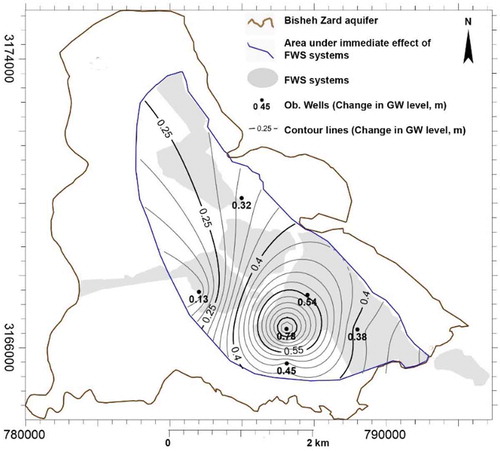
Table 8. Extraction from the aquifer during the period February–April 2011.

Land use	Area (ha)	Extracted water
		(m^3 ha^−1)	(hm^3)
Irrigated crops	615	4800	2.95
Transport losses (10.3%)			0.31
Tree plantations	132	2300	0.30
Total			3.56

The area of irrigated crops is measured for the cultivated parts of farms located in the FWS systems area of influence.

Table 9. Water budget for January–April 2011 for the area under the immediate influence of FWS systems.

Input (hm^3)		Output (hm^3)
AR	4.46	E	3.56
RF	0.73	∆S	1.63
Total	5.19		5.19

∆S: change in GW storage; AR: artificial recharge; RF: return flow; E: total extraction from the aquifer. AR is calculated as the remainder of the water budget equation (equation (4)).

Comparison of the two methods of artificial recharge estimation and their ratio to total recharge is shown in Table 10. The contribution of the artificial recharge is calculated as 4.84 and 4.46 hm³ by the flow data and the water budget, respectively. The lower value obtained by the water budget method is expected as it is essentially based on the change (rise) in GW storage as influenced by the net recharge of the GW, and the one obtained by the flow data is based on the total infiltrated water to the deep layers. Consequently, the difference between the two values appears to be the portion of net infiltration (7% of 4.84 hm³) that did not contribute to recharge and moved horizontally. Conditional to selecting one of the resulting values for the artificial recharge, 56–61% of the total recharge could be attributed to the impact of the FWS systems for that hydrological year. Hashemi et al. (2013) found an average ratio of 61% by a modelling approach in the same study area, with 80% for extreme events and 41% for normal events. As they did not define the criteria for differentiating between extreme and normal events, we cannot judge whether the event in this study is considered as extreme in order to compare it with their results. However, looking at the range of flooding event volumes (Table 3) in the study site, the studied event can hardly be assumed as extreme. The study area received 276 mm of precipitation in the hydrological year 2010/11, so, considering the BZ aquifer’s areal extent as 7600 ha, the equivalent volume of rainfall is 20.9 hm³. The remainder of the total and artificial recharge subtraction is counted as natural recharge, therefore, and the calculated natural recharge is 2.87–3.25 hm³ and the contribution of precipitation to the natural recharge is 14–15%. The magnitude of natural recharge has been studied worldwide by many authors. A review undertaken by Bouwer (2002) revealed that natural recharge is typically about 30–50% of precipitation in temperate humid climates, 10–20% of precipitation in Mediterranean-type climates, and about 0–2% of precipitation in extremely dry climates. The low rate of direct rainfall recharge in dry regions can be attributed to high runoff associated with high rainfall intensity and poor vegetation cover or barren soil surfaces and to deep water table levels. Thus, GW recharge takes place mainly through runoff infiltration process (Bedinger 1987, Bouwer 1996, 2000). Scanlon et al. (2006) proposed a worldwide contribution of precipitation to natural recharge of 0.1–5%. Therefore, the proportion of artificial to natural recharge obtained in this study seems to be within the expected range for the Mediterranean-type climate of our study area.

Table 10. Evaluation of the artificial to total recharge ratio.

Method	R	AR	NR	AR/R
Flow data	7.94	4.84	2.87	0.61
Water budget	7.94	4.46	3.25	0.56

R: recharge; AR: artificial recharge; NR: natural recharge, all in hm³. Natural recharge is calculated as the remainder of R − AR.

4 Conclusions

The impact of FWS systems on GW recharge in a dry region with limited data was assessed through a number of investigations. Spatial changes in the GW level indicated that the highest drop in the water level occurred in places where irrigated fields were concentrated. However, the lower recession in observation wells OW2, OW5 and OW6, located inside the FWS systems, proved that the area under the direct impact of the FWS systems is less susceptible to water withdrawal.

Aquifer storage volume showed a noticeable increase (40 hm³) in the initial years of the study (1993–1997), when the number of irrigation wells was limited. However, a decrease in aquifer storage (114 hm³) was observed in the period from 1997 to 2012, coinciding with a boom in water extraction over the entire study area.

In the particular hydrological year of 2010/11, when reliable data to evaluate abstraction and depletion were available, the total recharge was calculated as 7.94 hm³ and the artificial recharge as 4.84 and 4.46 hm³, equivalent to 56 and 61%. The difference between the values resulted from the two methods of artificial recharge used, and may be attributed to the component of net infiltration that moves horizontally.

A decrease in recharge efficiency in all artificial recharge systems, especially those utilizing turbid floodwater, is unavoidable; therefore, the system studied here was assumed to have a lifetime of 12–15 years initially (Kowsar 1991). But, as our study shows, the system was still functioning properly in 2010/11, some 32 years after its initiation. Experience has shown that regular maintenance of such systems, particularly after major events, is essential and elongates their lifetime and efficiency, as has happened in the study area. This requires small yearly investments, which yield conspicuous returns. Artificial recharge of GW through FWS is undoubtedly an activity that may sustain desert dwellers if accompanied by prudent water withdrawal.

Disclosure statement

No potential conflict of interest was reported by the authors.

References

- Ahmad, Z., Kausar, R., and Ahmad, I., 2010. Implications of depletion of groundwater levels in three layered aquifers and its management to optimize the supply demand in the urban settlement near Kahota Industrial Triangle area, Islamabad, Pakistan. Environmental Monitoring and Assessment, 166, 41–55. doi:10.1007/s10661-009-0983-9
- Bedinger, M.S., 1987. Summary of infiltration rates in arid and semiarid regions of the world, with an annotated bibliography. Denver, CO: US Geological Survey.
- Bouwer, H., 1987. Effect of irrigated agriculture on groundwater. Journal of Irrigation and Drainage Engineering, 113 (1), 4–15. doi:10.1061/(ASCE)0733-9437(1987)113:1(4)
- Bouwer, H., 1996. Issues in artificial recharge. Water Science and Technology, 33 (10–11), 381–390. doi:10.1016/0273-1223(96)00441-6
- Bouwer, H., 2000. Integrated water management: emerging issues and challenges. Agricultural Water Management, 45, 217–228. doi:10.1016/S0378-3774(00)00092-5
- Bouwer, H., 2002. Artificial recharge of groundwater: hydrogeology and engineering. Hydrogeology Journal, 10 (1), 121–142. doi:10.1007/s10040-001-0182-4
- Bouwer, H. and Rice, R.C., 1984. Hydraulic properties of stony vadose zones. Ground Water, 22 (6), 696–705. doi:10.1111/gwat.1984.22.issue-6
- Brady, N.C. and Weil, R.R., 1996. The nature and properties of soils. Upper Saddle River, NJ: Prentice-Hall.
- Crosbie, R.S., Binning, P., and Kalma, J.D., 2005. A time series approach to inferring groundwater recharge using the water table fluctuation method. Water Resources Research, 41 (1), W01008. doi:10.1029/2004WR003077
- Dalrymple, T. and Benson, M.A., 1968. Measurement of peak discharge by the slope-area method. US Geological Survey, TWRI, Book 3.
- Danyar, S., Yudong, S., and Jumakeld, M., 2004. Influence of groundwater level change on vegetation coverage and their spatial variation in arid regions. Journal of Geographical Sciences, 14 (3), 323–329. doi:10.1007/BF02837413
- Domenico, P.A. and Schwartz, F.W., 1990. Physical and chemical hydrogeology. New York, NY: John Wiley & Sons.
- EPA. 2000. Guidance for data quality assessment practical methods for data analysis. 1200 Pennsylvania Avenue, NW: US Environmental Protection Agency.
- Gerhart, J.M., 1986. Ground-water recharge and its effects on nitrate concentration beneath a manured field site in Pennsylvania. Ground Water, 24 (4), 483–489. doi:10.1111/gwat.1986.24.issue-4
- Gutentag, E.D., et al., 1984. Geohydrology of the high plains aquifer in parts of Colorado, Kansas, Nebraska, New Mexico, Oklahoma, South Dakota, Texas, and Wyoming. US Geological Survey Professional Paper 1400-b. US Government Printing Office, Washington, DC.
- Hall, D.W. and Risser, D.W., 1993. Effects of agricultural nutrient management on nitrogen fate and transport in Lancaster county Pennsylvania. JAWRA Journal of the American Water Resources Association, 29 (1), 55–76. doi:10.1111/jawr.1993.29.issue-1
- Hashemi, H., et al., 2013. Natural vs. artificial groundwater recharge, quantification through inverse modeling. Hydrology and Earth System Sciences, 17 (2), 637–650. doi:10.5194/hess-17-637-2013
- Healy, R.W. and Cook, P.G., 2002. Using groundwater levels to estimate recharge. Hydrogeology Journal, 10, 91–109. doi:10.1007/s10040-001-0178-0
- Hendrickx, J.M.H., et al., 1991. Numerical analysis of groundwater recharge through stony soils using limited data. Journal of Hydrology, 127 (1–4), 173–192. doi:10.1016/0022-1694(91)90114-W
- Hoque, M.A., Hoque, M.M., and Ahmed, K.M., 2007. Declining groundwater level and aquifer dewatering in Dhaka metropolitan area, Bangladesh: causes and quantification. Hydrogeology Journal, 15 (8), 1523–1534. doi:10.1007/s10040-007-0226-5
- Hosseinimarandi, H., et al., 2011. The investigation of floodwater spreading effects on the groundwater quantity in the Gareh Baygone Plain. Research Institute of Soil Conservation and Watershed Management, Tehran, Iran (in Persian).
- Israelsen, O.W. and Hansen, V.E., 1965. Irrigation principles and practices. 3rd. New York, NY: John Wiley and Sons, Inc.
- Jafari, H., et al., 2012. Time series analysis of irrigation return flow in a semi-arid agricultural region, Iran. Archives of Agronomy and Soil Science, 58 (6), 673–689. doi:10.1080/03650340.2010.535204
- James, G.A. and Wynd, J.G., 1965. Stratigraphic nomenclature of Iranian oil consortium agreement area. Bulletin – American Association of Petroleum Geologists, 49 (12), 2182–2245.
- Kolay, A.K., 2008. Water and crop growth. New Delhi: Atlantic.
- Kowsar, S.A., 1991, Floodwater spreading for desertification control: an integrated approach. Desertification Control Bulletin, 19, 3–18.
- Kowsar, S.A., 1995. An introduction to flood mitigation and optimization of floodwater utilization: flood irrigation, artificial recharge of groundwater, small earth dams. Iran: Research Institute of Forests and Rangelands.
- Kowsar, S.A. and Kowsar, S.S., 2012. Karaji: mathematician and qanat master. Ground Water, 50 (5), 812–817. doi:10.1111/j.1745-6584.2012.00966.x
- Linsley, R.K., Kohler, M.A., and Paulhus, J.L.H., 1975. Hydrology for engineers. 2nd. New York, NY: McGraw-Hill.
- Moench, A.F., 1994. Specific yield as determined by type-curve analysis of aquifer-test data. Ground Water, 32 (6), 949–957. doi:10.1111/gwat.1994.32.issue-6
- Moon, S.-K., Woo, N.C., and Lee, K.S., 2004. Statistical analysis of hydrographs and water-table fluctuation to estimate groundwater recharge. Journal of Hydrology, 292 (1–4), 198–209. doi:10.1016/j.jhydrol.2003.12.030
- Motagh, M., et al., 2008. Land subsidence in Iran caused by widespread water reservoir overexploitation. Geophysical Research Letters, 35, 16. doi:10.1029/2008GL033814
- Naik, P.K., et al., 2008. Impact of urbanization on the groundwater regime in a fast growing city in central India. Environmental Monitoring and Assessment, 146, 339–373. doi:10.1007/s10661-007-0084-6
- Newman, J.C., 1963, Waterspreading on marginal arable areas. Journal of Soil Conservation of New South Wales, 19, 49–58.
- Nwankwor, G.I., Cherry, J.A., and Gillham, R.W., 1984. A comparative study of specific yield determinations for a shallow sand aquifer. Ground Water, 22 (6), 764–772. doi:10.1111/gwat.1984.22.issue-6
- Pakparvar, M., et al., 2014. Remote sensing estimation of actual evapotranspiration and crop coefficients for a multiple land use arid landscape of southern Iran with limited available data. Journal of Hydroinformatics, 16 (6), 1441–1460. doi:(doi:10.2166/hydro.2014.140),
- Pakparvar, M., 2015. Evaluation of floodwater spreading for groundwater recharge in Gareh Bygone Plain, southern Iran. Thesis (PhD). Ghent University, Belgium.
- Phillips, J.R.H., 1957. Level-sill bank outlets. Journal of Soil Conservation New South Wales, 13 (2), 15.
- Popham, W.J. and Sirotnik, K.A., 1992. Understanding statistics in education. FE Peacock Pub.
- Quilty, J.A., 1972, Soil conservation structures for marginal arable areas diversion spreader banks and tank drains. Journal of Soil Conservation of New South Wales, 28, 157–168.
- Rahbar, G., et al., K. 2016. Infilterability reduction of artificial recharge of groundwater system in a desert in the absence of Sowbugs. Journal of Rangeland Science, 6 (3), 264–272.
- Rimon, Y., et al., 2007. Water percolation through the deep vadose zone and groundwater recharge: preliminary results based on a new vadose zone monitoring system. Water Resources Research, 43 (5), W05402. doi:10.1029/2006WR004855
- Sabol, G., Bouwer, H., and Wierenga, P., 1987. Irrigation effects in Arizona and New Mexico. Journal of Irrigation and Drainage Engineering, 113 (1), 30–48. doi:10.1061/(ASCE)0733-9437(1987)113:1(30)
- Sargison, J.E. and Percy, A., 2009. Hydraulics of broad-crested weirs with varying side slopes. Journal of Irrigation and Drainage Engineering, 135 (1), 115–118. doi:10.1061/(ASCE)0733-9437(2009)135:1(115)
- Sarraf, M., et al., 2005. Islamic Republic of Iran: cost assessment of environmental degradation. Tech. Rep. (32043-IR).
- Scanlon, B.R., et al., 2006. Global synthesis of groundwater recharge in semiarid and arid regions. Hydrological Processes, 20, 3335–3370. doi:10.1002/hyp.6335
- Scanlon, B.R., Healy, R.W., and Cook, P.G., 2002. Choosing appropriate techniques for quantifying groundwater recharge. Hydrogeology Journal, 10, 18–39. doi:10.1007/s10040-001-0176-2
- Sophocleous, M.A., 1991. Combining the soilwater balance and water-level fluctuation methods to estimate natural groundwater recharge: practical aspects. Journal of Hydrology, 124 (3–4), 229–241. doi:10.1016/0022-1694(91)90016-B
- Todd, D.K. and Mays, L.W., 2005. Groundwater hydrology. 3rd ed. Hoboken, NJ: John Wiley & Sons.
- Walker, W.R., ed., 1989. Guidelines for designing and evaluating surface irrigation systems. Rome: FAO.
- Weeks, E.P. and Sorey, M.L., 1973. Use of finite-difference arrays of observation wells to estimate evapotranspiration from groundwater in the Arkansas River Valley, Colorado. US Geological Survey Water-Supply Paper 2029-C.
- Yu, H. and Chu, H., 2012. Recharge signal identification based on groundwater level observations. Environmental Monitoring and Assessment, 184, 5971–5982. doi:10.1007/s10661-011-2394-y