Spatio-temporal downscaling of projected precipitation in the 21st century: indication of a wetter monsoon over the Upper Mahanadi Basin, India

ABSTRACT

An attempt is made to assess the future trend of spatio-temporal variation of precipitation over a medium-sized river basin. The Statistical Downscaling Model (SDSM, version 4.2) is used to downscale the outputs from two general circulation models (GCMs) for three future epochs: epoch-1 (2011–2040), epoch-2 (2041–2070) and epoch-3 (2071–2100). Considering the Upper Mahanadi Basin as a test bed, the study results indicate a “wetter” monsoon (June–September) and the annual increase in precipitation is 12% during epoch-3, which is consistent for both GCMs. Monthly analyses indicate that the precipitation totals are likely to increase and the magnitude of increase is greater during monsoon months than non-monsoon months. The number of month-wise daily extremes increases in most months in the year. However, the maximum percentage increase (with respect to baseline period, 1971–2000) in the number of extreme events is found in the non-monsoon months (specifically before and after the monsoon).

KEYWORDS:

• Climate change
• downscaling
• daily extremes
• precipitation
• GCM

Editor D. Koutsoyiannis; Associate editor R. Hirsch

1 Introduction

A change in climatic pattern with rising temperature during the 21st century has already been identified by many climate models, as mentioned in Assessment Report 5 (AR5) of the Intergovernmental Panel on Climate Change (IPCC 2013). To obtain information about the atmospheric variables over coarse spatial resolutions, general circulation models (GCMs) can be used as a dependable source. However, there are certain difficulties in modelling any sub-grid scale parameter such as precipitation, as it depends on many local characteristics, such as topography, orography, cloud movement, convection etc., which are not well represented in the GCMs due to their coarser resolution and computational limitations (Wilby et al. 2000, Tabor and Williams 2010).

Precipitation is an important process in the hydrological cycle. Other hydrological variables, such as groundwater, soil moisture, runoff and evapotranspiration, depend on the occurrence of precipitation (Solomon 1967, Changnon et al. 1988, Jakeman and Hornberger 1993, Srivastava et al. 2015). The GCMs have been widely used to simulate the present climate and to predict future climate change at regional and global scales. However, the spatial resolution of GCM output is very low. For example, the spatial resolution of the HadCM3 model (see Section 1.3) is 3.75° (longitude) × 2.5° (latitude). The model is too coarse scale to use its outputs directly for basin-scale hydrological analysis (Salathe 2003, Fiseha et al. 2014). Hence, the downscaling of precipitation from the GCM output for climate change studies is important for local-scale impact assessments, such as assessment of floods and droughts, future water availability and management of water resources in the region (Chu et al. 2010, Gain and Wada 2014, Pervez and Henebry 2014, Lee and Bae 2015).

1.1 Downscaling

Downscaling is the general name for a procedure using information available at large scales to make assessment at local scales. The GCMs are run at coarse spatial resolution (typically of the order 50 000 square kilometres) and are considered to be the only credible source providing climate change information at coarser resolution. GCMs simulate the response of the global climate system (Hewitson and Crane 1996, Wilby et al. 2000, 2002, Ghosh and Mujumdar 2008, Maraun et al. 2010, Tofiq and Guven 2014). However, the models are unable to resolve important sub-grid-scale features, such as clouds and topography, for local-scale impact studies, such as precipitation. This is may be because the output of the GCMs is unreliable at individual grids (Wilby et al. 2002, Ghosh and Mujumdar 2008, Kannan and Ghosh 2010, Lombardo et al. 2012, Meenu et al. 2013, Pervez and Henebry 2014, Sachindra et al. 2014). To overcome this problem, downscaling methods are developed to obtain local-scale surface weather from regional-scale atmospheric variables provided by the GCMs. Downscaling is divided into four categories (Chen et al. 2010, Wilby and Wigley 1997). These are: the weather typing method (Bardossy and Plate 1992, Storch et al. 1993, Bárdossy 1997), stochastic weather generators (Selker and Haith 1990, Tung and Haith 1995), resampling methods (Buishand and Brandsma 2001), sparse Bayesian learning methods and regression methods (Wilby et al. 2003, Du et al. 2011, Joshi et al. 2016).

1.2 Statistical Downscaling Model (SDSM)

The Statistical Downscaling Model (SDSM) calculates statistical relationships, based on multiple linear regression techniques, between large-scale (the predictors) and local-scale (the predictand) climate (Wilby et al. 2002). These relationships between predictors and predictand are developed based on historical data and assumed to remain valid in the future. The relationships can be used to obtain downscaled local information for a future time period by driving the relationships with GCM-derived predictors. Further details on the SDSM can be found in Wilby et al. (2002) and Wilby and Dawson (2013). As a widely used tool for climate change studies, the SDSM is applied to downscale various hydroclimatic variables, such as monthly or seasonal precipitation (Meenu et al. 2013, Pervez and Henebry 2014), temperature (Yang et al. 2012), crop model input variables (Wang et al. 2014), reference evapotranspiration (Wang et al. 2013, 2015), streamflow (Gagnon et al. 2005, Tisseuil et al. 2010), potential evapotranspiration (Abdolhosseini et al. 2012) and pan evaporation (Chu et al. 2010). Pervez and Henebry (2014) utilized the SDSM to downscale precipitation in the Ganges and Brahmaputra basins using the outputs of CGCM 3.1. Meenu et al. (2013) downscaled precipitation for the Tunga-Bhadra River Basin and used it as input for the HEC-HMS model. However, most of the previous studies on downscaling precipitation do not focus on daily extreme events. Moreover, these studies consider predictors from a single GCM. However, consistency of precipitation projection is recommended to assess results from multiple GCMs. Two of the more popular GCM outputs are briefly discussed before outlining the objectives of this study.

1.3 Hadley Centre Coupled Model, version-3 (HadCM3) and Canadian Earth System Model, version-2 (CanESM2)

One of the GCM outputs used in this study is a coupled atmosphere–ocean GCM developed at the Hadley Centre (UK Met Office), and is referred to as HadCM3. The atmospheric component of HadCM3 has 19 levels with a horizontal resolution of 2.5° latitude by 3.75° longitude (Gordon et al. 2000, Pope et al. 2000). It has stable control climatology and does not use flux adjustment. The HadCM3 GCM was one of the major models used in the IPCC Third, Fourth and Fifth Assessment Reports. Its good simulation of current climate without using flux adjustments was a major advance at the time it was developed (Reichler and Kim 2008). It also has the ability to capture the time-dependent fingerprint of historical climate change in response to natural and anthropogenic forcing (Stott et al. 2000), which made it a particularly useful tool in studies concerning the detection and attribution of climate changes. The outputs of HadCM3 have been used in many studies (Chen et al. 2010, Meenu et al. 2013, Sachindra et al. 2014, Schnorbus et al. 2014) for projecting future climate.

The other model used in this study is the second-generation Canadian Earth System Model (CanESM2). It is derived from the first-generation Canadian Earth System Model (CanESM1) and developed at the Canadian Centre for Climate Modelling and Analysis (CCCMA), Canada (Arora and Boer 2010). The CanESM2 is an improvement over the CanESM1 in the physical ocean component, as it has improved resolution and enhanced physical parameterizations. The atmospheric component of CanESM2 has 22 pressure levels with a spatial (horizontal) resolution of 2.81° latitude by 2.81° longitude (Arora et al. 2011).

1.4 Objective of this study

Keeping the aforementioned issues in mind, the objective of the current study is to identify the effect of climate change on the spatio-temporal variation of precipitation over the Upper Mahanadi Basin, India, by obtaining daily projected precipitation events using the statistical downscaling technique. Extreme events at the daily scale are also analysed for the study basin. Outputs from two GCMs, HadCM3 and CanESM2, are used and the consistency in the results is explored. In the case of HadCM3, output for the A2 and B2 scenarios is used, and for CanESM2, output from RCP4.5 is used to analyse the future condition of precipitation in the study basin using SDSM 4.2.

2 Methods and data

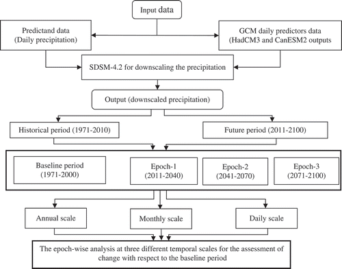
A schematic diagram showing the data used and methodology adopted is shown in Figure 1. A stepwise description is presented in the following sub-sections.

Figure 1. Schematic diagram of data used and the methodology adopted.

2.1 Study area

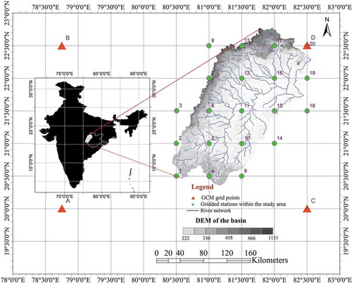
The upper part of the Mahanadi River Basin is considered as the study area (Fig. 2). As a major peninsular river of India, the Mahanadi River flows from west to east. It is the seventh largest river in India with several important tributaries, such as Sheonath, Ib and Tel (Asokan and Dutta 2008). The study basin drains an area of 30 860 km². The study area is the most densely populated (282/km²) part of the Mahanadi Basin. The main river channel originates from a pool at an elevation of about 442 m a.m.s.l. The study area lies in the northeastern Deccan plateau between latitudes 20.16°N and 22.75°N and longitudes 80.5°E and 82.5°E. Rainfall is received principally from the summer monsoon, during the months of June to September. The average annual rainfall in the basin is 1463 mm/year. Rainfall is recorded as very low (approximately 15% to 20%) during the rest of the year.

Figure 2. Map showing the Mahanadi Basin (key map) and the Upper Mahanadi Basin (UMB, highlighted and enlarged). Gridded locations for downscaling grid intersections (circles) and GCM grid intersections (triangles) are also shown in the enlarged UMB. Nine grid intersections are also considered for CanESM2, in which the study area is enclosed. These are not shown for clarity. A digital elevation model (DEM) of the study basin is shown in greyscale (m a.m.s.l.).

2.2 Data used

2.2.1 Local observed precipitation data (predictand)

Daily precipitation data at all the grid points shown in Figure 2 are obtained at a spatial resolution of 0.5° × 0.5° (latitude × longitude) from the India Meteorological Department (IMD). These daily rainfall data are available for 1971–2010. It is known that a sufficiently long data length is required to obtain a more or less stable estimate of the climate features for a given location (Trenberth 2008). In this study, 40 years (HadCM3) and 35 years (CanESM2) of data length are used as inputs for the SDSM. The first 20 years (1971–1990) of data are used for model calibration and the remaining 20 years (1991–2010) of data in the case of HadCM3 and 15 years (1991–2005) of data in the case of CanESM2 are used for model validation. The baseline period is considered as 1971–2000 when assessing climate change in the future (2011–2099 for HadCM3 and 2011–2100 for CanESM2).

2.2.2 Large-scale atmospheric variables (predictors)

The observed large-scale atmospheric variables are obtained from the National Centers for Environmental Prediction (NCEP) or National Center for Atmospheric Research (NCAR) (NCEP/NCAR) dataset for the period 1971–2010. The outputs of HadCM3 for A2 and B2 emissions scenarios, described in the Special Report on Emissions Scenarios (SRES) prepared by the IPCC, are used in this study. The NCEP/NCAR re-analysis data are re-gridded by the weighted average of neighbouring grid points, as HadCM3 contains a grid spacing of 2.5° latitude and 3.75° longitude, whereas NCEP/NCAR re-analysis data have grid sizes of latitude 2.5° and longitude 2.5°. These re-gridded NCEP/NCAR predictors are used as input to run the SDSM model. These standardized predictor variables are also supplied by the Canadian Climate Impacts Scenarios Group (http://www.cics.uvic.ca/scenarios/sdsm/select.cgi). The predictor variables for CanESM2 are downloaded from the Coupled Model Intercomparison Project – phase 5 (CMIP5). These predictor variables are available at http://www.ipcc-data.org/sim/gcm_monthly/AR5/Reference-Archive.html.

2.3 Model description and execution

The SDSM involves a hybrid of the stochastic weather generator and multi-regression-based methods (Wilby and Dawson 2013). It establishes linear relationship between large-scale atmospheric variables (predictors) and small-scale surface variables (predictands) (Wilby 1998, Wilby et al. 2002, Meenu et al. 2013, Pervez and Henebry 2014). The model is set up separately for each of the 20 locations shown in Figure 2. The GCM variables at the required locations are obtained by applying the inverse distance weighting (IDW) method on the GCM data from four nearest neighbouring grid points. In the case of HadCM3, four GCM grids, and in the case of CanESM2, nine GCM grids are found to be necessary to cover all the grid points in the study basin. The variables interpolated through the IDW method are used as inputs to the SDSM for each location.

The procedure of downscaling follows Wilby et al. (2002). The procedure starts with the Quality Control step, in which the quality of the predictand (precipitation in this study) is checked. The Quality Control step provides information about missing values, identification of which is very important in determining the quality of input data. However, there are no missing values in the data used in this analysis. The fourth root transform (available in the Transform Data screen in the SDSM) is applied to the original time series of observed precipitation in order to convert it to a normal distribution (to be used in the regression analysis). The predictors are selected from the Screen Variables step based on the results of seasonal correlation analysis, partial correlation analysis and scatter plots. In this step, a maximum of 12 predictor variables can be selected in a single run. In this study, separate analyses are performed at the monthly, seasonal and annual scales in order to identify the best predictors. Consequently, the correlation between the predictors and predictand are obtained from the Screen Variables window. The predictors that possess good correlation with the predictand are selected in this step. For brevity, the correlation coefficients are not presented in this paper. The next step in the SDSM is Calibrate Model, in which the model is calibrated by considering the first 20 years of daily data. It is important to note that in the Calibrate Model step, the “conditional” process is selected because local precipitation correlates with the occurrence of wet days (Wilby and Dawson 2013).

The predictors that are finalized in the Screen Variables step are selected in the Calibrate Model step. In this step, the SDSM develops a relationship between the predictors and the predictand by computing the parameters of multiple regression equations via the ordinary least squares optimization technique. The downscaled synthetic daily precipitation time series is produced in the Scenario Generator step by using the GCM predictors obtained from the HadCM3 and CanESM2. The future daily precipitation time series events are downscaled by using the A2 and B2 scenario predictors for HadCM3, and RCP 4.5 for CanESM2, for all the locations. In the case of HadCM3 a year is considered to be 360 days long, whereas in the case of CanESM2 it is considered to be 365 days. Therefore, the “year length” is selected accordingly. Further analyses are carried out on the future downscaled precipitation by categorizing the results into three defined time spans, named “epochs”, as follows: epoch-1 (2011–2040), epoch-2 (2041–2070) and epoch-3 (2071–2099 for HadCM3 and 2071–2100 for CanESM2).

2.4 Bias correction

The main sources of uncertainty in downscaling analysis are location, scenario, GCM and downscaling technique. The uncertainty originating from the location can be physically consistent, whereas uncertainty from any other source can lead to incorrect results (Sobie et al. 2013). The confidence in the consistency of the climate change anomalies computed from the scenario runs depends on the ability of the downscaled outputs to represent the baseline climate (Dibike et al. 2008). We evaluated the performance of the downscaling method in reproducing the mean and variability of the observed precipitation by comparing downscaled precipitation obtained from climate predictors with observed precipitation records for 1971–2000 (baseline period). Based on the discrepancy, bias correction factors are computed for each month. These factors are multiplied by the future downscaled monthly precipitation values to obtain the bias corrected precipitation values. Thereafter, the corrected daily precipitation values are also determined by using the same bias correction factors before assessment of any change. The bias corrected precipitation values are referred as simply “downscaled precipitation” henceforth in this paper.

2.5 Model evaluation criteria

The downscaled precipitation is analysed on the monthly scale and the performance of the SDSM model is evaluated through the Nash-Sutcliffe efficiency (NSE), the coefficient of determination (R²) and root mean square error (RMSE). The NSE indicates a normalized statistics that determines the relative magnitude of the residual variance compared to the measured data variance (Nash and Sutcliffe 1970). The NSE varies from −∞ to 1.0 (including 1.0); values between 0.0 and 1.0 are acceptable while values less than zero indicate prediction performance worse than the mean. The maximum possible value of NSE is 1.0, which indicates a perfect model. The RMSE represents the difference between modelled (downscaled) daily precipitation values and observed daily precipitation values. It generally indicates the error component between predicted and observed data. The coefficient of determination (R²) represents the closeness among the observed and modelled values.

3 Results and discussion

3.1 Identification of predictors

The predictors were identified based on the correlation coefficient between predictors and predictand. The frequency of use (i.e. for how many out of the 20 locations the particular predictor has been utilized) of the predictor variables in the study basin is represented in Table 1. It is observed that out of 26 predictor variables, 13 are found to be useful for downscaling the precipitation in the study area (Table 1). Specifically, mean sea level pressure (MSLP), geopotential height at 500 hPa pressure level, zonal velocity at 500 hPa and specific humidity at 1000 hPa pressure level showed good relations with precipitation. This finding is also supported by previous studies. For instance, considerable association between precipitation and geopotential height is identified (Saeed et al. 2012). The meridional wind velocity is also found to significantly influence all India monsoonal precipitation (Bawiskar et al. 2005). In this study, the MSLP, zonal velocity, meridional velocity, geopotential height and specific humidity were found to be the principal predictors for the study basin.

Table 1. Predictor variables from NCEP re-analysis and HadCM3 datasets, and frequency of being selected based on high correlation coefficient with observed precipitation in the Upper Mahanadi Basin.

Predictor code	Description	Frequency of use
mslp	Mean sea level pressure	18/20
P5_u	500 hPa zonal velocity	18/20
P500	500 hPa geopotential height	18/20
shum	1000 hPa specific humidity	17/20
P8_v	850 hPa meridional velocity	17/20
r850	850 hPa relative humidity	17/20
P850	850 hPa geopotential height	16/20
P_u	1000 hPa zonal velocity	12/20
P5th	500 hPa wind direction	10/20
P5_v	500 hPa meridional velocity	8/20
r500	500 hPa relative humidity	3/20
P_v	1000 hPa meridional velocity	2/20
P8th	850 hPa wind direction	1/20

3.2 Calibration and validation of SDSM

The calibration and validation of SDSM 4.2 through observed and downscaled daily precipitation time series is carried out for all the locations shown in Figure 2. For brevity, only results for location 12 are presented (Fig. 3 for HadCM3 and Fig. 4 for CanESM2). In these figures, panels a and b represent the time series of downscaled precipitation and observed precipitation at daily and monthly scales, respectively, while panel c shows the scatter plot between observed and downscaled precipitation during the calibration period. It is found that the downscaled precipitation corresponds well to the observed precipitation during the calibration period. The statistical measures (R² = 0.757, NSE = 0.745, and RMSE = 1.935 mm) obtained during the calibration period of HadCM3 were reasonably good at the monthly scale. In the case of CanESM2, R² of 0.733, NSE of 0.652 and RMSE of 2.450 mm are observed during the same period. However, at the daily scale, some of the extremes are not captured. Further analysis at the daily scale is presented later.

Figure 3. Calibration and validation results of statistical downscaling model (SDSM) with NCEP re-analysis predictors for location 12, marked in Figure 2. Observed and downscaled precipitation during calibration at (a) the daily scale and (b) the monthly scale. (c) Scatter plot at the monthly scale during calibration (RMSE: 1.935 mm, R²: 0.757, and NSE: 0.745). Observed and downscaled precipitation during validation at (d) the daily scale and (e) the monthly scale. (f) Scatter plot at the monthly scale during validation (RMSE: 1.976 mm, R²: 0.780, NSE: 0.753).

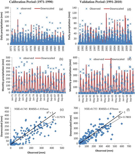
Figure 4. Calibration and validation results of SDSM at location 12, marked in Figure 2 using CanESM2 outputs. Observed and downscaled precipitation during calibration at (a) the daily scale and (b) the monthly scale. (c) Scatter plot at the monthly scale during calibration (RMSE: 2.450 mm, R²: 0.733, and NSE: 0.652). Observed and downscaled precipitation during validation at (d) the daily scale and (e) the monthly scale. (f) Scatter plot at the monthly scale during validation (RMSE: 2.240 mm, R²: 0.764, NSE: 0.719).

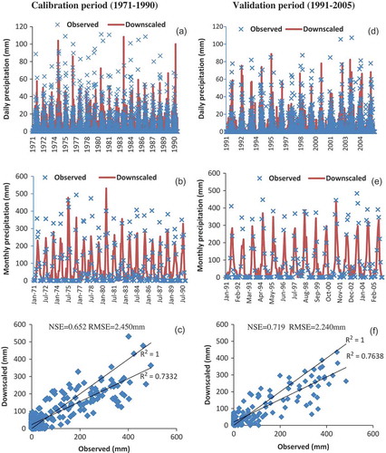
In Figures 3 and 4, panels d and e represent the time series of downscaled precipitation and observed precipitation at daily and monthly scales, respectively, for the validation period. Panel c shows the scatter plot between observed and downscaled precipitation during the same period. Validation of the model using HadCM3 reveals values for R² of 0.780, NSE of 0.753 and RMSE of 1.976 mm. In the case of CanESM2, values for R² of 0.764, NSE of 0.719 and RMSE of 2.240 mm are noted during the same period. It is found that the downscaled precipitation corresponds well to the observed precipitation during calibration and validation periods for both HadCM3 and CanESM2.

The same procedure is followed for the remaining 19 locations. The performance statistics (R², NSE and RMSE) are captured for all these locations for HadCM3 and CanESM2 and reported in Tables 2 and 3, respectively. It can be noted that the correlation coefficient (R²) is found to be a minimum of 0.598 (at location 3) from Table 2 in the case of HadCM3 and 0.602 (location 9) from Table 3 in the case of CanESM2. The maximum value of R² is obtained as 0.773 (at location 19) from Table 2 in the case of HadCM3 and 0.733 (at location 12) from Table 3 in the case of CanESM2. From this analysis, it is clear that the spatial pattern of the precipitation is changing from location to location. The results are more or less consistent at all the locations. Thus, the calibrated/validated SDSM is used for downscaling the future precipitation.

Table 2. Statistical performance measures between observed and downscaled (by SDSM) precipitation for the calibration and validation periods at all locations using HadCM3 outputs as input to SDSM.

		Calibration			Validation
Location no.	Location	RMSE (mm)	R^2	NSE	RMSE (mm)	R^2	NSE
1	20.5°N, 80.5°E	2.82	0.61	0.58	3.11	0.64	0.63
2	21.0°N, 80.5°E	2.92	0.64	0.61	2.99	0.66	0.65
3	21.0°N, 80.5°E	3.24	0.60	0.57	3.16	0.60	0.58
4	20.5°N, 81.0°E	3.06	0.71	0.71	3.08	0.70	0.69
5	21.0°N, 81.0°E	2.81	0.67	0.67	2.94	0.64	0.60
6	21.5°N, 81.0°E	2.05	0.71	0.69	2.05	0.67	0.58
7	22.0°N, 81.0°E	2.41	0.71	0.68	2.43	0.68	0.67
8	22.5°N, 81.0°E	3.13	0.65	0.57	2.98	0.66	0.61
9	20.5°N, 81.5°E	2.72	0.64	0.64	2.86	0.67	0.64
10	21.0°N, 81.5°E	2.42	0.67	0.70	2.41	0.70	0.70
11	21.5°N, 81.5°E	2.37	0.68	0.66	2.37	0.76	0.74
12	22.0°N, 81.5°E	1.94	0.76	0.75	1.98	0.78	0.75
13	22.5°N, 81.5°E	2.27	0.75	0.74	1.64	0.81	0.79
14	21.0°N, 82.0°E	3.17	0.72	0.69	2.96	0.69	0.67
15	21.5°N, 82.0°E	2.40	0.72	0.70	2.36	0.69	0.66
16	22.0°N, 82.0°E	2.47	0.70	0.70	2.16	0.75	0.74
17	22.5°N, 82.0°E	2.31	0.75	0.74	2.11	0.74	0.71
18	21.5°N, 82.5°E	3.05	0.68	0.64	3.22	0.67	0.65
19	22.0°N, 82.5°E	2.40	0.77	0.77	2.73	0.66	0.64
20	22.5°N, 82.5°E	2.34	0.73	0.71	2.15	0.78	0.74

Table 3. Statistical performance measures between observed and downscaled (by SDSM) precipitation for the calibration and validation periods at different locations using CanESM2 outputs as input to SDSM.

		Calibration			Validation
Location no.	Location	RMSE (mm)	R^2	NSE	RMSE (mm)	R^2	NSE
1	20.5°N, 80.5°E	3.29	0.65	0.62	3.21	0.66	0.64
2	21.0°N, 80.5°E	3.12	0.61	0.60	2.90	0.64	0.63
3	21.0°N, 80.5°E	2.86	0.68	0.66	3.17	0.61	0.61
4	20.5°N, 81.0°E	3.18	0.70	0.65	3.24	0.67	0.64
5	21.0°N, 81.0°E	3.12	0.62	0.61	2.83	0.69	0.67
6	21.5°N, 81.0°E	2.43	0.65	0.61	2.62	0.62	0.58
7	22.0°N, 81.0°E	2.03	0.70	0.70	2.31	0.68	0.62
8	22.5°N, 81.0°E	2.83	0.71	0.64	3.16	0.68	0.65
9	20.5°N, 81.5°E	3.05	0.60	0.60	2.87	0.70	0.62
10	21.0°N, 81.5°E	2.66	0.62	0.61	2.48	0.67	0.62
11	21.5°N, 81.5°E	2.43	0.65	0.62	2.17	0.68	0.66
12	22.0°N, 81.5°E	2.45	0.73	0.65	2.24	0.76	0.72
13	22.5°N, 81.5°E	2.73	0.70	0.65	2.56	0.69	0.68
14	21.0°N, 82.0°E	2.97	0.68	0.60	2.87	0.70	0.62
15	21.5°N, 82.0°E	2.63	0.67	0.59	2.47	0.70	0.62
16	22.0°N, 82.0°E	3.11	0.68	0.61	3.00	0.70	0.63
17	22.5°N, 82.0°E	2.86	0.71	0.62	2.37	0.74	0.69
18	21.5°N, 82.5°E	2.97	0.62	0.61	2.68	0.67	0.61
19	22.0°N, 82.5°E	2.98	0.66	0.59	2.67	0.73	0.66
20	22.5°N, 82.5°E	3.02	0.70	0.65	2.89	0.74	0.69

3.3 Bias correction of downscaled precipitation

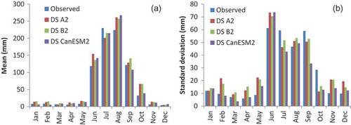
It is necessary to identify the skill of the GCM in simulating the observed values. A comparison between observed and downscaled precipitation will derive bias correction factors. These factors are obtained by dividing the observed monthly precipitation by the downscaled monthly precipitation. The bias correction factors are calculated for each month separately based on all 20 locations and 40 years of observed data. Month-wise bias correction factors for HadCM3 (both A2 and B2 scenarios) and CanESM2 are presented in Table 4. They are found to be random across monsoon and non-monsoon months. This is perhaps due to the inability of these GCMs to model the variations of precipitation and to represent long-term persistence in precipitation records in this region. The bias correction factors are expected to take care of this issue to some extent. Further investigation reveals that these factors are close to 1 (approximately 0.78 to 1.15) in the monsoon months of HadCM3 (for both the scenarios), whereas they vary from 0.48 to 0.85 in non-monsoon months. In the case of CanESM2, the range of these factors is found to be 0.83–1.12 during monsoon months and 0.54–1.52 during non-monsoon months. Thus, the precipitation is underestimated in some months and overestimated in others. The same can be observed from Figure 5(a), which shows the monthly means of observed and downscaled precipitation for the A2 and B2 scenarios of HadCM3 (during 1971–2010) and CanESM2 (during 1971–2005). The standard deviations for the same period for observed and downscaled precipitation for both the GCMs are shown in Figure 5(b). It is observed that the monthly mean (panel a) of the downscaled precipitation is underestimated during the month of July and overestimated during the other monsoon months (June, August and September). The month-wise standard deviations (panel b) of the downscaled precipitation also vary from month to month, showing both underestimation and overestimation across different months of the year. Therefore, to match the downscaled precipitation with the observed precipitation, the month-wise bias correction factors are multiplied by the downscaled monthly precipitations before assessing the performance of the models.

Table 4. Month-wise bias correction factors for HadCM3 A2 and B2 scenarios and CanESM2.

	HadCM3 Scenarios
Month	A2	B2	CanESM2
January	0.58	0.53	1.35
February	0.66	0.56	1.52
March	1.02	0.64	0.74
April	0.48	0.63	0.56
May	0.49	0.52	0.61
June	0.79	0.87	0.83
July	1.14	1.07	1.07
August	0.86	0.87	0.84
September	0.95	0.86	1.12
October	0.49	0.49	0.83
November	0.45	0.49	0.57
December	0.78	0.74	0.54

Figure 5. Annual cycles of Upper Mahanadi Basin precipitation averaged over the entire basin for the period 1971–2010 using downscaled A2 (DS A2) and downscaled B2 (DS B2) scenarios and for 1971–2005 using downscaled CanESM2 (DS CanESM2): (a) observed and downscaled monthly averaged precipitation and (b) standard deviation.

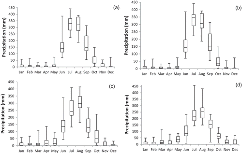
To assess the performance of the model at the monthly scale, box plots are prepared between observed and downscaled precipitation. Five different horizontal lines (top to bottom) in a box plot represent the maximum, third quartile, median, first quartile and minimum monthly precipitation values during 1971–2010. The box plots shown in Figure 6 represent the performance of the SDSM at the monthly scale. In Figure 6, panels a, b, c and d represents observed precipitation, downscaled A2 precipitation, downscaled B2 precipitation and downscaled CanESM2 precipitation, respectively. The performance of the SDSM is satisfactory in representing the medians during monsoon months for both A2 and B2 scenarios of HadCM3 and CanESM2. However, the performance of the model is poor during the months of January and February, where the downscaled average precipitation is very low as compared to the observed average precipitation. The similarity between annual observed precipitation and annual downscaled precipitation is checked by calculating the annual average value of downscaled precipitation. It is observed that the downscaled precipitation matches well with observed annual precipitation. However, there might be some month-wise discrepancies.

Figure 6. Box plots of (a) observed, (b) downscaled HadCM3 A2 scenario and (c) downscaled HadCM3 B2 scenario precipitation distributions for all locations in the study basin during the period 1971–2010. (d) Downscaled CanESM2 precipitation distribution for the study basin during the period 1971–2005.

In the case of daily precipitation, depending on the corresponding month, the bias correction factors are multiplied by the daily precipitation to obtain the bias corrected daily precipitation time series. After the bias correction, the future precipitation patterns are compared with the baseline, presented in the next section.

3.4 Assessment of climate change effect in comparison with baseline period

3.4.1 Assessment of change at monthly scale

From the previous downscaling studies it is clear that precipitation will increase in the future. Pervez and Henebry (2014) found that future precipitation will increase by 10.4–12.5% in the Ganges Basin during 2076–2100. Similarly, the amount of precipitation will increase by 11.8–16.1% during the same period in the Brahmaputra Basin. A similar increasing trend was also reported by Meenu et al. (2013) in the Tunga-Bhadra River Basin of Southern India.

In this section, month-wise variation of precipitation in the future is analysed. The future precipitation is projected in the study basin for HadCM3 (A2 and B2 scenarios) and CanESM2 (RCP4.5) during the 21st century. The future period is divided into three epochs (30 years each) – epoch-1 (2011–2040), epoch-2 (2041–2070) and epoch-3 (2071–2100). The results for all the epochs are presented in Figure 7. The results are compared to the baseline period (1971–2000). It is found that the precipitation increases gradually from epoch-1 to epoch-3. More precisely, an overall increase in annual precipitation by 10.0% and 12.0% is observed during epoch-2 and epoch-3, respectively, in the case of the A2 scenario. In the case of the B2 scenario, annual precipitation increases by 10.4% and 12.1% during epoch-2 and epoch-3, respectively. In the case of CanESM2 (RCP 4.5), the increase in annual precipitation is calculated as 8.3% and 11.6%, respectively, during the same epochs. The results are further analysed to check the increase in monthly precipitation during monsoon months (June through September) and non-monsoon months (October through May). During the monsoon months, the increase is found to be 9.2% and 11.3% in the case of the A2 scenario during epoch-2 and epoch-3, respectively. In the case of the B2 scenario, for the same epochs, the increase is 10.2% and 11.5% during the monsoon months, respectively. When considering CanESM2 (RCP 4.5) data, the increases in monthly precipitation during the monsoon months of epoch-2 and epoch-3 are 10.7% and 13.0%.

Figure 7. Comparison of downscaled precipitation with baseline (1971–2000) precipitation: (a) HadCM3 (A2 scenario) precipitation, (b) HadCM3 (B2 scenario) precipitation and (c) CanESM2 (RCP 4.5) precipitation.

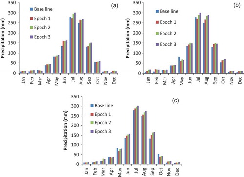
During the non-monsoon months, the increases in monthly precipitation corresponding to epoch-2 and epoch-3 are found to be 12.9% and 14.5% (HadCM3, A2 scenario), 11.3% and 14.4% (HadCM3, B2 scenario) and 9.8% and 11.2% (CanESM2, RCP4.5), respectively. Increases in precipitation are observed in most of the monsoon months for both the GCMs. However, in the case of July, a decreasing trend is observed till epoch-1 in the A2 and B2 scenarios of HadCM3 and an increasing trend thereafter. In the case of CanESM2 (RCP 4.5), there is gradual increase in the precipitation over the 21st century during all the monsoon months (panel c of Fig. 7). However, monthly analysis does not reveal information on any change in daily extremes. Assessment of daily extremes is carried out in the next section.

3.4.2 Assessment of change in daily extremes

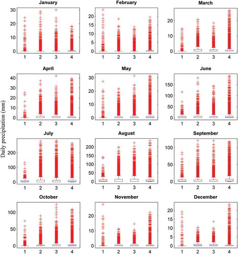
The changes in the daily extremes are important for various applications. However, the day-to-day variation of precipitation obtained from SDSM is not as reliable in practice as the results obtained at the monthly scale (Pervez and Henebry 2014). It is indeed true that the day-to-day variation of precipitation may not be meaningful in the future (after 50–100 years). Rather, in this section, an attempt is made to extract the information on the changes in daily extremes likely to occur in the future (different epochs) as compared to the baseline period. It is obvious that such changes are expected to vary spatio-temporally, i.e. they will change from one epoch to another (temporal) as well as one location to another (spatial). For demonstration purposes, location 12 (Fig. 2) and epoch-3 are considered to assess the change in daily extreme precipitation as compared to the baseline period. In Figure 8, box plots with whiskers for daily precipitation are shown separately for each month for observed precipitation during the baseline period and the bias corrected, downscaled, future precipitation for both HadCM3 and CanESM2. It may be noted that a whisker is a value in a dataset that is “sufficiently” far away from the interquartile range. In this study, a whisker is defined as the data points that are either larger than or smaller than , where and are the 25th and 75th quantile data, respectively. It is noted from Figure 8 that the daily extremes are likely to increase in most months except for a few non-monsoon months. Analyses are also carried out for the individual months to examine the daily extremes during epoch-3. The results reveal that there is a mixed response in the non-monsoon months. The numbers of daily extremes are increasing in the pre-monsoon months of January, March and April, but decreasing slightly in February and May. During the monsoon months (June, July, August and September), the numbers of daily extremes are increasing for both the GCMs as compared to the baseline period (see Fig. 8). In the post monsoon months, October shows an increasing trend but November and December show a decrease in daily extremes for both the scenarios of HadCM3 when compared to the baseline period. In the case of CanESM2 (RCP 4.5), a decrease in daily extremes is found for November. In general, the results indicate that extreme rainfall events are going to increase in future epochs. Although the numbers of extreme events seem to be decreasing during November and December, the magnitudes of the 75th quantiles are increasing in both months as compared to the baseline period for both the GCMs. This necessitates further detailed monthly-level analysis on the daily extremes, which is presented in the next section.

Figure 8. Daily extremes for all months between observed precipitation during the baseline period (1971–2000), bias corrected, downscaled precipitation for HadCM3 A2 and B2 emissions scenarios for epoch-3 (2071–2099) and CanESM2 (RCP4.5) for epoch-3 (2071–2100), respectively shown as 1, 2, 3 and 4 on the x-axis. The boxes represent the 25th, 50th and 75th quantiles.

In order to quantify the change in daily precipitation, two different approaches are followed. In the first approach, the value corresponding to the 95th quantile of daily precipitation is obtained for the observed precipitation and projected precipitation. These values are shown in Table 5. It is observed from the table that there is a clear increasing trend of extreme rainfall in the future. The 95th quantile value in the baseline period (17.26 mm) rises to 24.31, 24.48 and 23.51 mm in the A2 and B2 scenarios of HadCM3 and CanESM2 (RCP 4.5), respectively, during epoch-3. The analysis is further continued for individual months to identify the frequency of occurrence of precipitation during the future epochs. For individual months, the 95th quantile values during the baseline period and future epochs for both GCMs are obtained and the results are listed in Table 6. It can be observed that the 95th quantile values during the future epochs are higher in all months except February when compared to the baseline period.

Table 5. Precipitation magnitude (in mm) corresponding to the 95th quantile for baseline and future epochs.

	Projected future precipitation
	HadCM3
	A2 scenario			B2 scenario			CanESM2
Baseline	Epoch-1	Epoch-2	Epoch-3	Epoch-1	Epoch-2	Epoch-3	Epoch-1	Epoch-2	Epoch-3
17.26	22.88	24.14	24.31	23.05	24.25	24.48	21.35	22.01	23.51

Table 6. Month-wise variation of 95th quantile of daily precipitation (in mm).

		A2 scenario			B2 scenario			Can ESM2
Month	Observed	Epoch-1	Epoch-2	Epoch-3	Epoch-1	Epoch-2	Epoch-3	Epoch-1	Epoch-2	Epoch-3
January	2.26	2.75	2.83	2.71	2.39	2.72	2.13	2.17	2.15	2.22
February	2.37	2.26	2.31	2.21	1.92	2.00	1.95	2.36	2.39	2.33
March	1.58	4.70	4.79	4.67	3.64	3.62	3.70	5.01	4.70	5.44
April	1.27	7.66	8.07	7.42	6.81	6.58	6.79	6.74	6.98	7.09
May	2.29	4.39	4.70	4.40	5.28	5.51	5.21	6.24	6.79	7.10
June	22.26	40.07	40.07	39.60	46.82	46.81	44.12	28.50	30.76	36.54
July	34.69	76.95	79.68	80.32	81.49	82.95	83.9	43.84	48.80	58.41
August	38.05	56.86	56.45	55.04	54.12	56.01	53.41	38.77	44.22	50.35
September	21.56	36.46	37.84	38.89	35.31	35.63	34.27	27.53	30.90	32.91
October	9.21	17.31	17.36	15.71	19.12	19.16	19.97	16.35	17.69	21.21
November	2.07	2.64	2.59	2.49	2.58	2.56	2.59	3.20	3.00	3.73
December	0.71	2.91	2.84	2.84	3.44	3.37	3.63	2.351	2.50	2.76

In the second approach, the change in the number of days having extreme precipitation is computed. First, the number of days having precipitation higher than the 95th quantile value (i.e. 17.26 mm) is recorded for the baseline period. Such events are denoted as “extreme events” hereafter. Since the total number of “available” days is not the same in the baseline period and in the different epochs, extreme events are counted as “out of 100 events” in all cases, i.e. baseline period, epochs 1, 2 and 3. It is obvious that for the baseline period the count will be 5 out of 100 since the 95th quantile of the baseline period itself is considered. However, there could be some numerical error arising due to countable sample size. Compared to the baseline, the number of daily extreme events is found to increase in the future. The number of daily extreme events in a year is increased to 6.71, 6.64 and 7.02 (out of 100) for epochs 1, 2 and 3, respectively, in the case of the A2 emissions scenario. For the B2 emissions scenario, the values are 6.57, 6.71 and 7.04 for epochs 1, 2 and 3, respectively. Analysis with the data from CanESM2 (RCP 4.5) also indicates a similar trend—the number of daily extreme events is 6.24, 6.37 and 6.83 for epochs 1, 2 and 3, respectively.

The month-wise events (expressed as a percentage) with rainfall higher than the observed 95th quantile are shown in Table 7 for all the scenarios and both GCMs. From the month-wise analysis, it is found that there will be more rainy days in future in most months. The percentage increase in the number of rainy days is even greater during the pre- and post-monsoon months (i.e. March–May, October and December) as compared to the monsoon months (June–September). Therefore, the non-monsoon months may become wetter with respect to the baseline period. An increase in the number of rainy days is also evident for the monsoon months in the future, though the percentage increase is lower than for the non-monsoon months. Overall, daily extreme events are more likely to occur in the study basin during the 21st century, as compared to the baseline period (1971–2000). The results at the remaining locations indicate an almost similar trend.

Table 7. Number of events with rainfall greater than the baseline 95th quantile value (in %).

		A2 scenario			B2 scenario			CanESM2
Month	Observed	Epoch-1	Epoch-2	Epoch-3	Epoch-1	Epoch-2	Epoch-3	Epoch-1	Epoch-2	Epoch-3
January	5.05	5.80	6.00	6.16	5.28	5.84	5.01	4.79	4.71	4.89
February	5.00	4.73	5.12	4.80	3.98	4.18	4.10	4.99	5.23	4.92
March	5.05	21.17	20.89	20.23	16.41	15.82	16.28	14.50	13.37	14.70
April	5.00	27.47	29.02	26.55	24.44	24.24	24.16	19.64	19.42	20.70
May	5.05	11.74	12.57	11.71	13.60	14.48	13.32	13.12	14.05	15.05
June	5.00	14.10	15.13	14.37	14.50	15.11	13.21	6.69	7.20	8.85
July	5.05	16.31	16.87	17.22	16.36	16.52	14.57	6.74	7.29	9.03
August	5.05	9.99	10.09	9.26	9.09	9.44	9.15	5.15	6.11	6.77
September	5.00	10.89	11.28	11.70	10.09	10.93	10.44	6.70	7.53	9.13
October	5.05	11.17	10.86	10.28	11.77	12.45	13.01	8.77	9.68	12.07
November	5.00	7.71	7.24	7.17	7.13	7.28	7.49	7.74	7.39	8.68
December	4.85	28.47	28.79	28.43	27.41	26.09	27.74	13.24	13.98	15.42

4 Summary and conclusions

Future precipitation trends, in terms of annual totals, monthly variation and change in daily extremes, over the upper part of Mahanadi Basin are investigated in this study. Bias corrected, downscaled precipitation at a resolution of 0.5° × 0.5° over the basin is analysed for three future epochs (2011–2040, 2041–2070, 2071–2100) and contrasted with the baseline period (1971–2000). The SDSM 4.2 was used to downscale the precipitation using the atmospheric predictors from GCMs (HadCM3 and CanESM2). The predictors are selected based on significant correlation between the predictor and predictand. It is noticed that the precipitation over the study basin at different grid intersections is mostly influenced by the MSLP, zonal wind velocity (500, 850 and 1000 hPa), geopotential height (500 and 850 hPa) and specific humidity (1000 hPa). However, relative humidity at 850 hPa and 850 hPa meridional velocities is also important for some locations.

At the three temporal scales, the following major findings are noted from this study:

• At the annual scale, it is found that precipitation is likely to increase gradually from epoch-1 to epoch-3, and the increase is projected to be 10% and 12% for epoch-2 and epoch-3, respectively, in the case of the A2 emissions scenario. For the B2 scenario, the increase is projected to be 10% and 12%, respectively, for the same epochs. The increase is 7% and 11% for the corresponding epochs in the case of CanESM2 (RCP 4.5).

• For monthly precipitation, the results indicate that the precipitation totals are likely to increase in almost all months of the year in the future. The magnitude of the increase is higher during monsoon months and lower during non-monsoon months. However, the maximum percentage increase with respect to the baseline period occurs in the post-monsoon months (November–February) as compared to pre-monsoon (March–May) and monsoon months.

• In the case of daily analyses, the 95th quantiles of daily rainfall magnitude are projected to increase in the future in most months in the year. The increase is greater during the monsoon months as compared to non-monsoon months. It is also noticed that the number of extreme events (rainfall magnitude more than the 95th quantile of the observed value in the baseline period) is projected to increase in all months except February. However, the maximum increase (with respect to the situation in the baseline period) in the number of extreme events is observed in the non-monsoon months (specifically before and after the monsoon months).

• Comparison of monthly and daily analyses indicates that the total magnitude of monthly rainfall is expected to increase considerably in the monsoon months and slightly in the non-monsoon months. However, the percentage increase in the number of extreme events is expected to be higher in the non-monsoon months. Thus, it is expected that convective activity (precipitation) may increase in the non-monsoon months leading to a greater number of rainy days, particularly in the pre- and post-monsoon months.

As mentioned above, the limitation of the current study results from the inherent assumption of the application of the statistical downscaling technique for future climate scenarios. In the statistical downscaling method, it is assumed that the relationships between predictors (large-scale variables) and predictands (small-scale surface variables) do not change over time, which might be contradictory to the expected effect of climate change. In the present study, although the downscaled precipitations are bias corrected, the correction factors may be applied time-invariantly in the future. This limitation opens up future scope for a “time-varying” approach to the downscaling technique.

Disclosure statement

No potential conflict of interest was reported by the authors.

Additional information

Funding

This work was partially supported by the Ministry of Earth Sciences (MoES) (MoES/PAMC/H&C/30/2013-PC-II) through sponsored projects.

References

- Abdolhosseini, M., Eslamian, S., and Mousavi, S.F., 2012. Effect of climate change on potential evapotranspiration: a case study on Gharehsoo sub-basin, Iran. International Journal of Hydrology Science and Technology, 2 (4), 362–372. doi:10.1504/IJHST.2012.052373
- Arora, V.K. and Boer, G.J., 2010. Uncertainties in the 20th century carbon budget associated with land use change. Global Change Biology, 16 (12), 3327–3348. doi:10.1111/j.1365-2486.2010.02202.x
- Arora, V.K., et al., 2011. Carbon emission limits required to satisfy future representative concentration pathways of greenhouse gases. Geophysical Research Letters, 38, L05805. doi:10.1029/2010GL046270
- Asokan, S.M. and Dutta, D., 2008. Analysis of water resources in the Mahanadi River Basin, India under projected climate conditions. Hydrological Processes, 22, 3589–3603. doi:10.1002/hyp.v22:18
- Bárdossy, A., 1997. Downscaling from GCMs to local climate through stochastic linkages. Journal of Environmental Management, 49, 7–17. doi:10.1006/jema.1996.0112
- Bardossy, A. and Plate, E.J., 1992. Space-time model for daily rainfall using atmospheric circulation patterns. Water Resources Research, 28, 1247–1259. doi:10.1029/91WR02589
- Bawiskar, S.M., et al., 2005. Energetics of lower tropospheric planetary waves over mid latitudes: Precursor for Indian summer monsoon. Journal of Earth System Science, 114, 557–564. doi:10.1007/BF02702031
- Buishand, T.A. and Brandsma, T., 2001. Multisite simulation of daily precipitation and temperature in the Rhine basin by nearest-neighbor resampling. Water Resources Research, 37, 2761–2776. doi:10.1029/2001WR000291
- Changnon, S.A., Huff, F.A., and Hsu, C.-F., 1988. Relations between precipitation and shallow groundwater in Illinois. Journal of Climate, 1, 1239–1250. doi:10.1175/1520-0442(1988)001<1239:RBPASG>2.0.CO;2
- Chen, S.-T., Yu, P.-S., and Tang, Y.-H., 2010. Statistical downscaling of daily precipitation using support vector machines and multi variate analysis. Journal of Hydrology, 385, 13–22. doi:10.1016/j.jhydrol.2010.01.021
- Chu, J.T., et al., 2010. Statistical downscaling of daily mean temperature, pan evaporation and precipitation for climate change scenarios in Haihe River, China. Theoretical and Applied Climatology, 99, 149–161. doi:10.1007/s00704-009-0129-6
- Dibike, Y.B., et al., 2008. Uncertainty analysis of statistically downscaled temperature and precipitation regimes in Northern Canada. Theoretical and Applied Climatology, 91, 149–170. doi:10.1007/s00704-007-0299-z
- Du, J., et al., 2011. Precipitation change and human impacts on hydrologic variables in Zhengshui River Basin, China. Stochastic Environmental Research and Risk Assessment, 25, 1013–1025. doi:10.1007/s00477-010-0453-5
- Fiseha, B.M., et al., 2014. Impact of climate change on the hydrology of Upper Tiber River Basin using bias corrected regional climate model. Water Resources Management, 28, 1327–1343. doi:10.1007/s11269-014-0546-x
- Gagnon, S.B., et al., 2005. An application of the Statistical DownScaling Model (SDSM) to simulate climatic data for streamflow modelling in Québec. Canadian Water Resources Journal, 30 (4), 297–314. doi:10.4296/cwrj3004297
- Gain, A.K. and Wada, Y., 2014. Assessment of future water scarcity at different spatial and temporal scales of the Brahmaputra River Basin. Water Resources Management, 28, 999–1012. doi:10.1007/s11269-014-0530-5
- Ghosh, S. and Mujumdar, P.P., 2008. Statistical downscaling of GCM simulations to streamflow using relevance vector machine. Advances in Water Resources, 31, 132–146. doi:10.1016/j.advwatres.2007.07.005
- Gordon, C., Cooper, C., and Senior, C.A., 2000. The simulation of SST, sea ice extents and ocean heat transports in a version of the Hadley Centre coupled model without flux adjustments. Climate Dynamics, 16, 147–168. doi:10.1007/s003820050010
- Hewitson, B.C. and Crane, R.G., 1996. Climate downscaling : techniques and application. Climate Research, 7, 85–95. doi:10.3354/cr007085
- Jakeman, A.J. and Hornberger, G.M., 1993. How much complexity is warranted in a Rainfall-Runoff model? Water Resources Research, 29, 2637–2649. doi:10.1029/93WR00877
- Joshi, D., et al., 2016. Comparison of direct statistical and indirect statistical-deterministic frameworks in downscaling river low-flow indices. Hydrological Sciences Journal, 61, 1996–2010. doi:10.1080/02626667.2014.966719
- Kannan, S. and Ghosh, S., 2010. Prediction of daily rainfall state in a river basin using statistical downscaling from GCM output. Stochastic Environmental Research and Risk Assessment, 25, 457–474. doi:10.1007/s00477-010-0415-y
- Lee, M.-H. and Bae, D.-H., 2015. Climate change impact assessment on green and blue water over Asian Monsoon Region. Water Resources Management, 29, 2407–2427. doi:10.1007/s11269-015-0949-3
- Lombardo, F., Volpi, E., and Koutsoyiannis, D., 2012. Rainfall downscaling in time: theoretical and empirical comparison between multifractal and Hurst-Kolmogorov discrete random cascades. Hydrological Sciences Journal, 57 (6), 1052–1066. doi:10.1080/02626667.2012.695872
- Maraun, D., Wetterhall, F., and Iresson, A.M., 2010. Precipition downscaling under climate change: recent developments to bridge the gap between dynamical models and the end user. Reviews of Geophysics, 48, 1–34. doi:10.1029/2009RG000314
- Meenu, R., Rehana, S., and Mujumdar, P.P., 2013. Assessment of hydrologic impacts of climate change in Tunga – Bhadra river basin, India with HEC-HMS and SDSM. Hydrological Processes, 27, 1572–1589. doi:10.1002/hyp.v27.11
- Nash, J.E. and Sutcliffe, J.V., 1970. River flow forecasting through conceptual models part I — A discussion of principles. Journal of Hydrology, 10, 282–290. doi:10.1016/0022-1694(70)90255-6
- Pervez, M.S. and Henebry, G.M., 2014. Projections of the Ganges–Brahmaputra precipitation—Downscaled from GCM predictors. Journal of Hydrology, 517, 120–134. doi:10.1016/j.jhydrol.2014.05.016
- Pope, V.D., et al., 2000. The impact of new physical parametrizations in the Hadley Centre climate model: HadAM3. Climate Dynamics, 16, 123–146. doi:10.1007/s003820050009
- Reichler, T. and Kim, J., 2008. How well do coupled models simulate today’s climate? Bulletin of the American Meteorological Society, 89, 303–311. doi:10.1175/BAMS-89-3-303
- Sachindra, D.A., et al., 2014. Statistical downscaling of general circulation model outputs to precipitation – part 1 : calibration and validation. International Journal of Climatology, 34, 3264–3281. doi:10.1002/joc.3914
- Saeed, F., et al., 2012. Influence of mid-latitude circulation on Upper Indus basin precipitation: the explicit role of irrigation. Climate Dynamics, 40, 21–38. doi:10.1007/s00382-012-1480-3
- Salathe, E.P., 2003. Comparison of various precipitation downscaling methods for the simulation of streamflow in a rainshadow river basin. International Journal of Climatology, 23, 887–901. doi:10.1002/joc.922
- Schnorbus, M., Werner, A., and Bennett, K., 2014. Impacts of climate change in three hydrologic regimes in British Columbia, Canada. Hydrological Processes, 28, 1170–1189. doi:10.1002/hyp.v28.3
- Selker, J.S. and Haith, A., 1990. Development and testing of single-parameter precipitation distributions. Water Resources Research, 26, 2733–2740. doi:10.1029/WR026i011p02733
- Sobie, S.R., et al., 2013. Downscaling extremes: an intercomparision of multiple methods for future climate. Journal of Climate, 26, 3429–3449. doi:10.1175/JCLI-D-12-00249.1
- Solomon, S., 1967. Relationship between precipitation, evaporation, and runoff in tropical-equatorial regions. Water Resources Research, 3, 163–172. doi:10.1029/WR003i001p00163
- Srivastava, P.K., et al., 2015. WRF dynamical downscaling and bias correction schemes for NCEP estimated hydro-meteorological variables. Water Resources Management, 29, 2267–2284. doi:10.1007/s11269-015-0940-z
- Storch, H.V., Zorita, E., and Cubasch, U., 1993. Downscaling of global climate change estimates to regional scales: an application to Iberian Rainfall in wintertime. Journal of Climate, 6, 1161–1171. doi:10.1175/1520-0442(1993)006<1161:DOGCCE>2.0.CO;2
- Stott, P.A., et al., 2000. External control of 20th century temperature by natural and anthropogenic forcings. Science, 290, 2133–2137. doi:10.1126/science.290.5499.2133
- Tabor, K. and Williams, J.W., 2010. Globally downscaled climate projections for assessing the conservation impacts of climate change. Ecological Applications, 20, 554–565. doi:10.1890/09-0173.1
- Tisseuil, C., et al., 2010. Statistical downscaling of river flows. Journal of Hydrology, 385, 279–291. doi:10.1016/j.jhydrol.2010.02.030
- Tofiq, F.A. and Guven, A., 2014. Prediction of design flood discharge by statistical downscaling and general circulation models. Journal of Hydrology, 517, 1145–1153. doi:10.1016/j.jhydrol.2014.06.028
- Trenberth, K.E., 2008. Observational needs for climate prediction and adaptation. WMO Bulletin, 57 (1), 17–21.
- Tung, C. and Haith, D.A., 1995. Global-Warming effects on new york streamflows. Journal of Water Resources Planning and Management, 121, 216–225. doi:10.1061/(ASCE)0733-9496(1995)121:2(216)
- Wang, W., Xing, W., and Shao, Q., 2015. How large are uncertainties in future projection of reference evapotranspiration through different approaches? Journal of Hydrology, 524, 696–700. doi:10.1016/j.jhydrol.2015.03.033
- Wang, W., et al., 2013. Changes in reference evapotranspiration across the Tibetan Plateau: observations and future projections based on statistical downscaling. Journal of Geophysical Research: Atmospheres, 18 (10), 4049–4068.
- Wang, W., et al., 2014. Responses of rice yield, irrigation water requirement and water use efficiency to climate change in China: historical simulation and future projections. Agricultural Water Management, 146, 249–261. doi:10.1016/j.agwat.2014.08.019
- Wilby, R.L., 1998. Statistical downscaling of daily precipitation using daily airflow and seasonal teleconnection indices. Climate Research, 10, 163–178. doi:10.3354/cr010163
- Wilby, R.L. and Dawson, C.W., 2013. The Statistical DownScaling Model: insights from one decade of application. International Journal of Climatology, 33, 1707–1719. doi:10.1002/joc.2013.33.issue-7
- Wilby, R.L., Dawson, C.W., and Barrow, E.M., 2002. SDSM — a decision support tool for the assessment of regional climate change impacts. Environmental Modelling & Software, 17, 145–157. doi:10.1016/S1364-8152(01)00060-3
- Wilby, R.L., et al., 2000. Hydrological responses to dynamically and statistically downscaled climate model output. Geophysical Research Letters, 27, 1199–1202. doi:10.1029/1999GL006078
- Wilby, R.L., Tomlinson, O.J., and Dawson, C.W., 2003. Multi-site simulation of precipitation by conditional resampling. Climate Research, 23, 183–194. doi:10.3354/cr023183
- Wilby, R.L. and Wigley, T.M.L., 1997. Downscaling general circulation model output: a review of methods and limitations. Progress in Physical Geography, 21, 530–548. doi:10.1177/030913339702100403
- Yang, T., et al., 2012. Statistical downscaling of extreme daily precipitation, evaporation, and temperature and construction of future scenarios. Hydrological Processes, 26 (23), 3510–3523. doi:10.1002/hyp.v26.23