Water temperature modelling: comparison between the generalized additive model, logistic, residuals regression and linear regression models

ABSTRACT

Water temperature has a significant influence on aquatic organisms, including stenotherm fish such as salmonids. It is thus of prime importance to build reliable tools to forecast water temperature. This study evaluated a statistical scheme to model average water temperature based on daily average air temperature and average discharge at the Sainte-Marguerite River, Northern Canada. The aim was to test a non-parametric water temperature generalized additive model (GAM) and to compare its performance to three previously developed approaches: the logistic, residuals regression and linear regression models. Due to its flexibility, the GAM was able to capture some of the nonlinear response between water temperature and the two explanatory variables (air temperature and flow). The shape of these effects was determined by the trends shown in the collected data. The four models were evaluated annually using a cross-validation technique. Three comparison criteria were calculated: the root mean square error (RMSE), the bias error and the Nash-Sutcliffe coefficient of efficiency (NSC). The goodness of fit of the four models was also compared graphically. The GAM was the best among the four models (RMSE = 1.44°C, bias = −0.04 and NSC = 0.94).

KEYWORDS:

• mean daily water temperature
• logistic model
• generalized additive model (GAM)
• residuals regression
• linear regression

Editor M.C. Acreman; Associate editor S. Huang

1 Introduction

Water temperature is one of the physical factors controlling water quality. For instance, it affects oxygen concentration, which is inversely proportional to water temperature (Secondat 1952, Ozaki et al. 2003), as well as the concentration of some pollutants (Ficke et al. 2007). Water temperature has a direct or indirect effect on many other physical (e.g. density, viscosity), chemical (e.g. conductivity, oxygen solubility) or biological (Stevens et al. 1975) variables in lotic ecosystems.

The thermal regime of rivers is important for aquatic ecosystems (Cairns et al. 1978, Caissie 2006, Acuña and Tockner 2009). Water temperature is a determining ecological factor for many biological parameters such as metabolic activity (Demars et al. 2011), reproduction, survival (Eaton et al. 1995, Connor et al. 2003) and growth rate (Elliott and Hurley 1997, Neuheimer and Taggart 2007). Also, it has been proven that water temperature has an impact on the distribution of species in rivers (Magnuson et al. 1979, Vannote et al. 1980, Ebersole et al. 2003, Edwards and Cunjak 2007). Higher than average water temperatures may generate thermal stress for certain species of fish (Isaak et al. 2012). Indeed, the response to this stress for salmonids depends on the rate at which the water temperature increases (Quigley and Hinch 2006). In some cases, these species will seek thermal refuges, when available, in order to avoid being exposed to high-temperature conditions (Baird and Krueger 2003, Dugdale et al. 2013, Daigle et al. 2014).

Many studies focus on the identification of human impacts altering the thermal regimes of rivers. Some activities may have significant influence on water temperature, such as urbanization (e.g. Nelson and Palmer 2007), agriculture (e.g. Grégoire and Trencia 2007) and thermal effluents (e.g. Moatar and Gailhard 2006, Prats et al. 2012). Other important anthropogenic impacts include climate change, dams and logging. Climate change (CC) represents a significant threat to the life of aquatic species (Eaton and Scheller 1996, Mohseni et al. 2003, Webb et al. 2004, Crozier and Zabel 2006, Ferrari et al. 2007). Several studies have highlighted the fact that river water temperatures have increased significantly (Morrill et al. 2005, Ducharne 2008, Kaushal et al. 2010, Arismendi et al. 2012, Ficklin et al. 2013, Marszelewski and Pius 2015). Such a shift in the thermal regime of rivers would have a direct impact on the habitat conditions of poikilothermic organisms (Hari et al. 2006). The most notable ecological impact of CC remains the migration of different species to higher altitudes and latitudes, as a response to their thermal preferences (Walther et al. 2002, Parmesan and Yohe 2003). Changes in thermal signals due to the presence of reservoirs disrupt the life cycle of aquatic organisms (Lowney 2000). Indeed, dams alter the river thermal regime downstream of the impoundment (Webb 1996, Olden and Naiman 2010).

The modelling and forecasting of water temperatures under different spatial or temporal scales has conventionally been tackled using two models: deterministic and statistic (Caissie 2006, Benyahya et al. 2007, Cole et al. 2014). Deterministic or physical models are based on the mathematical representation of the physical processes of heat exchange between the river and its natural environment (Edinger et al. 1968, St-Hilaire et al. 2000, Caissie et al. 2007, Cox and Bolte 2007, Pike et al. 2013). They are typically developed at the river reach scale and are based on heat budget calculations, along with some degree of hydrological or hydrodynamic modelling. Although deterministic models can provide accurate estimates of water temperature, acquiring the necessary data is not always possible, especially at the regional level (Mohseni et al. 1998, Risley et al. 2003).

Statistical or empirical models remain an alternative that requires fewer parameters than deterministic models (Smith 1981, Mohseni et al. 2003, Morrill et al. 2005, Moore 2006, DeWeber and Wagner 2014). In addition to requiring less input data, statistical approaches often require a shorter period of development and reduced costs of data and operation (Eaton and Scheller 1996, Mohseni et al. 1999). However, they require long series of observations (Marceau et al. 1986). Statistical models do not take into account direct sources of heat flow. Instead, they represent the physical concept implicitly by taking into consideration the correlations between a relatively small number of input environmental variables and the water temperature (Caissie 2006, Webb et al. 2008). Multiple statistical works on water temperature modelling have already been presented, with their strengths and weaknesses (Benyahya et al. 2007). Among these statistical methods are the following:

(1) The parametric regression models, for which the relationship is parametrically specified a priori. This category includes the single or multiple linear regression, stochastic and nonlinear models (Smith 1981, Stefan and Preud’homme 1993, Erickson and Stefan 2000, Webb et al. 2003, Ahmadi-Nedushan et al. 2007) for predicting water temperature. They are more effective at weekly and monthly scales than at the daily scale, given that the daily water temperatures have greater autocorrelation (Pilgrim et al. 1998, Erickson and Stefan 2000, Morrill et al. 2005, Caissie 2006). The term “stochastic model” has been used to describe water temperature models that decompose time series into a seasonal and a residual component so as to produce daily forecasts of water temperature (Kothandaraman 1971, Cluis 1972, Caissie et al. 1998, 2001, Ahmadi-Nedushan et al. 2007). The most often used nonlinear parametric regression model that links water temperature to air temperature remains the logistic model (also called the sigmoid model) (Mohseni et al. 1998, Mohseni and Stefan 1999, Caissie et al. 2001, Caissie 2006, Benyahya et al. 2007, Segura et al. 2015). This model is suitable for weekly data, but its application to daily data did not produce a good fit (Mohseni and Stefan 1999, Caissie et al. 2001, Mohseni et al. 2003).

To overcome the limitations of parametric models, other models are used:

(2) Non-parametric regression models for which the relationship is not specified a priori. The k-nearest neighbour approach is an example of non-parametric models that have been used for predicting water temperature (Benyahya et al. 2008, St‐Hilaire et al. 2012). Artificial neural networks (ANNs) often showed improvements in forecasts when compared to parametric models (Bélanger et al. 2005, Chenard and Caissie 2008, Nohair et al. 2008, Sharma et al. 2008, Daigle et al. 2014, Rabi et al. 2015). Finally, the generalized linear model (GLM), combined with the non-parametric method of local polynomials, has been used to model water temperature in the Sacramento River in California, USA, and gave good results in predicting daily maximum water temperature (Caldwell et al. 2014).

In this study, we propose a generalized additive model (GAM), with air temperature and flow as the input variables. The flow represents an important factor influencing the actual relationship between water and air temperatures (Webb et al. 2003, Caissie 2006, Moatar and Gailhard 2006). Also, including the flow has improved the predictive power of some water temperature regression models (Webb et al. 2003, Bélanger et al. 2005, Moatar and Gailhard 2006, Van Vliet et al. 2011).

The GAM offers the option to take into account the complex nonlinear relationships between parameters because the shape of the relationship is determined by the data. In fact, the relationship between air temperature, flow and water temperature is known to be nonlinear at the daily time step. This model allows great flexibility for functions that link the dependent variable – water temperature – to independent variables – air temperature and flow. For these reasons, the GAM model offers some potential for water temperature modelling. The GAM model has only been used previously to model the spatial variations of water temperature, as reported by the review of Wehrly et al. (2009). This review compared the model precision and accuracy of multiple linear regression (MLR), GAM, ordinary kriging, and linear mixed modelling (LMM) to spatially predict the average watercourse temperature in July in the states of Michigan and Wisconsin (USA). Their results showed that the LMM gave the best predictions followed by the GAM, LMR and kriging. The spatial variations in water temperature are important, but in general they are inferior to the temporal variations (Gras 1969, Webb et al. 2003).

This study allows one to evaluate the performance of the GAM model by determining its precision, bias and fitting through a comparison with three popular models: the logistic, the residuals regression and the linear regression models. This assessment will determine whether the GAM could be a better option for managers of aquatic resources and for scientists who are interested in developing their own model.

2 Data and study area

The study site is located on the Sainte-Marguerite River, an Atlantic salmon river (Guay et al. 2000) located in the Saguenay–Lac-Saint-Jean region of Quebec (Canada). The Sainte-Marguerite is a tributary of the Saguenay River with two main branches, of 90 km and 85 km, in a watershed with a total area of 2100 km², which join 2.5 km before emptying into the Saguenay (see Fig. 1).

Figure 1. Sainte-Marguerite River drainage basin with locations of hydrometric station, weather station and thermographs (S1, S2, S3).

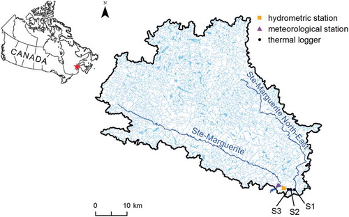
Water temperature, air temperature and flow data were recorded on the study sites from 2007 to 2013. The observed hourly data on the first and second variables are aggregated to daily averages. Figure 1 shows the location of the weather station (48°16ʹ37.2″N; 69°56ʹ2.399″W), the hydrometric station (48°16ʹ5.016″N; 69°54ʹ33.012″W) managed by the Ministry of Sustainable Development, Environment and the Fight against Climate Change (https://www.cehq.gouv.qc.ca/depot/historique_donnees/fichier/062803_Q.txt) and the thermistor S3 (107b temperature sensor, Campbell Scientific, ±0.5°C) (48°16ʹ20″N; 69°54ʹ50″W) used to measure water temperatures. For each year, only the measurements from May to October, which is the period corresponding to the ice-free season, were used in this study.

For all years, water temperature time series are incomplete (see Table 1) because of equipment malfunction or because of low water levels, which exposed the thermograph to the air.

Table 1. Number of concomitant records by year for the three variables: water temperature, air temperature and flow.

Year	Start of period (dd/mm)	End of period (dd/mm)	No. of observations
2005	23/06	25/07	33
2006	0	0	0
2007	04/07	01/10	89
2008	0	0	0
2009	28/07	08/09	43
2010	24/05	16/10	146
2011	01/05 27/07	17/07 31/10	175
2012	20/06	31/10	134
2013	12/06	31/10	141
2014	16/05 06/09	11/06 31/10	83
2015	01/05	19/07	80

3 Statistical methods

3.1 Generalized additive model

The generalized additive model (GAM) was introduced by Hastie and Tibshirani (1986). The GAM, which is an extension of the generalized linear model (GLM) (McCullagh and Nelder 1989), has many advantages over the latter model. Unlike the GLM, which is based on the strong assumption of linearity of the parameters, the GAM assumes no form of dependency and the relationship is not necessarily linear. Its principle is based on modelling the response using a sum of nonlinear functions, which allows one to model more precisely the influence of each explanatory variable. This specificity makes it a popular tool in modelling the effects of environmental variables because these effects are often nonlinear and are difficult to specify parametrically (Peng and Dominici 2008, Bruneau and Grégoire 2011). The literature review of Jbilou and El Adlouni (2012) presented the potential of the GAM in environmental health studies as a powerful technique to identify nonlinear relationships between an explanatory environmental variable and a health-dependent variable.

If restricted to the GLM, given a response variable y and p explanatory variables x₁, x₂, …, x_p, the GLM is written as:

(1) $g(\mathrm{E}(y))={\beta }_0+{\beta }_1{x}_1+{\beta }_2{x}_2+\cdots +{\beta }_p{x}_p+\epsilon$(1)

where g is the link function, which is a parametric function allowing for extension of the Gaussian distribution to the exponential family and which connects the average of the dependent variable to a set of explanatory variables; E(y) is the expected value of the response variable; and ε is the error assumed to be normally distributed with variance σ_ε.

In the case of standard linear regression, the link function g is the identity. The GAM still uses a link function g, as in the case of the GLM, but the linear dependency is replaced by more general dependency functions. This model is written as follows:

(2) $g(\mathrm{E}(y))={\beta }_0+f_1\left(x_1\right)+f_2\left(x_2\right)+...+f_p\left(x_p\right)+\epsilon$(2)

The implementation of this model requires the estimation of the smooth nonlinear functions f_i(x_i), i = 1, …, p, for each explanatory variable x_i.

To avoid the problem of overfitting, the penalized GAM was used (Wood 2006), where smoothing¹ functions f_i are cubic smoothing splines² (also referred to as penalized splines). These splines are defined as the solution to the following optimization problem: among the twice continuously differentiable functions, keeping only those minimizing the sum of the penalized squares, which is referred to as the penalized residual sum of squares:

(3) $\underset{f_i\in C^2}{argmin}({∥y-f_i(x_i)∥}^2+\sum _i{\lambda }_i\int f_i^{{\hspace{0.17em}}^{\prime \prime }}{(x)}^2\mathrm{d}x)$(3)

The first term of equation (3) measures the fit to data and the second term penalizes curvature in the function. Smoothing parameters ${\lambda }_1,...,{\lambda }_p$ represent the penalties on the roughness of the fitted function associated with each explanatory variable x. They control the smoothing level of each function f_i and the compromise between the bias and the variance. The underlying idea is to position far more nodes than deemed necessary and, by the use of a penalty, eliminate those nodes providing insufficient information.

The optimization problem (equation (3)) has a formulation parametric equivalent, based on the decomposition of the f_i functions using cubic splines (De Boor 1978). Given that b_j represents the cubic B-spline, each f_i function will have the following form:

(4) $f_i=B^i{\beta }^i\mathrm{w}\mathrm{h}\mathrm{e}\mathrm{r}\mathrm{e}B\beta ={\sum }_j{b}_j{\beta }_j$(4)

The optimization problem (equation (3)) becomes:

(5) $\arg \underset{({\beta }^1,\mathrm{...},{\beta }^p)\in {ℝ}^{k\times p}}{\min }\left({\Vert y-{\beta }_0+{\displaystyle \sum _{i=1}^p{B}^i{\beta }^i}\Vert }^2+{\displaystyle \sum _{i=1}^p{\lambda }_i}\int {\left\{(B^i{\beta }^i{)}^{″}\right\}}^2\text{d}x\right)$(5)

where f_i is the ith regression function in the additive model, f″ denotes the second derivative of f, || || is the Euclidean norm and ${\lambda }_1,...,{\lambda }_p$ are penalty terms.

The resolution of the problem (equation (5)) and the fit of the model are done using the iterative reweighted least squares algorithm (IRLS). The name of this algorithm comes from the fact that in each iteration the problem solved is equivalent to a weighted least squares problem.

The second derivative of the smoothing function f_i characterizes the form of the smoothing. A high value of f_i″ means that f_i is rough; however, a straight line has a second derivative equal to zero. For optimal values of λ_i the penalties should avoid the two extremes and allow a good fit with a balanced minimization of bias and variance. The choice of these parameters is done by using generalized cross-validation (GCV) and performance metrics.

The implementation of the GAM model was made with R software (Team 2014) provided with the package “mgcv” (minimizing generalized cross-validation; Wood 2013) version 1.7–22. This package uses a modified version of the GCV method by Wood (2006) to automatically determine the optimal smoothing associated with each explanatory variable. The threshold of the smoothing functions of explanatory variables to be retained is 5%.

The main objective of the regression is to investigate whether some of the short-term variation in the response variable can be explained by changes in the explanatory variables. These series often have long-term trend changes such as seasonal variations. These variations and seasonal trends are likely to dominate the data, which may make it more difficult to quantify the short-term associations between response variable and explanatory variables, and influence the interpretation of short-term response between series (Peng and Dominici 2008). As our interest is in short-term associations, the objective is to control these low-frequency changes in the model by including a term that is time dependent and capable of accounting for the periodicity in seasonal time series (Bhaskaran et al. 2013). In the GAM, the seasonality can be contolled by introducing a time-smoothing spline function.

3.2 Comparison with other models

The GAM described above was compared to three other popular models that are used to predict water temperature. These are the logistic, residuals regression and linear regression models.

3.2.1 Logistic model

This nonlinear regression model is based on the development of a logistic function (equation (6)) that has three parameters with physical significance (Mohseni et al. 1998). It allows water temperature to be modelled as a function of air temperature, and provides a better fit than a linear regression for the extreme values. This model has been extensively used with weekly data and some applications have been made at a daily time step (e.g. St-Hilaire et al. 2012).

(6) $T_{\mathrm{w}}=\frac{\alpha }{1+{\mathrm{e}}^{\gamma (\left(\beta -T_{\mathrm{a}}\right)}}$(6)

where T_w and T_a represent water and air temperatures; α is a coefficient that estimates the highest water temperature; β is the air temperature at the inflexion point; and γ represents the steepest slope of the logistic function. These parameters are estimated using a nonlinear regression approach minimizing the sum of square errors.

3.2.2 Residuals regression model

This approach consists of separating water and air temperature time series into two components: the long-term annual, or seasonal, component and the short-term component, or residuals:

(7) $T_{\mathrm{w}}={T_{\mathrm{w}\mathrm{A}}}_{(t)}+{{\mathrm{R}}_{\mathrm{w}}}_{(t)}$(7)

(8) $T_{\mathrm{a}}={T_{\mathrm{a}\mathrm{A}}}_{(t)}+{R_{\mathrm{a}}}_{(t)}$(8)

where T_wA(t) and T_aA(t) are the long-term annual components of water and air temperature, respectively; R_w(t) and R_a(t) are the short-term components of water and air temperature, respectively; and t represents Julian day or the day of year (e.g. 1 June = 152).

The seasonal component is modelled using a sinusoidal function for time series of both water and air temperatures (Cluis 1972):

(9) ${T_{\mathrm{w}\mathrm{A}}}_{(t)}=a_{\mathrm{w}}+b_{\mathrm{w}}sin\left[\frac{2\pi }{365}{(t+t_0}_{\mathrm{w}})\right]$(9)

(10) ${T_{\mathrm{a}\mathrm{A}}}_{(t)}=a_{\mathrm{a}}+b_{\mathrm{a}}sin\left[\frac{2\pi }{365}{(t+t_0}_{\mathrm{a}})\right]$(10)

where T_wA(t) and T_aA(t) are the seasonal components of a water temperature and air temperature time series; a_w, b_w, t_0w, a_a, b_a, t_0a are fitted coefficients that can be estimated using a nonlinear regression approach minimizing the sum of square errors.

The residual water temperatures (departures from the long-term water annual component) were modelled using a multiple regression with air temperature residuals (departures from the long-term air annual component) of lag 1 and 2 as input variables (Kothandaraman 1971). The residuals regression model is given by:

(11) ${R_{\mathrm{w}}}_{(t)}={\beta }_1{R_{\mathrm{a}}}_{(t-1)}+{\beta }_2{R_{\mathrm{a}}}_{(t-2)}+{\epsilon }_{(t)}$(11)

where R_w(t) is the residual water temperature at time t; $R_{a(t-1)}$and ${R_a}_{(t-2)}$ are the residuals of air temperature at times $t-1$ and $t-2$; β₁ and β₂ represent the regression coefficients estimated using the least squares method; and ε(t) is the error assumed to be normally distributed.

3.2.3 Linear regression model

The linear regression model (equation (12)) is based on the strong assumption of linearity of the parameters (Cornillon and Matzner-Lober 2007). It explains a response variable Y, assumed to follow a normal distribution, depending on the number of explanatory variables $X_1,\dots ,X_n$ and a normal error term ε of zero mean and variance σ²:

(12) $Y={\alpha }_0+{\alpha }_1{X}_1+\cdots +{\alpha }_n{X}_n+\epsilon$(12)

where ${\alpha }_1,{\alpha }_2,...,{\alpha }_n$ represent the regression coefficients estimated using the least squares method.

3.3 Model evaluation and validation

All models were validated by the technique of cross-validation (leave-one-out cross-validation year method or jack-knife technique; Quenouille 1949). This procedure consists of temporarily removing the data on water temperature for one year from the database and using the rest of the database for calibration. Then, the temperature values of the year removed are estimated. This operation is repeated for all years to find an estimate for all the water temperature values for comparison between the estimated values and the observed values using three criteria: the root mean square error (RMSE) (Janssen and Heuberger 1995), the bias error (B) and the Nash-Sutcliffe coefficient of efficiency (NSC) (Nash and Sutcliffe 1970), given by:

(13) $\mathrm{R}\mathrm{M}\mathrm{S}\mathrm{E}=\sqrt{\frac{1}{n}\sum _{i=1}^n{\left(P_i-O_i\right)}^2}$(13)

(14) $B=\frac{1}{n}\sum _{i=1}^n(P_i-O_i)$(14)

(15) $\mathrm{N}\mathrm{S}\mathrm{C}=1-\frac{{\sum }_{i=1}^n{\left(P_i-O_i\right)}^2}{{\sum }_{i=1}^n{\left(\bar{O}-O_i\right)}^2}$(15)

where n is the number of data points; P_i and O_i are the predicted and observed values of daily mean water temperature, respectively; and $\bar{O}$ is the mean of observed daily water temperature values.

4 Results

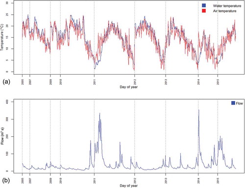
The daily averages were calculated from hourly water and air temperature data for the ice-free periods between 2005 and 2015, with no data available for 2006 and 2008. Within each year, we have observations for the period from May to October (184 days). The series are presented graphically in Fig. 2. Figure 2(a) shows that the amplitudes of variation of air temperature are more pronounced than those of water temperature. However, it should be noted that water temperature reached relatively high mean values (higher than mean air temperature values) during the summers of 2005, 2007, 2010, 2012 and 2013. This is not typical of most eastern Canadian rivers, but is often observed in wide, shallow water courses (Caissie 2006). Figure 2(b) suggests a nonlinear relationship between water temperature and the two explanatory variables: air temperature and flow rate.

Figure 2. (a) Average daily water and air temperatures from 2005 to 2015; and (b) average daily flows from 2005 to 2015.

4.1 GAM

A GAM was applied by incorporating air temperature and flow rate as variables affecting the thermal regime. The introduction of the day of the year variable in this model allowed us to reproduce the seasonality of the data.

After removing the other explanatory variables, the GAM allows the influence of a single explanatory variable on the response variable to be estimated. It produces a visual representation of the relationship between water temperature and air temperature or flow rate. The analytical results of this model show that the effects of air temperature, flow rate and seasonality are significantly nonlinear, with a critical probability (P value) of less than 0.00001 (see Table 2). This means that the nonlinear portion is not negligible and considering just the linear component of these effects is not enough. The deviance (see Table 2) explained by the model has a similar meaning as R² in the linear case. The calculation of deviance for a model is made with respect to the deviation of the null (non-explanatory) model. The percentage of the total variance explained by this model is 94.6% (see Table 2). The nonlinear net effects of air temperature, flow rate and seasonality are presented in Fig. 3. The shading corresponds to a confidence interval of 95%. The black dots, representing partial residuals, are the residuals that remain after removing the effect of all other predictors. The plot allows us to understand the nature of the relationship between air temperature or flow rate and water temperature. One can see that the cloud of the smooth curve of air temperature (Fig. 3(a)) lightly draws an S-shape. The flow rate represents a somewhat decreasing effect (Fig. 3(b)).

Table 2. Significance of effects.

Smoothing functions	Estimated degrees of freedom	Fisher test	P-value
S (air temperature)	3.6	242.9
S (flow)	8.0	43.4	2.2 × 10^−16
S (day of the year)	8.4	85.44
R^2_adj		0.94
Deviance explained		94.6%

Figure 3. Estimated smoothing functions representing the contributions of predictors: (a) air temperature; (b) flow; and (c) day of year.

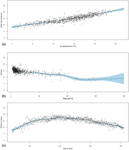
The effect of the flow rate is marked by the presence of spring floods. This effect is present in spring because of the large volume of water resulting from snowmelt. The air temperature effect is more pronounced during summer when the river has a low flow rate, which means that air temperature is closely associated with water temperature during this season. The inclusion of a flow and an air temperature implicitly takes into account the specificities of each season, while the inclusion of the Julian date minimizes the risk of increased error associated with the hysteresis effect.

The contribution of an explanatory variable to the deviance explained by the model is equal to the deviance of the full model minus the deviance of the reduced model of this explanatory variable divided by the deviance of the null model (Turgeon 2012). In terms of percentage, the contribution associated with each explanatory variable is relative to the sum of the contributions of all the explanatory variables included in the model. For the proposed GAM, the contributions to the deviance of the air temperature, flow rate and season are 50%, 17% and 38%, respectively. For this case study, the GAM gave a good fit of water temperature according to air temperature and flow rate, with an overall prediction error of 1.44°C. Thereafter, it was compared to three other popular models. Finally, residual analysis was conducted to determine whether the GAM can be accepted. This analysis was performed on the cross-validation residuals to avoid the data overfitting problem. Figures 4 and 5 confirm the normality of the distribution of these residuals. Furthermore, the graph of these residuals in terms of estimated water temperature shows a cloud of points that are uniformly dispersed and have an equal spread everywhere (Fig. 6). This indicates that no structure remains in the residuals.

Figure 4. Normal Q-Q plot of GAM residuals.

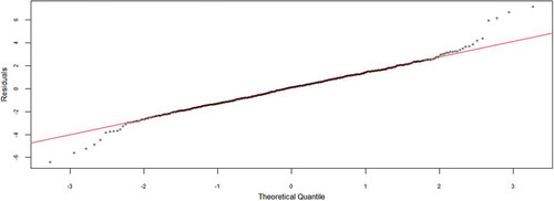
Figure 5. Normal distribution of GAM residuals.

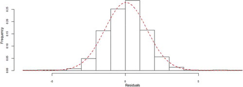
Figure 6. Residuals versus estimated water temperatures.

4.2 Logistic model

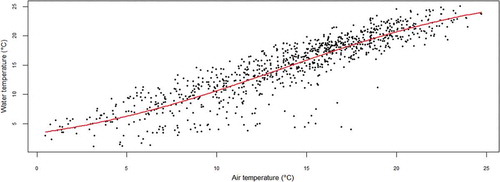
The logistic model (Mohseni et al. 1998), which connects water temperature to air temperature (equation (6)), was applied to the daily average of the water and air temperatures. The estimation of this logistic function is given by:

(15) $T_{\text{w}}=\frac{28.64}{1+{\text{e}}^{0.15(13.56-T_a})}$(15)

Water and air temperature daily means show strong dispersion (Fig. 7). The logistic function fits the general trend, but is not well suited for daily data, although it has been shown to perform well at the weekly time step (Benyahya et al. 2007). The total variability explained by this model is 80%. The overall prediction error (RMSE) is 2.56°C.

Figure 7. Relationship between daily mean water temperature and mean air temperature and a fitted logistic function.

4.3 Residuals regression model

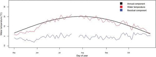
Initially, the long-term seasonal component of water and air temperatures was fitted with a sinusoidal function by applying equations (9) and (10). This explains 81.6% and 69% of the total variability of water and air temperatures, respectively. The highest daily average water temperature for the annual component is reached on 31 July (day 212 equivalent to t = 92) and is 20.15°C. In contrast, the highest daily average air temperature for the annual component is reached on 25 July (day 206 equivalent to t = 86) and is 18.30°C. For example, Fig. 8 shows the estimation of the water temperature components for 2011 using the following sinusoidal function:

(16) ${T_{\mathrm{w}\mathrm{A}}}_{(t)}=2.85+17.3sin\left[\frac{2\pi }{365}(t-0.86)\right]$(16)

Figure 8. Mean daily water temperature, annual component estimated by sinusoidal function and the residual component.

Once the annual component was removed from both air and water temperature time series, the water temperature residuals were estimated by a regression model, given by:

(17) ${R_w}_{(\mathrm{t})}=0.46{R_{\mathrm{a}}}_{(t-1)}+0.15{R_{\mathrm{a}}}_{(t-2)}+{\epsilon }_{(t)}$(17)

The coefficients of lag 1 and lag 2 for the air temperature residuals were significant in explaining the water temperature residuals, and the intercept was insignificant. This model is better than the logistic model for representing the daily data. The air temperature residuals of lag 1 and lag 2 explained 43.98% of the total variability of water temperature residuals. However, the total variability explained by this model when the annual component was added is 90.5% and the overall prediction error (RMSE) is 2°C.

4.4 Linear regression model

For our study, this simplest model was applied to relate the dependent variable, the daily average of water temperature T_w, to the explanatory variables, the daily average of air temperature T_a and flow F (Neumann et al. 2003). Using the least squares method, the following equation was obtained:

(18) $T_{\mathrm{w}}=4.26+0.86T_{\mathrm{a}}-0.04F$(18)

This linear model is better than the residuals regression model for representing the daily average water temperature. It explained 90% of the total variability of water temperature and the RMSE is 1.83°C.

4.5 Comparative study

The performance of all models, GAM, logistic, residuals and linear regression, was assessed using annual cross-validation and the three indices, RMSE, bias and NSC. These indices were calculated during the cross-validation for each year and for the entire period (see Table 3).

Table 3. Results of the cross-validation of water temperature (°C) modelling expressed by RMSE, bias error and NSC by the GAM, logistic, residuals regression and linear regression approaches.

Year	Model
	GAM			Multiple regression			Residuals regression			Logistic
	RMSE(°C)	Bias(°C)	NSC	RMSE(°C)	Bias(°C)	NSC	RMSE(°C)	Bias(°C)	NSC	RMSE(°C)	Bias(°C)	NSC
2005	1.72	−0.95	0.39	1.87	−1.2	0.27	2.31	−1.59	−0.1	1.97	−1.24	0.19
2007	1.2	0.24	0.87	1.42	−0.33	0.82	1.64	0.7	0.77	1.8	−1.1	0.71
2009	1.12	0.29	0.82	1.29	0.04	0.76	1.69	1.42	0.58	1.8	−0.12	0.52
2010	1.83	−0.68	0.86	1.74	−0.68	0.87	2.32	−1.12	0.77	2.07	−1.43	0.82
2011	1.54	0.29	0.93	2.26	0.33	0.85	2.47	1.15	0.83	3.37	1.68	0.67
2012	1.27	−0.17	0.95	1.63	0	0.92	1.27	−0.71	0.95	1.82	−0.7	0.9
2013	1.12	0.39	0.94	1.59	0.29	0.89	1.53	0.44	0.9	1.76	−0.23	0.86
2014	1.48	−0.1	0.97	2.07	0.12	0.93	2.51	−0.04	0.9	3.68	0.62	0.79
2015	1.38	−0.22	0.93	2.01	0.44	0.85	1.68	0.4	0.9	3.28	1.6	0.61
Global	1.44	−0.04	0.94	1.83	−0.02	0.9	2	0.11	0.88	2.56	−0.01	0.8
Range	1.12–1.83	−0.95 to 0.39	0.39–0.97	1.29–2.26	−1.2 to 0.44	0.27–0.93	1.27–2.51	−1.59 to 1.42	−0.1 to 0.95	1.76–3.68	−1.43 to 1.68	0.19–0.86

Overall, the GAM performs better than the other three models with a RMSE of 1.44°C between predicted and observed values. The logistic, the residuals regression and the linear models have an overall RMSE of 2.56°C, 2.0°C and 1.83°C, respectively. These three models performed less well than the GAM, but the linear model is better than the other two traditional approaches. The annual values of RMSE vary between 1.12°C and 1.83°C for the GAM model, between 1.76°C and 3.68°C for the logistic model, between 1.27°C and 2.51°C for the residuals regression model and between 1.29°C and 2.26°C for the linear model. The overall bias is very low and centred at zero, but the range is wide for the logistic and the residuals models (i.e. −0.95–0.39°C for GAM, −1.43–1.68°C for the logistic model, −1.59–1.42°C for the residuals regression model and −1.29–0.44°C for the linear model).

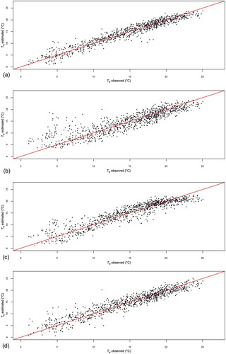
The NSC criterion indicates a good match of GAM model output to observed data, with a value of 0.94. This result is confirmed by the graphical presentation (see Fig. 9(a)) of estimated values versus the observed values. Figure 9(a) shows an alignment concentrated around the first bisector, and indicates that the gap between the observed values and the values predicted by the GAM is less than with the other three models. The adequacy of the logistic model for this case study is barely acceptable. The residuals regression results were also generally better than those of the logistic model, but not as good as the GAM results. However, the linear model is more suitable in comparison with the logistic model and the residuals regression model. The NSC is 0.80 for the logistic model, 0.88 for the residuals regression model and 0.90 for the linear model. Figure 9(b) shows the values estimated by the logistic model versus the observed values, showing that this model overestimates the low values of water temperature and has strong dispersion. Figure 9(c) demonstrates that the residuals regression model underestimates the highest values and overestimates the low values of water temperature. This model does not account for the flow rate, so the overestimations of water temperature were generally observed in spring at higher water levels, while the underestimations were observed during summer, when water levels are lower. Nevertheless, Fig. 9(d) shows dispersion of the values around the first bisector that is more pronounced for the linear model than for the GAM.

Figure 9. Scatterplot of observed versus predicted values for (a) the GAM model; (b) the logistic model; (c) the residuals regression model; and (d) the linear regression model for the season of May–October (2005–2015).

5 Discussion and conclusions

The assessment described in this paper will help to determine whether the GAM is a promising tool that can help in the management of aquatic resources by providing accurate temperature simulations/predictions. The performance of the GAM was compared to the logistic, residuals regression and linear models. The logistic model performed poorly for daily data (RMSE = 2.56°C). This is consistent with the results of Caissie et al. (2001) on the maximum daily water temperature. Indeed, this model is more suited for longer time steps, such as weekly data (Benyahya et al. 2007), for which it has been widely used. The residuals regression model, which separates the water and air temperature times series into two components—a seasonal component and a residual component—also had relatively acceptable performance (RMSE = 2.00°C). Better performance was obtained with this type of model in previous studies, such as that of Caissie et al. (1998). This model does not take into account the autocorrelation in the water temperature time series, which is usually significant (Caissie et al. 1998). The effect of the flow on water temperature is also excluded from this model, as in the case of the logistic method. It should also be noted that the period of this study contains three years with relatively warm water temperatures, which is atypical for the Sainte-Marguerite River (see Guillemette et al. 2009 for monthly maxima). Those limitations have affected the performance of the residuals regression approach for this river. Moreover, the strong correlation between lag 1 and lag 2 of the air temperature residuals causes a multicollinearity problem for this regression; thus, the results may be less accurate. The linear model can take into account the effect of the flow, which explains the better results obtained when compared to the logistic and the residuals regression models. However, this model takes into consideration just the linear effects, while our dataset shows the existence of a nonlinear relationship between water temperature and air temperature, as well as between water temperature and flow.

The results of the GAM model showed that it was very flexible in adjusting nonlinear relationships between water temperature and the explanatory variables (air temperature and flow), especially for atypical data as in this study. On an annual basis, this model gave a high RMSE for two of the nine years of study. The first year for which the RMSE was relatively high is 2009 (RMSE = 1.72°C). For this year, we adjusted the GAM only for the warmer months due to missing data. Obtaining this RMSE is justified by the data missing during the cold period. The second year with weaker performance of the GAM is 2010. This was the warmest year in the time series used in this study and differs from other years by the presence of the lowest precipitation of the study period. The flow remained constant over most of the spring and autumn periods of 2010, which reduced the effect of the flow variability on the water temperature for this year. The flow rate effect is marked by the presence of flooding, but this is weak during the warm period when the air temperature effect dominates. The inclusion of flow implicitly allowed the specificities of each season to be reflected. The residual analysis of the GAM gives confidence in its use. Its relative ease of implementation and adaptation could make it an ideal option for forecasting water temperature, given discharge and air temperature short-term forecasts. To sum up, the GAM model established very flexible nonlinear relationships between water temperature and the explanatory variables, air temperature and flow. It gave a better fit for the water temperature data of the Sainte-Marguerite River and, in particular, it was more robust in the case of atypical data. To validate the preliminary findings of this study, application on other sites with no atypical data would be useful. Validation on other sites would allow us to judge whether it can be used as a potential tool for effective management of aquatic systems. It could then be used to predict the impact of climate change on river temperature and to mitigate its effects on fish habitats.

Disclosure statement

No potential conflict of interest was reported by the authors.

Additional information

Funding

The financial support of the Natural Sciences and Engineering Research Council of Canada is acknowledged.

Notes

¹ A smoothing is a non-parametric tool that controls the regularity of a function (regression or density). Regularity is controlled by the degree of differentiability of the function.

² A cubic spline is a polynomial function of degree 3 (or about 4) piecewise and breaking points called nodes. It is C4-2 class at each node.

References

- Acuña, V. and Tockner, K., 2009. Surface–subsurface water exchange rates along alluvial river reaches control the thermal patterns in an Alpine river network. Freshwater Biology, 54, 306–320. doi:10.1111/fwb.2009.54.issue-2
- Ahmadi-Nedushan, B., et al., 2007. Predicting river water temperatures using stochastic models: case study of the Moisie River (Quebec, Canada). Hydrological Processes, 21 (1), 21–34. doi:10.1002/(ISSN)1099-1085
- Arismendi, I., et al., 2012. The paradox of cooling streams in a warming world: regional climate trends do not parallel variable local trends in stream temperature in the Pacific continental United States. Geophysical Research Letters, 39 (10), L104901. doi:10.1029/2012GL051448
- Baird, O.E. and Krueger, C.C., 2003. Behavioral thermoregulation of brook and rainbow trout: comparison of summer habitat use in an Adirondack River, New York. Transactions of the American Fisheries Society, 132 (6), 1194–1206. doi:10.1577/T02-127
- Bélanger, M., et al., 2005. Estimation de la température de l’eau de rivière en utilisant les réseaux de neurones et la régression linéaire multiple. Revue des sciences de l’eau/Journal of Water Science, 18 (3), 403–421.
- Benyahya, L., et al., 2007. A review of statistical water temperature models. Canadian Water Resources Journal, 32 (3), 179–192. doi:10.4296/cwrj3203179
- Benyahya, L., et al., 2008. Comparison of non-parametric and parametric water temperature models on the Nivelle River, France. Hydrological Sciences Journal, 53 (3), 640–655. doi:10.1623/hysj.53.3.640
- Bhaskaran, K., et al., 2013. Time series regression studies in environmental epidemiology. International Journal of Epidemiology, 42 (4), 1187–1195. doi:10.1093/ije/dyt092
- Bruneau, B. and Grégoire, F., 2011. Étude de la distribution spatiale des données d’abondance de maquereau bleu (Scomber scombrus) et de capelan (Mallotus villosus) des relevés d’hiver aux poissons de fond des Divisions 4VW de l’OPANO à l’aide de modèles additifs généralisés. Rapport technique canadien des sciences halieutiques et aquatiques, 2930, vi + 22.
- Cairns, J.J., et al., 1978. Effects of temperature on aquatic organism sensitivity to selected chemicals. In: Bulletin 106. Virginia Water Resources Center. 92.
- Caissie, D., 2006. The thermal regime of rivers: a review. Freshwater Biology, 51 (8), 1389–1406. doi:10.1111/fwb.2006.51.issue-8
- Caissie, D., El-Jabi, N., and Satish, M.G., 2001. Modelling of maximum daily water temperatures in a small stream using air temperatures. Journal of Hydrology, 251 (1–2), 14–28. doi:10.1016/S0022-1694(01)00427-9
- Caissie, D., El-Jabi, N., and St-Hilaire, A., 1998. Stochastic modelling of water temperatures in a small stream using air to water relations. Canadian Journal of Civil Engineering, 25 (2), 250–260. doi:10.1139/l97-091
- Caissie, D., Satish, M.G., and El-Jabi, N., 2007. Predicting water temperatures using a deterministic model: application on Miramichi River catchments (New Brunswick, Canada). Journal of Hydrology, 336 (3–4), 303–315. doi:10.1016/j.jhydrol.2007.01.008
- Caldwell, J., Rajagopalan, B., and Danner, E., 2014. Statistical modelling of daily water temperature attributes on the Sacramento River. Journal of Hydrologic Engineering, 20 (5), 1–10.
- Chenard, J.-F. and Caissie, D., 2008. Stream temperature modelling using artificial neural networks: application on Catamaran Brook, New Brunswick, Canada. Hydrological Processes, 22 (17), 3361–3372. doi:10.1002/hyp.v22:17
- Cluis, D.A., 1972. Relationship between stream water temperature and ambient air temperature. Nordic Hydrology, 3 (2), 65–71.
- Cole, J.C., et al., 2014. Developing and testing temperature models for regulated systems: A case study on the Upper Delaware River. Journal of Hydrology, 519, 588–598. doi:10.1016/j.jhydrol.2014.07.058
- Connor, W.P., Piston, C.E., and Garcia, A.P., 2003. Temperature during incubation as one factor affecting the distribution of Snake River fall Chinook salmon spawning areas. Transactions of the American Fisheries Society, 132 (6), 1236–1243. doi:10.1577/T02-159
- Cornillon, P.-A. and Matzner-Lober, E., 2007. Régression: théorie et applications. Paris: Springer.
- Cox, M.M. and Bolte, J.P., 2007. A spatially explicit network-based model for estimating stream temperature distribution. Environmental Modelling & Software, 22 (4), 502–514. doi:10.1016/j.envsoft.2006.02.011
- Crozier, L.G. and Zabel, R.W., 2006. Climate impacts at multiple scales: evidence for differential population responses in juvenile Chinook salmon. Journal of Animal Ecology, 75 (5), 1100–1109. doi:10.1111/j.1365-2656.2006.01130.x
- Daigle, A., Jeong, D.I., and Lapointe, M.F., 2014. Climate change and resilience of tributary thermal refugia for salmonids in eastern Canadian rivers. Hydrological Sciences Journal, 1–20. doi:10.1080/02626667.2014.898121
- De Boor, C., 1978. A practical guide to splines. Paris: Springer Verlag.
- Demars, B.E.N.O.Î.T.O.L., et al., 2011. Temperature and the metabolic balance of streams. Freshwater Biology, 56 (6), 1106–1121. doi:10.1111/fwb.2011.56.issue-6
- DeWeber, J.T. and Wagner, T., 2014. A regional neural network ensemble for predicting mean daily river water temperature. Journal of Hydrology, 517, 187–200. doi:10.1016/j.jhydrol.2014.05.035
- Ducharne, A., 2008. Importance of stream temperature to climate change impact on water quality. Hydrology and Earth System Sciences Discussions, 12 (3), 797–810. doi:10.5194/hess-12-797-2008
- Dugdale, S.J., Bergeron, N.E., and St-Hilaire, A., 2013. Temporal variability of thermal refuges and water temperature patterns in an Atlantic salmon river. Remote Sensing of Environment, 136, 358–373. doi:10.1016/j.rse.2013.05.018
- Eaton, J., et al., 1995. A field information-based system for estimating fish temperature tolerances. Fisheries, 20 (4), 10–18. doi:10.1577/1548-8446(1995)020<0010:AFISFE>2.0.CO;2
- Eaton, J.G. and Scheller, R.M., 1996. Effects of climate warming on fish thermal habitat in streams of the United States. Limnology and Oceanography, 41 (5), 1109–1115. doi:10.4319/lo.1996.41.5.1109
- Ebersole, J.L., Liss, W.J., and Frissell, C.A., 2003. Thermal heterogeneity, stream channel morphology, and salmonid abundance in northeastern Oregon streams. Canadian Journal of Fisheries and Aquatic Sciences, 60 (10), 1266–1280. doi:10.1139/f03-107
- Edinger, J.E., Duttweiler, D.W., and Geyer, J.C., 1968. The response of water temperatures to meteorological conditions. Water Resources Research, 4 (5), 1137–1143. doi:10.1029/WR004i005p01137
- Edwards, P.A. and Cunjak, R.A., 2007. Influence of water temperature and streambed stability on the abundance and distribution of slimy sculpin (Cottus cognatus). Environmental Biology of Fishes, 80 (1), 9–22. doi:10.1007/s10641-006-9102-8
- Elliott, J. and Hurley, M., 1997. A functional model for maximum growth of Atlantic salmon parr, Salmo salar, from two populations in northwest England. Functional Ecology, 11 (5), 592–603. doi:10.1046/j.1365-2435.1997.00130.x
- Erickson, T.R. and Stefan, H.G., 2000. Linear air/water temperature correlations for streams during open water periods. Journal of Hydrologic Engineering, 5 (3), 317–321. doi:10.1061/(ASCE)1084-0699(2000)5:3(317)
- Ferrari, M.R., Miller, J.R., and Russell, G.L., 2007. Modeling changes in summer temperature of the Fraser River during the next century. Journal of Hydrology, 342 (3–4), 336–346. doi:10.1016/j.jhydrol.2007.06.002
- Ficke, A.D., Myrick, C.A., and Hansen, L.J., 2007. Potential impacts of global climate change on freshwater fisheries. Reviews in Fish Biology and Fisheries, 17 (4), 581–613. doi:10.1007/s11160-007-9059-5
- Ficklin, D.L., Stewart, I.T., and Maurer, E.P., 2013. Effects of climate change on stream temperature, dissolved oxygen, and sediment concentration in the Sierra Nevada in California. Water Resources Research, 49 (5), 2765–2782. doi:10.1002/wrcr.20248
- Gras, R., 1969. Simulation du comportement thermique d’une rivière à partir des données fournies par un réseau classique d’observations météorologiques. Proceedings of the International Association of Hydraulic Research, Kyoto, 1, 491–502.
- Grégoire, Y. and Trencia, G., 2007. Influence de l’ombrage produit par la végétation riveraine sur la température de l’eau: un paramètre d’importance pour le maintien d’un habitat de qualité pour le poisson. Ministère des Ressources Naturelles et de la Faune, Secteur Faune Québec. Direction de l’aménagement de la faune de la région de la Chaudière-Appalaches.).
- Guay, J., et al., 2000. Development and validation of numerical habitat models for juveniles of Atlantic salmon (Salmo salar). Canadian Journal of Fisheries and Aquatic Sciences, 57 (10), 2065–2075. doi:10.1139/f00-162
- Guillemette, N., et al., 2009. Feasibility study of a geostatistical modelling of monthly maximum stream temperatures in a multivariate space. Journal of Hydrology, 364 (1–2), 1–12. doi:10.1016/j.jhydrol.2008.10.002
- Hari, R.E., et al., 2006. Consequences of climatic change for water temperature and brown trout populations in Alpine rivers and streams. Global Change Biology, 12 (1), 10–26. doi:10.1111/gcb.2006.12.issue-1
- Hastie, T. and Tibshirani, R., 1986. Generalized additive models. Statistical Science, 1, 297–310. doi:10.1214/ss/1177013604
- Isaak, D., et al., 2012. Climate change effects on stream and river temperatures across the northwest US from 1980–2009 and implications for salmonid fishes. Climatic Change, 113 (2), 499–524. doi:10.1007/s10584-011-0326-z
- Janssen, P. and Heuberger, P., 1995. Calibration of process-oriented models. Ecological Modelling, 83 (1–2), 55–66. doi:10.1016/0304-3800(95)00084-9
- Jbilou, J. and El Adlouni, S., 2012. Generalized Additive Models in Environmental Health: A Literature Review, Novel Approaches and Their Applications in Risk Assessment, Dr. Yuzhou Luo (Ed.), InTech. doi:10.5772/38811. Available from: http://www.intechopen.com/books/novel-approaches-and-their-applications-in-risk-assessment/generalized-additive-models-in-environmental-health-a-review-of-litterature
- Kaushal, S.S., et al., 2010. Rising stream and river temperatures in the United States. Frontiers in Ecology and the Environment, 8 (9), 461–466. doi:10.1890/090037
- Kothandaraman, V., 1971. Analysis of water temperature variations in large river. Journal of the Sanitary Engineering Division, 97 (1), 19–31.
- Lowney, C.L., 2000. Stream temperature variation in regulated rivers: evidence for a spatial pattern in daily minimum and maximum magnitudes. Water Resources Research, 36 (10), 2947–2955. doi:10.1029/2000WR900142
- Magnuson, J.J., Crowder, L.B., and Medvick, P.A., 1979. Temperature as an ecological resource. American Zoologist, 19 (1), 331–343. doi:10.1093/icb/19.1.331
- Marceau, P., Cluis, D., and Morin, G., 1986. Comparaison des performances relatives a un modèle déterministe et a un modèle stochastique de température de l’eau en rivière. Canadian Journal of Civil Engineering, 13, 352–364.
- Marszelewski, W. and Pius, B., 2015. Long-term changes in temperature of river waters in the transitional zone of the temperate climate: a case study of Polish rivers. Hydrological Sciences Journal, 61 (8), 182–187.
- McCullagh, P. and Nelder, J.A., 1989. Generalized linear models. London: CRC press.
- Moatar, F. and Gailhard, J., 2006. Water temperature behaviour in the River Loire since 1976 and 1881. Comptes Rendus Geoscience, 338 (5), 319–328. doi:10.1016/j.crte.2006.02.011
- Mohseni, O., Erickson, T.R., and Stefan, H.G., 1999. Sensitivity of stream temperatures in the United States to air temperatures projected under a global warming scenario. Water Resources Research, 35 (12), 3723–3733. doi:10.1029/1999WR900193
- Mohseni, O. and Stefan, H., 1999. Stream temperature/air temperature relationship: a physical interpretation. Journal of Hydrology, 218 (3–4), 128–141. doi:10.1016/S0022-1694(99)00034-7
- Mohseni, O., Stefan, H.G., and Eaton, J.G., 2003. Global warming and potential changes in fish habitat in US streams. Climatic Change, 59 (3), 389–409. doi:10.1023/A:1024847723344
- Mohseni, O., Stefan, H.G., and Erickson, T.R., 1998. A nonlinear regression model for weekly stream temperatures. Water Resources Research, 34 (10), 2685–2692. doi:10.1029/98WR01877
- Moore, R.D., 2006. Stream temperature patterns in British Columbia, Canada, based on routine spot measurements. Canadian Water Resources Journal, 31 (1), 41–56. doi:10.4296/cwrj3101041
- Morrill, J.C., Bales, R.C., and Conklin, M.H., 2005. Estimating stream temperature from air temperature: implications for future water quality. Journal of Environmental Engineering, 131 (1), 139–146. doi:10.1061/(ASCE)0733-9372(2005)131:1(139)
- Nash, J. and Sutcliffe, J.V., 1970. River flow forecasting through conceptual models part I—A discussion of principles. Journal of Hydrology, 10 (3), 282–290. doi:10.1016/0022-1694(70)90255-6
- Nelson, K.C. and Palmer, M.A., 2007. Stream temperature surges under urbanization and climate change: data, models, and responses. Journal of the American Water Resources Association (JWARA), 43 (2), 440–452. doi:10.1111/jawr.2007.43.issue-2
- Neuheimer, A.B. and Taggart, C.T., 2007. The growing degree-day and fish size-at-age: the overlooked metric. Canadian Journal of Fisheries and Aquatic Sciences, 64 (2), 375–385. doi:10.1139/f07-003
- Neumann, D.W., Rajagopalan, B., and Zagona, E.A., 2003. Regression model for daily maximum stream temperature. Journal of Environmental Engineering, 129 (7), 667–674. doi:10.1061/(ASCE)0733-9372(2003)129:7(667)
- Nohair, M., St-Hilaire, A., and Ouarda, T.B.M.J., 2008. Utilisation des réseaux de neurones et de la régularisation bayésienne en modélisation de la température de l’eau en rivière. Revue des sciences de l’eau/Journal of Water Science, 21 (3), 373–382.
- Olden, J.D. and Naiman, R.J., 2010. Incorporating thermal regimes into environmental flows assessments: modifying dam operations to restore freshwater ecosystem integrity. Freshwater Biology, 55 (1), 86–107. doi:10.1111/fwb.2009.55.issue-1
- Ozaki, N., et al., 2003. Statistical analyses on the effects of air temperature fluctuations on river water qualities. Hydrological Processes, 17 (14), 2837–2853. doi:10.1002/(ISSN)1099-1085
- Parmesan, C. and Yohe, G., 2003. A globally coherent fingerprint of climate change impacts across natural systems. Nature, 421 (6918), 37–42. doi:10.1038/nature01286
- Peng, R.D. and Dominici, F., 2008. Statistical methods for environmental epidemiology with R. R: A Case Study in Air Pollution and Health (Springer). doi:10.1007/978-0-387-78167-9
- Pike, A., et al., 2013. Forecasting river temperatures in real time using a stochastic dynamics approach. Water Resources Research, 49 (9), 5168–5182. doi:10.1002/wrcr.20389
- Pilgrim, J.M., Fang, X., and Stefan, H.G., 1998. Stream temperature correlations with air temperatures in Minnesota: implications for climate warming. JAWRA Journal of the American Water Resources Association, 34 (5), 1109–1121. doi:10.1111/jawr.1998.34.issue-5
- Prats, J., et al., 2012. Water temperature modeling in the Lower Ebro River (Spain): Heat fluxes, equilibrium temperature, and magnitude of alteration caused by reservoirs and thermal effluent. Water Resources Research, 48 (5), W05523. doi:10.1029/2011WR010379
- Quenouille, M.H., 1949. Approximate tests of correlation in time-series 3. Mathematical Proceedings of the Cambridge Philosophical Society, 45 (3), 483–484.
- Quigley, J.T. and Hinch, S.G., 2006. Effects of rapid experimental temperature increases on acute physiological stress and behaviour of stream dwelling juvenile chinook salmon. Journal of Thermal Biology, 31 (5), 429–441. doi:10.1016/j.jtherbio.2006.02.003
- Rabi, A., Hadzima-Nyarko, M., and Šperac, M., 2015. Modelling river temperature from air temperature: case of the River Drava (Croatia). Hydrological Sciences Journal, 60 (9), 1490–1507. doi:10.1080/02626667.2014.914215
- Risley, J.C., Roehl, E.A., and Conrads, P.A., 2003. Estimating watertemperatures in small streamsin western oregon using neural network models. in U.S. GEOLOGICAL SURVEY, Water-Resources Investigations Report 02-4218. Portland.
- Secondat, M., 1952. Les variations de la température et de la concentration en oxygène dissous des eaux lacustres et des eaux courantes. Leur retentissement sur la distribution des poissons. Bulletin Français de Pisciculture, 167, 52–59. doi:10.1051/kmae:1952001
- Segura, C., et al., 2015. A model to predict stream water temperature across the conterminous USA. Hydrological Processes, 29 (9), 2178–2195. doi:10.1002/hyp.v29.9
- Sharma, S., Walker, S.C., and Jackson, D.A., 2008. Empirical modelling of lake water‐temperature relationships: a comparison of approaches. Freshwater Biology, 53 (5), 897–911. doi:10.1111/j.1365-2427.2008.01943.x
- Smith, K., 1981. The prediction of river water temperatures/Prédiction des températures des eaux de rivière. Hydrological Sciences Bulletin, 26 (1), 19–32. doi:10.1080/02626668109490859
- Stefan, H.G. and Preud’homme, E.B., 1993. Stream temperature estimation from air temperature. JAWRA Journal of the American Water Resources Association, 29 (1), 27–45. doi:10.1111/jawr.1993.29.issue-1
- Stevens, H.H., Ficke, J.F., and Smoot, G.F., 1975. Water temperature-influential factors, field measurement, and data presentation. Washington: US Government Printing Office.
- St-Hilaire, A., et al., 2000. Water temperature modelling in a small forested stream: implication of forest canopy and soil temperature. Canadian Journal of Civil Engineering, 27 (6), 1095–1108. doi:10.1139/l00-021
- St-Hilaire, A., et al., 2012. Daily river water temperature forecast model with a k-nearest neighbour approach. Hydrological Processes, 26 (9), 1302–1310. doi:10.1002/hyp.8216
- Team, R.C., 2014. R: A language and environment for statistical computing. Vienna: R Foundation for Statistical Computing, 2012. (ISBN 3-900051-07-0).
- Turgeon, S., 2012. Modélisation de l’utilisation de l’habitat du béluga du Saint-Laurent en fonction de ses proies à l’embouchure de la rivière Saguenay et à la baie Sainte-Marguerite. Mémoire de maîtrise, Université de Montréal en vue de l’obtention du grade de Maître ès sciences (M.Sc.) en Géographie.
- Van Vliet, M., et al., 2011. Global river temperatures and sensitivity to atmospheric warming and changes in river flow. Water Resources Research, 47 (2), W02544. doi:10.1029/2010WR009198
- Vannote, R.L., et al., 1980. The river continuum concept. Canadian Journal of Fisheries and Aquatic Sciences, 37 (1), 130–137. doi:10.1139/f80-017
- Walther, G.-R., et al., 2002. Ecological responses to recent climate change. Nature, 416 (6879), 389–395. doi:10.1038/416389a
- Webb, B., 1996. Trends in stream and river temperature. Hydrological Processes, 10 (2), 205–226. doi:10.1002/(ISSN)1099-1085
- Webb, B., et al., 2004. Changing UK river temperatures and their impact on fish populations. In: Hydrology: science and practice for the 21st century, Volume II. Proceedings of the British Hydrological Society International Conference, Imperial College, July. London: British Hydrological Society, 177–191.
- Webb, B.W., Clack, P.D., and Walling, D.E., 2003. Water–air temperature relationships in a Devon river system and the role of flow. Hydrological Processes, 17 (15), 3069–3084. doi:10.1002/(ISSN)1099-1085
- Webb, B.W., et al., 2008. Recent advances in stream and river temperature research. Hydrological Processes, 22 (7), 902–918. doi:10.1002/(ISSN)1099-1085
- Wehrly, K.E., Brenden, T.O., and Wang, L., 2009. A comparison of statistical approaches for predicting stream temperatures across heterogeneous landscapes. JAWRA Journal of the American Water Resources Association, 45 (4), 986–997. doi:10.1111/jawr.2009.45.issue-4
- Wood, S., 2006. Generalized additive models: an introduction with R. Boca Raton, FL: CRC press.
- Wood, S., 2013. mgcv: mixed GAM computation vehicle with GCV/AIC/REML smoothness estimation. R package version 1.7-22.