Influence of spatial distribution of sensors and observation accuracy on the assimilation of distributed streamflow data in hydrological modelling

ABSTRACT

The aim of this study is to assess the influence of sensor locations and varying observation accuracy on the assimilation of distributed streamflow observations, also taking into account different structures of semi-distributed hydrological models. An ensemble Kalman filter is used to update a semi-distributed hydrological model as a response to measured streamflow. Various scenarios of sensor locations and observation accuracy are introduced. The methodology is tested on the Brue basin during five flood events. The results of this work demonstrate that the assimilation of streamflow observations at interior points of the basin can improve the hydrological models according to the particular location of the sensors and hydrological model structure. It is also found that appropriate definition of the observation accuracy can affect model performance and consequent flood forecasting. These findings can be used as criteria to develop methods for streamflow monitoring network design.

KEYWORDS:

• Flood forecasting
• data assimilation
• sensor location
• observation accuracy
• hydrological modelling

Editor M.C. Acreman; Associate editor G. Di Baldassarre

1 Introduction

Water system models of different types and complexity are used in flood early warning systems to predict floods and reduce their impact on urbanized areas (Todini et al. 2005). Since each model is a mathematical schematization of some natural physical process, a proper definition of the model structure and parameters is necessary in order to correctly represent the behaviour of the catchment and reduce model uncertainty (Pappenberger et al. 2006, Di Baldassarre and Montanari 2009). In addition, even in the case of perfect model structure and parameter estimation, an uncertain and inadequate characterization of rainfall inputs can produce imprecise runoff predictions (Beven 2004). A growing number of studies have analysed the impact of rainfall uncertainty on flood event prediction (Kavetski et al. 2006, Bárdossy and Das 2008, Moulin et al. 2009, McMillan et al. 2011).

Model updating techniques in hydrology are becoming an important tool for integrating the real-time observations of physical variables into water system models and thus reducing uncertainty in flood prediction (Liu et al. 2012). Hydrological observations, used to update the water models, can include streamflow (Pauwels and De Lannoy 2006, 2009, Weerts and El Serafy 2006), snow cover (Andreadis and Lettenmaier 2006), soil moisture (Brocca et al. 2010, 2012) or water level observations from in situ sensors (Madsen and Skotner 2005, Neal et al. 2007) and remote sensing (Giustarini et al. 2011).

Among model updating techniques, the methods used most in hydrology are divided into sequential and variational data assimilation (DA) methods (Liu and Gupta 2007). Any DA technique attempts to find the best new estimate of a system state on the basis of the (noisy) observations (McLaughlin 1995, 2002). Over recent decades, various DA approaches with differing complexity have been proposed.

For example, in direct insertion methods the observations are used to directly replace the model states since they are assumed to be more reliable than the model itself (Walker et al. 2001). In nudging techniques an additional term related to the reliability of the observations and model is used to update the model states (Houser et al. 1998).

The Kalman filter (KF) is one of the most commonly used DA methods. This is a mathematical tool that allows the assimilation, in an efficient recursive way, of observed noisy data into a linear dynamic system in order to update model states and thus improve model predictions (Kalman 1960). Variants of the Kalman filter for nonlinear systems, such as the extended Kalman filter (EKF) (Aubert et al. 2003), the ensemble Kalman filter (EnKF) (Reichle 2000, Evensen 2003, Komma et al. 2008, Mendoza et al. 2012, Rakovec et al. 2012) and the recursive ensemble Kalman filter (McMillan et al. 2013), have been proposed and applied in hydrology. Madsen and Cañizares (1999) compared the performance of the EKF and the EnKF in coastal area modelling. Their study showed that the EnKF did not fail in the case of strong nonlinear dynamics; however, it was very time consuming. Application of Kalman filtering methods to hydrodynamic modelling was explored by Verlaan and Heemink (1996), Verlaan (1998) and Cañizares (1999).

Yet another version of a nonlinear filter is the particle filter (PF) (Arulampalam et al. 2002) and this has also been used in flood forecasting tasks (Moradkhani et al. 2005, Salamon and Feyen 2009, Noh et al. 2014). In the PF, the posterior density function is represented by a set of random samples with associated weights according to the full prior density and resampling approach used (e.g. Arulampalam et al. 2002, Weerts and El Serafy 2006). The computational requirements, much higher than those of the KF, and problems with nearly noise-free models are seen as the main disadvantages of the PF.

In contrast to the previous sequential methods, variational assimilation methods have been widely used in weather forecasting and coastal engineering applications (Li and Navon 2001, Seo et al. 2003, 2009, Valstar et al. 2004, Fischer et al. 2005, Lorenc and Rawlins 2005, Lee et al. 2011, 2012, Liu et al. 2012). In these methods, a cost function that measures the difference between the error in initial conditions and the error between model predictions and observations over time is minimized to identify the best estimate of the initial state conditions (Seo et al. 2009, Lee et al. 2011).

The above-mentioned DA methods require significant real-time data on hydrological variables in order to update model states and subsequent flood forecasts. Nowadays, physical sensors of water level are increasingly available and in use by river basin authorities. However, it is important to assess the influence of sensor locations on the results of DA procedures since location affects hydrological model performance. Blöschl et al. (2008) proposed streamflow assimilation in a grid-based operational flood forecasting system; however, they did not analyse the effect of varying distributed streamflow observations within the river basin. Recently, authors have assessed the effect of interior discharge gauges on hydrological forecasts. In particular, Lee et al. (2011) assimilated streamflow and in situ soil moisture observations in a distributed hydrological model, showing that integration of streamflow observations at interior locations, in addition to those at the outlet, improves soil moisture and streamflow prediction along the channel network. Xie and Zhang (2010) and Chen et al. (2012) investigated the performance of a distributed model in the case of assimilation of distributed streamflow observations, concluding that the assimilation of runoff observations can significantly update the model states and parameters. Rakovec et al. (2012) analysed the sensitivity of EnKF to the updating frequency and number of distributed discharge gauges using a grid-based distributed hydrological model. They pointed out how hydrological forecasts can be improved by assimilating streamflow observations at interior points of the basin. However, analysis of the effect of sensor location on the DA performance is limited. Lee et al. (2012) considered various fixed spatiotemporal adjustment scales to update different spatial distributions of model states using a variational assimilation method. They demonstrated the sensitivity of model results to the spatial distribution of sensors. Mendoza et al. (2012) evaluated the performance of a distributed hydrological model in the case of assimilation of streamflow observations in a sparsely monitored catchment and pointed out that the upper basin contains the major source of uncertainty in hydrological process representation.

In addition to the impact of sensor locations on DA performance, another issue is the correct evaluation of the uncertainty affecting streamflow measurements (observation accuracy). In such observations, errors can be related to inappropriate water level (WL) measurement, or to the wrong assessment of the rating curve used to transform values of WL into discharges (Clark et al. 2008). Di Baldassarre and Montanari (2009) proposed a procedure for quantifying uncertainty of streamflow data, with particular focus on the analysis of rating curve uncertainty, neglecting however the uncertainty in the water level measurements. They found that estimation of river discharge using the rating curve method is affected by an overall error, at the 95% confidence level, equal to 25.6% of the observed river discharge for the considered case study on the River Po, Italy. Usually, uncertainty in streamflow measurements is assumed to have normal or lognormal distribution (Moradkhani et al. 2005, Weerts and El Serafy 2006, McMillan et al. 2013) coming from an uncertain estimation of the rating curve. Clark et al. (2008) proposed a version of the EnKF by transforming observed and modelled streamflow to log space before computing the Kalman gain. Fowler and Jan Van Leeuwen (2013) investigated how relaxation of the Gaussian assumption affects the observation impact (measured considering the sensitivity of the analysis to the observations, the mutual information and the relative entropy) within the assimilation process.

Although methods for DA and uncertainty analysis have evolved recently, studies on the influence of sensor locations and their accuracy on DA procedures and model performance are still limited, yet there is a need to research these issues more deeply. Therefore, the main objectives of this work are to analyse the effects of (a) different sensor locations and (b) uncertainty bounds of the observed data on the assimilation of distributed streamflow observations in semi-distributed hydrological models. The standard EnKF is used to integrate the distributed streamflow observations and the hydrological models, and it is tested on the Brue basin located in the southwest of England.

Although it is not intended to provide an optimal layout of sensor locations, the results of this study can be used to draw new criteria for streamflow network design, and the study complements other recent research (Alfonso et al. 2010, Kollat et al. 2011, Alfonso and Price 2012).

The structure of the paper is as follows: firstly, the general methodology proposed to evaluate the effects of the sensor distribution and accuracy of streamflow observations is reported. Secondly, the case study in which the method is developed is presented. Thirdly, the results obtained for different sensor locations and observation accuracy are discussed. Finally, the main conclusions of this study and recommendations for future work are presented.

2 Methodology

The proposed methodology consists of four elements: hydrological modelling, data assimilation, sensor location and observation uncertainty. Such methodology could be applied in any basin and during any flood events.

2.1 Hydrological modelling

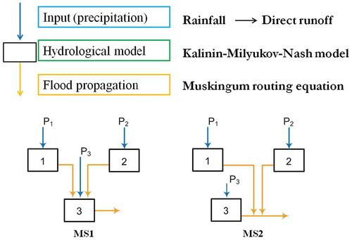
A semi-distributed hydrological model is used to assess the flood hydrograph at the outlet section of the basin and to represent the spatial variability of the uncertain streamflow observations. Two different structures of a semi-distributed Kalinin-Milyukov-Nash model (Szilagyi and Szollosi-Nagy 2010) with Muskingum-type routing are implemented (Fig. 1). In the first model structure (MS1) the sub-basin lumped models are connected in series, so that the hydrograph of an upstream sub-basin is propagated along the successive downstream sub-basins. In the second model structure (MS2), a common structure in many semi-distributed and distributed hydrological models, the sub-basins are connected in parallel. This means that the hydrograph of a sub-basin is directly propagated through the model to the basin outlet where it is aggregated with the outputs of all the other sub-basin models.

Figure 1. Hydrological conceptual model and proposed model structures.

The hydrological modelling framework implemented in each sub-basin, together with the data assimilation approach, is described in Mazzoleni et al. (2015). Evaluation of the direct runoff in each sub-basin is carried out using the Soil Conservation Service curve number (SCS-CN) method. The calibration of the average CN value within the basin is performed by comparing the observed and simulated volume of the quickflow at the outlet section using the SCS-CN method.

The lumped conceptual model used to estimate the quickflow Q is based on the continuous Kalinin-Milyukov-Nash (Szilagyi and Szollosi-Nagy 2010) equation as a convolution of the input, direct runoff I, with the impulse-response function h:

(1)

where n is the number of storage elements in each sub-basin t is time, tau is the integration variable and k is the storage constant. In this study, the parameter k is a linear function between the time of concentration, assessed using the Giandotti equation (Giandotti 1933), and the calibration coefficient c. In order to apply the data assimilation approach, Equation (1) is expressed as a discrete state-space system:

(2)

(3)

where z is the considered sub-basin, x is the model state vector, H is the output matrix and Q is the model discharge value at the time step t. The noises of the system and measurements are represented by the system and observation noises, w_t and v_t, which are normally distributed with zero mean and covariance S and R, respectively. The state-transition and input-transition matrices, Φ and Γ, estimated by Szilagyi and Szollosi-Nagy (2010), are:

(4)

(5)

where Δt is the model time step. Finally, the flow hydrograph of each sub-basin is propagated downstream using the Muskingum channel routing method (Cunge 1969).

2.2 Data assimilation

Data assimilation techniques are used to update model states as a response to real-time observations of significant hydrological variables. In this study, the states of the conceptual model are updated using the well-known and widely used ensemble Kalman filter (EnKF) (Evensen 2003, Mazzoleni et al. 2015). The forecasted probability density distribution (pdf) can be represented by an ensemble of model realizations computed using a Monte Carlo method:

(6)

where x is the forecasted matrix of the model state in the sub-basin z, N is the number of ensemble realizations, and i is an element (realization) of such an ensemble. The model error covariance matrix can be calculated as proposed by Evensen (2003):

(7)

where E is the ensemble anomaly for each ensemble member calculated as:

(8)

where is the ensemble mean of the forecasted state matrix. When an observation becomes available in a sub-basin z at time step t, each member of the perturbed normally distributed measurement vector Q_obs is assimilated with a member of the forecasted matrix of the model state to generate an updated estimate of the model pdf. The update equation is:

(9)

where the Kalman gain K, a weighted factor between model and observations error, is defined as:

(10)

where is the update (or analysis) model state matrix. In the EnKF the efficiency of the filter is closely dependent on the ensemble size (Pauwels and De Lannoy 2009). The ensemble is estimated by perturbing the forcing data and the parameters using a uniform distribution:

(11)

(12)

where I is the forcing value (direct runoff) at the time step t, c is the only perturbed model parameter, ε_I is the fractional input error and ε_p is the fractional parameter error. Based on the results obtained by Mazzoleni et al. (2015), we decided to set n_ens to 65, and ε_I and ε_p equal to 0.2 and 0.9 for MS1, and 0.1 and 0.5 for MS2, respectively.

In this study, the ensemble of synthetic streamflow observations Q_obs, for each single sub-basin z, normally distributed with the mean Q_true and covariance R_t, is generated as:

(13)

where γ is a parameter that accounts for the uncertain (biased) estimation of the discharge observations (see next sections).

2.3 Spatial distribution of sensors within the basin

The correct evaluation of interior streamflow sensor positions is fundamental in properly predicting the flood hydrograph, which may lead to better decisions that reduce flood risk. For this reason, in order to assess the effect of assimilation of distributed streamflow observations within hydrological modelling we followed a general three-step approach (see Fig. 2) applicable for any flood event.

Figure 2. Representation of the three-step method used to assess the effect of sensor location on the DA performance. The NNSE values and locations of sensors shown in steps 2 and 3 are hypothetical.

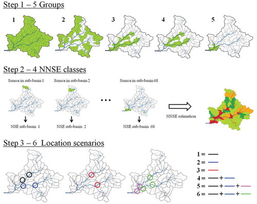
Step 1: A preliminary analysis to assess the performance of the models when assimilating distributed discharge observations from a set of locations in the basin (called “groups”) is carried out. Group 1: in all the sub-basins; Group 2: in the sub-basins with Horton order 1; Group 3: in the main river reach (Horton order 3); Group 4: in the sub-basins on the main channel without those located next to the outlet section; and Group 5: in the sub-basins located close to the outlet cross-section (see Fig. 2).

Step 2: In order to assess the responsiveness of additional measurements in a single location, streamflow observations are assumed to be available at any moment only in a single sub-basin. The model accuracy is evaluated using the Nash-Sutcliffe efficiency (NSE) index, which compares the simulated and the observed discharge hydrographs at the basin outlet. The single NSE values of each sub-basin are then normalized resulting in a normalized NSE (NNSE):

(14)

where Z is the total number of sub-basins. The NNSE is used to compare the results for different flood events since the magnitude of NSE can vary. Therefore, the NNSE are grouped into four classes for different flood events. In this way, the sub-basins that induce a significant improvement in the flood hydrograph are identified for both MS1 and MS2 and a given flood event.

Step 3: Based on the class and the NNSE value of each sub-basin, different scenarios of sensor locations that would give the best model improvement are introduced for the specific flood event. The procedure used in this study to assess such scenarios—applicable to case studies having two main reaches—is schematized as follows:

Scenario 1: Two sensors, in one of the main river branches, located in the sub-basins with the highest class and with the corresponding highest NNSE;

Scenario 2: Two sensors, in the other main river branch, located in the sub-basins with the highest class and with the corresponding highest NNSE;

Scenario 3: Two sensors, in the two opposite river branches, located in the sub-basins with the highest class and with the corresponding highest NNSE;

Scenario 4: Sensors located in the sub-basins considered in scenarios 1 and 2;

Scenario 5: Two additional sensors to those considered in Scenario 4, located in the sub-basins having high class but lower NNSE values than those in Scenario 4, towards the downstream. In this way, it is possible to assess the responsiveness of downstream sub-basins in the streamflow assimilation; and

Scenario 6: Three additional sensors to those considered in Scenario 4, located in random sub-basins having high class but lower NNSE values than those in Scenario 4. This scenario is included in the procedure in order to assess the influence of the total number of sensors.

In the description of the different scenarios, we referred to “in the sub-basin” since we assumed that a measurement taken at the outlet of the sub-basin would provide the same information as an observation at a random location inside the sub-basin. It is worth noting that this procedure does not aim to search exhaustively for all M possible sensor location combinations, or replace traditional optimization methods, but only those related to the classes that show significant model improvement at the outlet section of the basin.

2.4 Sources of uncertainty in the streamflow data quality

In order to represent observation accuracy, different sources of uncertainty that might affect the quality of the observed streamflow data are introduced. As pointed out by Clark et al. (2008), the uncertainty coming from discharge observations can be due to (a) incorrect estimation of water level at a given location, or (b) inaccurate (uncertain) transformation of water level into discharge (rating curve). As reported by Di Baldassarre and Montanari (2009), the uncertainty induced by imperfect measurement of river stage can be negligible when using a static physical sensor. For this reason, in most of the data assimilation applications in hydrology, only the errors caused by an inaccurate rating curve are considered. However, we considered this source of uncertainty in order to assess its effect on the DA procedure. Under these assumptions, Weerts and El Serafy (2006) and Clark et al. (2008) assumed that the error in the streamflow observations should be quantified as a noise term, normally distributed, with zero mean and given covariance:

(15)

where α is a parameter usually assumed to be equal to 0.1 (Weerts and El Serafy 2006, Clark et al. 2008, Rakovec et al. 2012). In order to assess the effect of observation accuracy on DA performance, different sources of uncertainty are considered, assuming a perfect forecast. Figure 3 illustrates various types of observational error, which can be characterised as follows:

• Uncertain rating curve (ErrRC): Uncertainty comes from an inadequate estimation of the rating curve used to transform water level into discharge, whereas the uncertainty induced by imperfect measurements of water level is assumed to be negligible. A normal distribution of the observational error is assumed, with a value of α_RC equal to 0.1, as usually proposed in hydrological data assimilation applications (Weerts and El Serafy 2006, Clark et al. 2008). This type of observational error is used in this study to assess the effect of sensor distribution.

• Uncertain WL estimation (ErrWL): Uncertainty comes from the imperfect measurements of water level, and not from the rating curve estimation. In this case, two different probability distributions, namely normal (WL1) and uniform (WL2), are used to characterize the vector of observations. It is worth noting that EnKF provides optimal results only if the distribution of the measurement vector is Gaussian (however, it can be used with any distribution). For these reasons, the results that are obtained in the WL2 case can be considered as “sub-optimal” with respect to the EnKF assumptions. In addition, due to the fact that errors in the measurements are negligible (Di Baldassarre and Montanari 2009) and smaller than the error in the rating curve estimation, the coefficient α_WL is assumed equal to 0.02.

• Uncertain static sensors (ErrRC+WL). The errors coming from an uncertain rating curve and uncertain WL measurements are considered together. In this case, the value of the coefficient α in Equation (15) is assumed equal to the sum of the two previous coefficients α_RC (ErrRC) and α_WL (ErrWL1), resulting in an observational error normally distributed with zero mean and standard deviation of α·Q_true with α set to 0.12.

• Uncertain estimation of the discharge observation (ErrSD). In this case it is assumed that the value Q_true might be biased and different from the real one. For this reason, the parameter γ (usually set to 1) is considered as a random uniform number between −0.3 and +0.3 in order to account the uncertainty in estimation of Q_true.

Figure 3. Representation of main sources of uncertainty in streamflow measurement.

A graphical representation of the methodology proposed in this study is shown in Figure 4 and Table 1.

Table 1. Summary of simulations as a combination of distribution of sensor locations (groups and scenarios) with different types of observation errors (Err) for the considered flood events. ErrRC: uncertain rating curve; ErrWL: uncertain water-level estimation; ErrRC+WL: uncertain static sensors; ErrSD: uncertain estimation of the discharge observation.

	MS1				MS2
	ErrRC	ErrWL	ErrRC+WL	ErrSD	ErrRC	ErrWL	ErrRC+WL	ErrSD
Group 1	X	–	–	–	X	–	–	–
Group 2	X	–	–	–	X	–	–	–
Group 3	X	X	X	X	X	X	X	X
Group 4	X	X	X	X	X	X	X	X
Group 5	X	X	X	X	X	X	X	X
Scenario 1	X	–	–	–	X	–	–	–
Scenario 2	X	–	–	–	X	–	–	–
Scenario 3	X	–	–	–	X	–	–	–
Scenario 4	X	–	–	–	X	–	–	–
Scenario 5	X	–	–	–	X	–	–	–
Scenario 6	X	X	X	X	X	X	X	X

Figure 4. Values of α and γ according to the different types of source of uncertainty.

3 Case study and model set-up

The case study is located in the Brue basin, in Somerset, southwest UK. It has a drainage area of about 135 km² at Lovington, the basin outlet. The time of concentration, estimated by the equation proposed by Giandotti (1933), is about 10 hours. The streamflow network is derived from the DTM (SRTM dataset with 90 m resolution). The hourly precipitation and streamflow data used in this study are supplied by the British Atmospheric Data Centre from the NERC (Natural Environment Research Council) Hydrological Radar Experiment Dataset. The average precipitation value in each sub-basin is estimated using ordinary kriging, which allows optimal interpolation of point data from the 49 rainfall stations available in the Brue basin (Matheron 1963).

In order to represent the spatial variability of streamflow observations, the Brue basin is divided into 68 sub-basins each having a small drainage area (on average around 2 km²). This makes it possible to assume that any observation assimilated within a given sub-basin provides the same information as an observation at the outlet of same sub-basin, and that in this way distributed streamflow is considered (Mazzoleni et al. 2015). Due to the fact that real streamflow observations are not available in each sub-basin, synthetic values of Q_true are estimated following the approach used in Mazzoleni et al. (2015), i.e. adding a white noise to the time series of input rainfall and model parameter.

The model parameters c and n are calibrated by minimizing the difference (NSE) between the simulated and observed values of discharge at the outlet point of the Brue basin during the flood event that occurred between 16 December 1995 and 1 January 1996. The resulting optimal values of c and n for MS1 and MS2 are found to be c = 1.1, n = 1 and c = 0.8, n = 10, respectively. The basin is relatively small, so these values are assumed to be the same for all sub-basins.

The hydrological model and the EnKF approach are validated by comparing the results obtained for five different flood events that occurred between 28 October and 7 November 1994 (flood event A), between 8 and 16 November 1994 (flood event B), between 4 and 8 January 1994 (flood event C), between 6 and 9 December 1994 (flood event D) and between 31 January and 3 February 1995 (flood event E). The validation analysis shows that flood event A is represented by the semi-distributed hydrological model quite well for both the models, while for other flood events neither model structure provides satisfactory results.

4 Results

4.1 Effect of sensor positioning

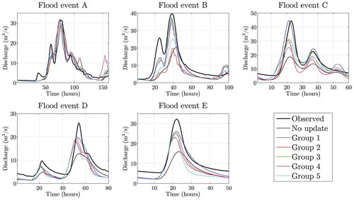
Figures 5 and 6 show the results obtained when assimilating streamflow observations in the location groups described in Section 2.3 during the five considered flood events. It is worth noting that the analyses presented in this section are carried out considering only the uncertainty in rating curve (ErrRC), i.e. α = 0.1. Overall, even with different intensities, assimilation of streamflow observations tends to improve the model results. In particular, MS1 tends to provide greater model improvements than MS2 (e.g. flood events C and D). As expected, assimilation from all the sub-basins (Group 1) provides the best model performances for both MS1 and MS2. In contrast, it can be observed that assimilation from upstream sub-basins (Group 2) does not provide a relevant improvement in the accuracy of the outflow hydrograph. Availability of sensors along the main river channel (Group 3) gives good model results, comparable with the results of Group 1, for both MS1 and MS2. It is interesting to note that, in the case of MS1, assimilation of observations from Group 5 (sensors closed at the basin outlet) results in better model performance than assimilation of observations from Group 4 (sensors located at the upstream part of the main river channel). Opposite results are achieved in the case of MS2. These results are summarized in terms of NSE in Table 2.

Table 2. Results, expressed in terms of NSE, for different spatial distributions of static sensors during the five considered flood events.

	Event A		Event B		Event C		Event D		Event E
	MS1	MS2	MS1	MS2	MS1	MS2	MS1	MS2	MS1	MS2
Group 1	0.93	0.90	0.79	0.87	0.95	0.86	0.73	0.62	0.78	0.85
Group 2	0.90	0.86	0.46	0.38	0.51	0.44	0.56	0.47	0.53	0.58
Group 3	0.93	0.91	0.77	0.81	0.95	0.86	0.73	0.58	0.76	0.76
Group 4	0.92	0.90	0.69	0.82	0.92	0.86	0.72	0.59	0.68	0.75
Group 5	0.93	0.91	0.75	0.64	0.91	0.82	0.72	0.51	0.76	0.65

Figure 5. Comparison between observed hydrograph, model results and data assimilation results considering different sensor locations within main basin groups during all flood events in MS1.

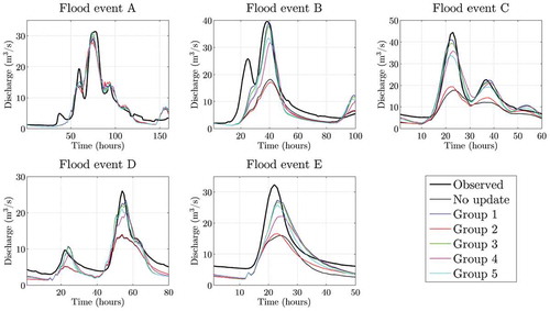
Figure 6. Comparison between observed hydrograph, model results and data assimilation results considering different sensor locations within main basin groups during all flood events in MS2.

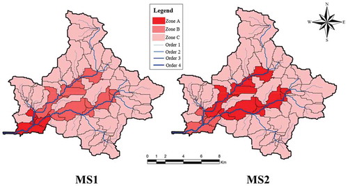
Based on the previous results and considerations, a three-zone map of sensor locations for both model structures is given in Figure 7. Zone C corresponds to observations that do not affect the outflow hydrograph. Overall, observations coming from Zone A lead to the best improvement of model output. In particular, Zone A corresponds to groups 5 and 4 for MS1 and MS2, respectively. Zone B indicates those sub-basins that do provide a noticeable improvement of model results but still lower than that achieved in Zone A.

Figure 7. Indication of the ideal location of the uncertain streamflow observations to assimilate according to the improvements produced by the two proposed model structures.

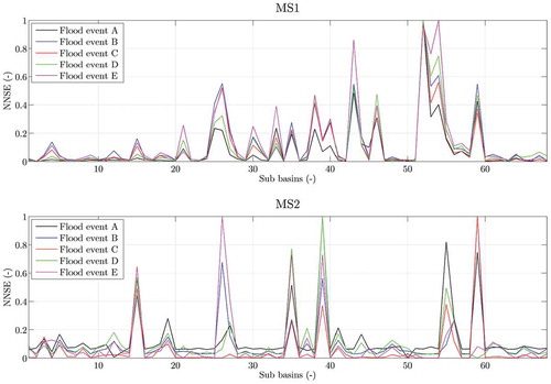
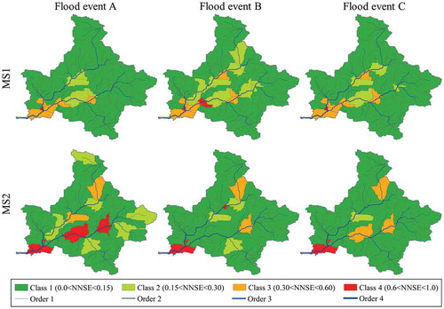
The next step is to assess the model performance considering available streamflow observations in each sub-basin. Figure 8 shows the NNSE values obtained from the assimilation of streamflow observations in a single sub-basin per time for the two model structures during the five flood events. The results show that locations of the sub-basins that provide high NNSE values change from MS1 to MS2. As previously stated, these sub-basins are located mostly along the main river channel (Horton order greater than 3). However, such locations, for a given model structure, are very similar when changing the type of flood event. Overall, MS2 provides lower NNSE values than MS1. In the case of MS2, few sub-basins give high NNSE values, while for MS1 high NNSE values are spread over a larger number of sub-basins.

Figure 8. Indication of the responsiveness of each sub-basin, in terms of NNSE, according to the locations of the uncertain streamflow observations considering the two proposed model structures during the five flood events.

Figure 9 shows the four classes obtained for flood events A, B and C for MS1 and MS2. Similar results are achieved for flood events D and E. As may be seen, analogous locations of the sub-basins having classes 3 and 4 are obtained for the three considered flood events for each structure.

Figure 9. Estimated classes of each sub-basin considering the two proposed model structures during the flood events A, B and C.

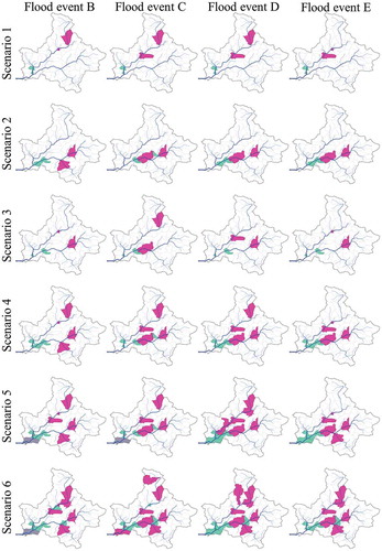
Knowing the NNSE values in each sub-basin, it is possible to assess the six sensor location scenarios for both MS1 and MS2. In Table 3, the total number of sensors used in the different scenarios is reported. Figure 10 shows the locations of sensors for the six different scenarios in four flood events. Overall, sensor location does not vary much for the different flood events. For example, in MS1 and scenarios 3 and 4 the sensors are located in the same sub-basins (represented by light blue) during the four analysed events. Interestingly, in MS1 the sensors are located in the downstream part of the basin, which corresponds to Group 5 or Zone A analysed previously. In MS2, sensors are mainly located in the upstream part of the Brue basin, as previously shown in Zone A of this model structure.

Table 3. Number of sensors according to the six sensor location scenarios within the Brue basin.

Scenario	1	2	3	4	5	6
Number of sensors	2	2	2	4	5	7

Figure 10. Sensor locations in the six scenarios for MS1 (light blue) and MS2 (magenta) during events B, C, D and E. The dark blue areas indicate the same sensor locations for both MS1 and MS2.

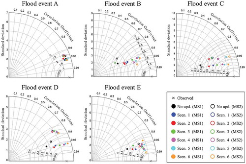
Figure 11 shows the Taylor diagram for the five different events, six scenarios and two model structures. Taylor diagrams graphically summarize similarities between simulations and observations expressed in terms of root mean square error, correlation and standard deviation. The closer the simulation result is to the observations (cross, ×), the better. The simulation results in the case of flood event A are very close to each other due to good model performance without update. As expected, the best model improvement is achieved for a high number of sensors (i.e. Scenario 6) for all the flood events. However, similar improvements can be also observed with scenarios 4 and 5. In the case of flood events B and E, MS2 provides better model results than MS1. However, in the case of flood events C and D, MS1 outperforms MS2. Good correlation values are achieved in all flood events. The low standard deviation values are due to the underestimation of simulated discharge values without model update.

Figure 11. Taylor diagrams comparing observations with simulations obtained with MS1 and MS2 for all flood events and different sensor location scenarios.

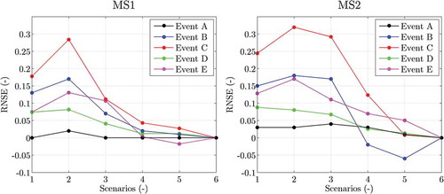
Figure 12 shows the relative NSE (RNSE) expressed as the difference between the NSE values of each given scenario and that of Scenario 6, i.e. the one that provides the best model results, during the five flood events. Overall, in both structures, high RNSE values are achieved with scenarios 1, 2 and 3. Such values decrease for scenarios 4 and 5. The main difference between MS1 and MS2 is that, on average, the RNSE values of Scenario 4 are higher in MS2 than MS1. This means that MS2 is more sensitive to the total number of sensors than MS1. Low RNSE improvements are shown in the case of flood event A due to the already high NSE value without model updates.

Figure 12. Relative NSE between sensor location scenarios 1, 2, 3 4 and 5 compared with Scenario 6 for MS1 and MS2 and all flood events.

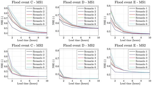
Figure 13 shows the relation between NSE and lead-time values for MS1 and MS2 during flood events C, D and E. It can be observed that MS2 tends to the NSE values without model update faster (after 4 h) than MS1. In all flood events, Scenario 6 provides the best model performances. It can also be seen that Scenario 4 gives similar model results to Scenario 6 in MS1 for different lead times, as previously demonstrated. Lowest performances are obtained with scenarios 1, 2 and 3.

Figure 13. NSE obtained for different values of lead time in the assimilation of streamflow observations for the six sensor location scenarios and flood events C, D and E.

4.2 Effect of observation accuracy

In this analysis, the effects of different observation accuracies on model performance are assessed. Firstly, we consider the assimilation of streamflow observation within the main Brue basin groups in the case of only MS1, and then within Scenario 6 for both MS1 and MS2 during the flood events C, D and E.

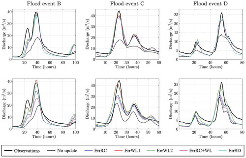
From Figure 14 it can be seen that the best model improvement is achieved by assuming only the error coming from the measurements, i.e. ErrWL1 with normal or ErrWL2 with uniform distribution, in all the considered flood events for sensors located in the sub-basins of Group 3. It can be seen that better results are obtained for uncertain biased streamflow values (ErrSD) compared to considering only ErrRC. Overall, the smallest model improvements are achieved when considering ErrRC+WL. An important result is that MS2 seems to be more sensitive to the proper definition of observational error than MS1.

Figure 14. Outflow hydrographs obtained for four Group 3 spatial sensor locations in the case of MS1 (upper row) and MS2 (lower row) considering different types of observational error in the DA procedure.

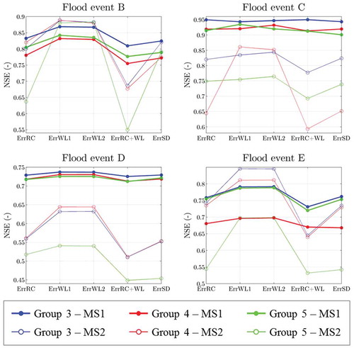
Figure 15 shows the NSE values for MS1 and MS2 for the definition of different observational errors during events B, C, D and E. Sensors are assumed to be located in groups 3, 4 and 5. For events C and D, MS1 gives higher NSE values than MS2. As previously demonstrated, the variability of NSE values is higher in MS2 than MS1 for different observational errors. In addition, small differences between the NSE values are obtained with ErrWL1 and ErrWL2.

Figure 15. NSE for different observational errors obtained for flood events B, C, D and E considering sensors located in groups 3, 4 and 5.

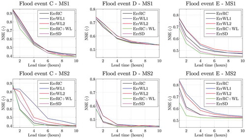
Figure 16 shows the prediction of flood events C, D and E with sensors located according to Scenario 6 for MS1 and MS2. The results obtained for shorter lead times are in agreement with those shown in Figure 15 for different sensor locations. Overall, MS1 seems to be less sensitive to the observational errors compared to MS2, also for long lead times. However, large variability of NSE is obtained during flood event E using MS1. The best predictive efficiency is obtained for both model structures in the case of ErrWL, as previously described in Figures 14 and 15, with a lead time of 1 h. On average, ErrRC+WL provides the lowest NSE values. Small differences between NSE obtained for ErrRC and ErrSD are shown for both MS1 and MS2. Moreover, the difference between ErrRC and ErrRC+WL is greater for MS2 than for MS1 for low lead time. It is interesting to observe that NSE values simulated with ErrWL for flood event C and MS2 are lower than those obtained with the other observational errors for 1 h lead time. However, for longer lead times, ErrWL1 and ErrWL2 give the best model improvements. The difference between NSE obtained using different observational errors tends to be negligible in both MS1 and MS2 for long lead times. In particular, for lead times comparable with the time of concentration of the basin, the NSE values obtained with the different observational errors tend to the one achieved without model update.

Figure 16. Relationship between NSE and different lead times for diverse types of observational error during flood events C, D and E considering Scenario 6 for both MS1 and MS2.

5 Discussion

Assimilation of distributed streamflow observations was performed in the Brue catchment for five flood events considering two different structures of a semi-distributed hydrological model.

In general, assimilation of discharge measurements located in a river channel with Horton order equal to or greater than 3 tends to better represent the outflow discharge. For all the flood events, model structure MS2 was influenced by both the total number of sensors and their locations (Group 4). In contrast, MS1 was not affected by the total number of sensors, but only by their locations (Group 5). Based on these results, a three-zone map of sensor locations for the Brue basin is proposed. In Zone A are those sub-basins that contribute to generating high model results, while sub-basins in Zone C do not affect model performance. In particular, for MS1, Zone A corresponds to the sub-basins of Group 5, located in the downstream area, which is very often an urbanized area for which timely flood warnings could be especially important. The observations of discharge from this zone might indeed improve the model results in terms of outflow, but at the same time they do not provide enough time to react in the downstream areas where floods could be very damaging. However, assimilation of observations from Zone B (Group 4) might induce an insubstantial improvement in model accuracy if compared to Group 5, but it would give enough warning time before the estimated (high) flow reaches the downstream.

The patterns of NNSE values obtained for MS1 and MS2, similar for different flood events, indicate low sensitivity of the model structures to sensor location during these events. This is reflected in similar sensor locations for the six proposed scenarios for both MS1 and MS2. However, from Figure 10, it can be seen that sensor locations vary more for MS2 than MS1 in Scenario 6. As expected, a high number of sensors (Scenario 6) gives the highest NSE values for both MS1 and MS2. However, the difference between model results obtained with scenarios 4 and 6 with MS1 is smaller than that for MS2. This leads to the conclusion that, as already stated, MS1 is more sensitive than is MS2 to the specific location of sensors (Scenario 4) than to their total number (Scenario 6) (see Figs. 11 and 12).

In general, for long lead times, MS1 outperforms MS2. Considering MS1, Scenario 4 provides the best compromise between NSE and number of sensors (four) for lead times shorter than the time of concentration of the basin. However, as shown in Figure 13, there is a significant difference between NSE values obtained in scenarios 4 and 6 with MS2. Model results tend to those obtained without updating for lead times similar to the time of concentration of the basin (10 h).

The analyses carried out for different observational errors demonstrated that less uncertainty in the water depth estimation (ErrWL) produces greater improvements in model performance for both low and high lead times. It is interesting to note that, in both results coming from the probability distributions WL1 and WL2, a similar trend in the outflow hydrographs can be observed (see Figs. 14 and 15). These considerations lead to the conclusion that the “non-optimal” results provided by the EnKF in the case of a uniform distribution are comparable to the optimal solution for 1 h lead time. In problems of assimilation of distributed streamflow observations, using a semi-distributed hydrological model, the uncertainty in rating curve estimation (ErrRC), as expected, has more influence than uncertainty of incorrect estimation of water level made by physical sensors. It can be seen that similar results are obtained for uncertain rating curve estimation and uncertain biased streamflow values (ErrSD). This may be due to the fact that the biased value of Q_true might be compensated because of the semi-distributed nature of the hydrological model. As expected, the lowest model results are obtained in the case of errors in both water depth and rating curve estimation (ErrRC+WL). Finally, MS2 is more sensitive to the proper definition of the observational error than MS1 for both low and high lead times.

6 Conclusions

The main goals of this study were to evaluate the effects of different sensor locations and observation accuracy on the assimilation of distributed streamflow observations in hydrological modelling, with the aim of improving flood forecasting. Two different model structures (MS) of a semi-distributed hydrological model were considered. In order to assimilate streamflow observations, an ensemble Kalman filter was implemented in each model structure.

From the results of this study it can be concluded that the assimilation of distributed observations in the main river channel induces the best model improvement for both model structures. Overall, flood prediction with MS2 was influenced by the total number of sensors and by their locations, while that with MS1 was only affected by the sensor locations and not by the total number of sensors. One of the main conclusions is that the sensor locations which generate highest NSE and NNSE values at the basin outlet do not significantly change according to the given flood event and model structure. However, when only MS2 was considered, it was demonstrated that the locations of a high number of sensors (more than four) changed according to the given flood event. Therefore, designing flow sensor networks considering a longer time series of flood events might be inappropriate since the effect of the single flood event is diminished. For this reason, additional efforts towards the development of techniques to design networks of dynamic low-cost sensors should be carried out. In the case of flood prediction, MS1 tends to outperform MS2 for high lead-time values. It is worth noting that the results we obtained are valid only in the considered case study and for five different flood events

This study indicates the importance of the proper definition of observation accuracy in DA performance. In fact, considering only the accuracy in the water-level measurements (ErrWL) has significant effects on the improvement of outflow hydrograph prediction—if compared to the results obtained when error in biased streamflow observations (ErrSD) and rating curve uncertainty (ErrRC) are considered. Both MS1 and MS2 are influenced by the different types of observation accuracy only for short lead times, while for long lead times NSE tends to be similar in all the assumed observation errors. However, MS2 is more sensitive than MS1 to different types of observation accuracy for short lead times.

It is important to mention certain limitations of this study. Firstly, only five flood events were considered, so additional experiments are recommended to generalize the conclusions in different case studies. In fact, the results should be considered valid only for basins with characteristics similar to those of the Brue basin. Moreover, the value of the coefficient α of Equation (15), in the case of ErrRC+WL, is assumed equal to the sum of the two previous coefficients α_RC and α_WL. Additional studies should be carried out to consider the combined error in both measurements and to use a joint probability distribution to characterize the rating curve uncertainty.

For future studies it is also recommended to (a) carry out a more detailed analysis using a higher number of events to further validate the results, (b) employ other types of hydrological models to explore how the internal model structure affects the filter performance, and (c) pose and solve a fully-fledged optimization problem aimed at identifying the best sensor topology for typical flood forecasting problems. A specific challenge is of course introducing the proposed methodology in real management practice.

Acknowledgements

Data used were supplied by the British Atmospheric Data Centre from the NERC Hydrological Radar Experiment Dataset http://www.badc.rl.ac.uk/data/hyrex/. The Associate Editor Professor Giuliano Di Baldassarre and two anonymous reviewers are also acknowledged for their valuable comments.

Disclosure statement

No potential conflict of interest was reported by the authors.

Additional information

Funding

This research is funded in the framework of the European FP7 Project WeSenseIt: Citizen Observatory of Water [grant agreement no. 308429].

References

- Alfonso, L., Lobbrecht, A., and Price, R., 2010. Optimization of water level monitoring network in polder systems using information theory. Water Resources Research, 46 (12), W12553. doi:10.1029/2009WR008953
- Alfonso, L. and Price, R., 2012. Coupling hydrodynamic models and value of information for designing stage monitoring networks. Water Resources Research, 48 (8), W08530. doi:10.1029/2012WR012040
- Andreadis, K.M. and Lettenmaier, D.P., 2006. Assimilating remotely sensed snow observations into a macroscale hydrology model. Advances in Water Resources, 29 (6), 872–886. doi:10.1016/j.advwatres.2005.08.004
- Arulampalam, M.S., et al., 2002. A tutorial on particle filters for online nonlinear/non-Gaussian Bayesian tracking. IEEE Transactions on Signal Processing, 50 (2), 174–188. doi:10.1109/78.978374
- Aubert, D., Loumagne, C., and Oudin, L., 2003. Sequential assimilation of soil moisture and streamflow data in a conceptual rainfall–runoff model. Journal of Hydrology, 280 (1–4), 145–161. doi:10.1016/S0022-1694(03)00229-4
- Bárdossy, A. and Das, T., 2008. Influence of rainfall observation network on model calibration and application. Hydrology and Earth System Sciences Discussions, 12 (1), 77–89. doi:10.5194/hess-12-77-2008
- Beven, K.J., 2004. Rainfall - runoff modelling: the primer. Chichester, UK: John Wiley & Sons.
- Blöschl, G., Reszler, C., and Komma, J., 2008. A spatially distributed flash flood forecasting model. Environmental Modelling & Software, 23 (4), 464–478. doi:10.1016/j.envsoft.2007.06.010
- Brocca, L., et al., 2010. Improving runoff prediction through the assimilation of the ASCAT soil moisture product. Hydrology and Earth System Sciences, 14 (10), 1881–1893. doi:10.5194/hess-14-1881-2010
- Brocca, L., et al., 2012. Assimilation of surface- and root-zone ASCAT soil moisture products into rainfall–runoff modeling. IEEE Transactions on Geoscience and Remote Sensing, 50 (7), 2542–2555. doi:10.1109/TGRS.2011.2177468
- Cañizares, T.R., 1999. On the application of data assimilation in regional coastal models. Rotterdam: Balkema.
- Chen, J., et al., 2012. Assimilating multi-site measurements for semi-distributed hydrological model updating. Quaternary International, 282, 122–129. doi:10.1016/j.quaint.2012.01.030
- Clark, M.P., et al., 2008. Hydrological data assimilation with the ensemble Kalman filter: use of streamflow observations to update states in a distributed hydrological model. Advances in Water Resources, 31 (10), 1309–1324. doi:10.1016/j.advwatres.2008.06.005
- Cunge, J.A., 1969. On the subject of a flood propagation computation method (Muskingum Method). Journal of Hydraulic Research, 7 (2), 205–230. doi:10.1080/00221686909500264
- Di Baldassarre, G. and Montanari, A., 2009. Uncertainty in river discharge observations: a quantitative analysis. Hydrology and Earth System Sciences Discussions, 6 (1), 39–61. doi:10.5194/hessd-6-39-2009
- Evensen, G., 2003. The ensemble Kalman filter: theoretical formulation and practical implementation. Ocean Dynamics, 53 (4), 343–367. doi:10.1007/s10236-003-0036-9
- Fischer, C., et al., 2005. An overview of the variational assimilation in the ALADIN/France numerical weather-prediction system. Quarterly Journal of the Royal Meteorological Society, 131 (613), 3477–3492. doi:10.1256/qj.05.115
- Fowler, A. and Jan Van Leeuwen, P., 2013. Observation impact in data assimilation: the effect of non-Gaussian observation error. Tellus A, 65. doi:10.3402/tellusa.v65i0.20035
- Giandotti, M., 1933. Previsione delle piene e delle magre dei corsi d’acqua. Rome: Servizio Idrografico Italiano.
- Giustarini, L., et al., 2011. Assimilating SAR-derived water level data into a hydraulic model: a case study. Hydrology and Earth System Sciences, 15 (7), 2349–2365. doi:10.5194/hess-15-2349-2011
- Houser, P.R., et al., 1998. Integration of soil moisture remote sensing and hydrologic modeling using data assimilation. Water Resources Research, 34 (12), 3405–3420. doi:10.1029/1998WR900001
- Kalman, R.E., 1960. A new approach to linear filtering and prediction problems. Journal of Basic Engineering, 82 (1), 35–45. doi:10.1115/1.3662552
- Kavetski, D., Kuczera, G., and Franks, S.W., 2006. Bayesian analysis of input uncertainty in hydrological modeling: 1. Theory. Water Resources Research, 42 (3), W03407.
- Kollat, J.B., Reed, P.M., and Maxwell, R.M., 2011. Many-objective groundwater monitoring network design using bias-aware ensemble Kalman filtering, evolutionary optimization, and visual analytics. Water Resources Research, 47 (2), W02529. doi:10.1029/2010WR009194
- Komma, J., Blöschl, G., and Reszler, C., 2008. Soil moisture updating by ensemble Kalman filtering in real-time flood forecasting. Journal of Hydrology, 357 (3–4), 228–242. doi:10.1016/j.jhydrol.2008.05.020
- Lee, H., Seo, D.J., and Koren, V., 2011. Assimilation of streamflow and in situ soil moisture data into operational distributed hydrologic models: effects of uncertainties in the data and initial model soil moisture states. Advances in Water Resources, 34 (12), 1597–1615. doi:10.1016/j.advwatres.2011.08.012
- Lee, H., et al., 2012. Variational assimilation of streamflow into operational distributed hydrologic models: effect of spatiotemporal scale of adjustment. Hydrology and Earth System Sciences, 16 (7), 2233–2251. doi:10.5194/hess-16-2233-2012
- Li, Z. and Navon, I.M., 2001. Optimality of variational data assimilation and its relationship with the Kalman filter and smoother. Quarterly Journal of the Royal Meteorological Society, 127 (572), 661–683. doi:10.1002/(ISSN)1477-870X
- Liu, Y. and Gupta, H.V., 2007. Uncertainty in hydrologic modeling: toward an integrated data assimilation framework. Water Resources Research, 43 (7), 1–18. doi:10.1029/2006WR005756
- Liu, Y., et al., 2012. Advancing data assimilation in operational hydrologic forecasting: progresses, challenges, and emerging opportunities. Hydrology and Earth System Sciences, 16 (10), 3863–3887. doi:10.5194/hess-16-3863-2012
- Lorenc, A.C. and Rawlins, F., 2005. Why does 4D-Var beat 3D-Var? Quarterly Journal of the Royal Meteorological Society, 131 (613), 3247–3257. doi:10.1256/qj.05.85
- Madsen, H. and Cañizares, R., 1999. Comparison of extended and ensemble Kalman filters for data assimilation in coastal area modelling. International Journal for Numerical Methods in Fluids, 31 (6), 961–981. doi:10.1002/(ISSN)1097-0363
- Madsen, H. and Skotner, C., 2005. Adaptive state updating in real-time river flow forecasting - a combined filtering and error forecasting procedure. Journal of Hydrology, 308 (1–4), 302–312. doi:10.1016/j.jhydrol.2004.10.030
- Matheron, G., 1963. Principles of geostatistics. Economic Geology, 58 (8), 1246–1266. doi:10.2113/gsecongeo.58.8.1246
- Mazzoleni, M., et al., 2015. Assimilating uncertain, dynamic and intermittent streamflow observations in hydrological models. Advances in Water Resources, 83, 323–339. doi:10.1016/j.advwatres.2015.07.004
- McLaughlin, D., 1995. Recent developments in hydrologic data assimilation. Reviews of Geophysics, 33 (95), 977–984. doi:10.1029/95RG00740
- McLaughlin, D., 2002. An integrated approach to hydrologic data assimilation: interpolation, smoothing, and filtering. Advances in Water Resources, 25 (8–12), 1275–1286. doi:10.1016/S0309-1708(02)00055-6
- McMillan, H.K., et al., 2013. Operational hydrological data assimilation with the recursive ensemble Kalman filter. Hydrology and Earth System Sciences, 17 (1), 21–38. doi:10.5194/hess-17-21-2013
- McMillan, H.K., et al., 2011. Rainfall uncertainty in hydrological modelling: an evaluation of multiplicative error models. Journal of Hydrology, 400 (1–2), 83–94. doi:10.1016/j.jhydrol.2011.01.026
- Mendoza, P.A., McPhee, J., and Vargas, X., 2012. Uncertainty in flood forecasting: a distributed modeling approach in a sparse data catchment. Water Resources Research, 48 (9). doi:10.1029/2011WR011089
- Moradkhani, H., et al., 2005. Uncertainty assessment of hydrologic model states and parameters: sequential data assimilation using the particle filter. Water Resources Research, 41 (5), W05012. doi:10.1029/2004WR003604
- Moulin, L., Gaume, E., and Obled, C., 2009. Uncertainties on mean areal precipitation: assessment and impact on streamflow simulations. Hydrology and Earth System Sciences, 13 (2), 99–114. doi:10.5194/hess-13-99-2009
- Neal, J.C., Atkinson, P.M., and Hutton, C.W., 2007. Flood inundation model updating using an ensemble Kalman filter and spatially distributed measurements. Journal of Hydrology, 336 (3–4), 401–415. doi:10.1016/j.jhydrol.2007.01.012
- Noh, S.J., et al., 2014. On noise specification in data assimilation schemes for improved flood forecasting using distributed hydrological models. Journal of Hydrology, 519 (Part D), 2707–2721. doi:10.1016/j.jhydrol.2014.07.049
- Pappenberger, F., et al., 2006. Influence of uncertain boundary conditions and model structure on flood inundation predictions. Advances in Water Resources, 29 (10), 1430–1449. doi:10.1016/j.advwatres.2005.11.012
- Pauwels, V.R.N. and De Lannoy, G.J.M., 2006. Improvement of modeled soil wetness conditions and turbulent fluxes through the assimilation of observed discharge. Journal of Hydrometeorology, 7 (3), 458–477. doi:10.1175/JHM490.1
- Pauwels, V.R.N. and De Lannoy, G.J.M., 2009. Ensemble-based assimilation of discharge into rainfall-runoff models: a comparison of approaches to mapping observational information to state space. Water Resources Research, 45 (8), W08428. doi:10.1029/2008WR007590
- Rakovec, O., et al., 2012. State updating of a distributed hydrological model with ensemble Kalman filtering: effects of updating frequency and observation network density on forecast accuracy. Hydrology and Earth System Sciences, 16 (9), 3435–3449. doi:10.5194/hess-16-3435-2012
- Reichle, R.H., 2000. Variational assimilation of remote sensing data for land surface hydrologic applications. Thesis. Massachusetts Institute of Technology.
- Salamon, P. and Feyen, L., 2009. Assessing parameter, precipitation, and predictive uncertainty in a distributed hydrological model using sequential data assimilation with the particle filter. Journal of Hydrology, 376 (3–4), 428–442. doi:10.1016/j.jhydrol.2009.07.051
- Seo, D.J., Koren, V., and Cajina, N., 2003. Real-time variational assimilation of hydrologic and hydrometeorological data into operational hydrologic forecasting. Journal of Hydrometeorology, 4 (3), 627–641. doi:10.1175/1525-7541(2003)004<0627:RVAOHA>2.0.CO;2
- Seo, D.J., et al., 2009. Automatic state updating for operational streamflow forecasting via variational data assimilation. Journal of Hydrology, 367 (3–4), 255–275. doi:10.1016/j.jhydrol.2009.01.019
- Szilagyi, J. and Szollosi-Nagy, A., 2010. Recursive streamflow forecasting: a state space approach. Leiden: CRC Press.
- Todini, E., et al., 2005. ACTIF best practice paper - understanding and reducing uncertainty in flood forecasting. Proceeding of ACTIF Conference, (1), 1–43.
- Valstar, J.R., et al., 2004. A representer-based inverse method for groundwater flow and transport applications. Water Resources Research, 40 (5), W05116. doi:10.1029/2003WR002922
- Verlaan, M., 1998. Efficient Kalman Filtering Algorithms for hydrodynamic models. PhD Thesis. Delft University of Technology, The Netherlands.
- Verlaan, M. and Heemink, A.W., 1996. Data assimilation schemes for non-linear shallow water flow models, Adv. Fluid Mechanics: 96 (1996), pp. 277–286.
- Walker, J.P., Willgoose, G.R., and Kalma, J.D., 2001. One-dimensional soil moisture profile retrieval by assimilation of near-surface observations: a comparison of retrieval algorithms. Advances in Water Resources, 24 (6), 631–650. doi:10.1016/S0309-1708(00)00043-9
- Weerts, A.H. and El Serafy, G.Y.H., 2006. Particle filtering and ensemble Kalman filtering for state updating with hydrological conceptual rainfall-runoff models. Water Resources Research, 42 (9), 1–17. doi:10.1029/2005WR004093
- Xie, X. and Zhang, D., 2010. Data assimilation for distributed hydrological catchment modeling via ensemble Kalman filter. Advances in Water Resources, 33 (6), 678–690. doi:10.1016/j.advwatres.2010.03.012